Article

GPIO-Based Nonlinear Predictive Control for Flux-Weakening Current Control of the IPMSM Servo System

School of Automation, Southeast University, Key Laboratory of Measurement and Control of CSE, Ministry of Education, Nanjing 210096, China
*
Author to whom correspondence should be addressed.
Energies 2020, 13(7), 1716; https://doi.org/10.3390/en13071716
Submission received: 1 March 2020 / Revised: 24 March 2020 / Accepted: 30 March 2020 / Published: 4 April 2020

Abstract

:
This paper proposes a generalized proportional integral observer (GPIO) based nonlinear predictive control (NPC) for an interior permanent magnet synchronous motor (IPMSM) to improve the flux-weakening (FW) current control performance against the complex nonlinear cross-coupling terms and the IPMSM parameters’ variations. First, the IPMSM is remodeled to further analyze the FW control difficulties caused by such cross-coupling terms and parameters variations. Considering the parameters’ variations as a kind of disturbance, a GPIO is then designed to compensate for such disturbance. A GPIO-based NPC is finally designed to handle the nonlinear cross-coupling terms to obtain an optimized current control performance. Experiments on a digital signal processor (DSP) based IPMSM servo system validate the workability of the proposed control scheme.

Graphical Abstract

1. Introduction

The interior permanent magnet synchronous motor (IPMSM) has drawn great attention in the applications of industrial robots, electric vehicles, etc., due to its high performance of a wider speed range and a greater mechanical torque as compared with the surface permanent magnet synchronous motors (SPMSM) [1,2,3]. IPMSM and SPMSM have different permanent magnets’ installation positions in the iron core, and therefore they have different inductance characteristics, i.e., the IPMSM has a bigger quadrature-axis inductance than the direct-axis inductance while the SPMSM has almost the same direct-axis and quadrature-axis inductances. Hence, the IPMSM can provide a considerable reluctance torque (which is a part of the mechanical torque) while the SPMSM has almost no reluctance torque [4,5,6]. Moreover, to exploit the potential performance of IPMSM, a flux-weakening (FW) control framework rather than a traditional i d = 0 control framework must be employed [7,8,9]. The i d = 0 control framework is designed that, for the IPMSM, the reference direct-axis current is given as 0 for simple, and the FW control framework is designed that a minus reference direct-axis current trajectory (to be designed) is given to the IPMSM. There are two great advantages by employing the FW control framework. First, the minus direct-axis current can decrease the stator voltage especially when it is close to the maximum voltage that the inverter can provide, in order to increase the speed of IPMSM to exceed the original maximum speed. Second, a well-designed minus direct-axis reference current can make the IPMSM output a considerable reluctance torque [10,11,12]. Although the flux-weakening control framework has such superiority, it also faces more difficulties in the current controller design. First, note that there are complex nonlinear cross-coupling voltages in the current dynamics of the IPMSM (see Equation (2) for details). Such nonlinear cross-coupling terms become very larger in the FW control framework than those in the i d = 0 control framework [13,14,15,16]. In addition, in fact, the relative small nonlinear cross-coupling terms can simplify the current control design, and this is the main advantage of the i d = 0 control. Second, the FW framework means that the IPMSM is working in a special condition where the speed and current of the motor are much higher than those in the i d = 0 framework. The higher speed and current amplify the effect of motor parameters’ variations (see Equation (5) for details). Hence, to take advantage of the FW control, the current controller must be well-designed to deal with such nonlinear cross-coupling terms and parameters variations [17,18,19,20]. Various closed-loop control strategies are proposed to improve the performance of the FW control of the IPMSM. Reference [21] designs a feedback linearization based control for the FW current control. The performance is good when the motor parameters are accurate. However, since the feedback linearization depends on accurate motor parameters, the performance is not satisfactory in the face of the parameters variations. Reference [22] designs an artificial-neural-network-based control for the FW control. The control performance against the nonlinear cross-coupling terms is further improved, but the neural-network-based control needs very heavy online computation. Reference [23] proposes a linearization-based model predictive control (MPC) for the FW control. The control performance is improved since the nonlinear cross-coupling terms are well handled. However, the motor parameters variations are not considered when designing the MPC, so the robustness needs to be further improved.
In this study, a generalized proportional integral observer (GPIO) based nonlinear predictive control (NPC) is proposed to improve the flux-weakening current control performance against the complex nonlinear cross-coupling terms and the IPMSM parameters variations. The GPIO is first introduced in Reference [24], and it is further investigated and proved to be an effective method to estimate different sources of disturbances [25,26]. In this paper, the parameters’ variations of the IPMSM are treated as a kind of disturbance, and the GPIO is specially designed to suppress such disturbance. Nonlinear predictive control (NPC) is a kind of MPC, and it can solve an optimized control for a nonlinear control system. The NPC is proved to be a superior solution for nonlinear problems [27,28,29,30,31]. In this paper, the basic NPC strategy is employed to handle the nonlinear cross-coupling terms for a satisfactory closed-loop performance. Combining the GPIO to compensate the disturbance caused by parameters variations, the NPC is redesigned to make up the robustness against the disturbance.
The major contributions of this paper include three aspects: (1) The nonlinear cross-coupling terms and the motor parameters’ variations of the IPMSM are remodeled, and then the FW control difficulties caused by them are analyzed in detail. (2) Considering the parameters variations as a kind of disturbance, a GPIO based compensation is designed to suppress such disturbance. The robustness against the parameters variations is guaranteed. (3) On the basis of disturbance compensation, a GPIO-based NPC is designed to handle the nonlinear cross-coupling terms for an optimized closed-loop performance.
Finally, experiments under current and speed control modes are respectively conducted on a DSP-based IPMSM servo system to validate the feasibility and effectiveness of the proposed control scheme. The experimental results have shown that the proposed control scheme can achieve a satisfactory control performance against the nonlinear cross-coupling terms and the parameters variations, as compared with an integral NPC scheme and an improved PI control scheme.

2. Preliminaries

2.1. Current Dynamic Model of IPMSM

Assume that the magnetic circuit is unsaturated, the eddy current and hysteresis loss are ignored, and the three-phase stator windings of IPMSM are sinusoidally distributed in space. Taking the rotor coordinates (d- and q-axes) of the motor as reference coordinates and ignoring the dead-time effects, the voltage equations of the IPMSM can be written in the following forms [4]:
d i d d t = 1 L d 0 ( R s 0 i d + u d + u d c o u p l i n g ) , d i q d t = 1 L q 0 ( R s 0 i q + u q + u q c o u p l i n g ) ,
where R s 0 is the nominal value of the stator resistance, L d 0 and L q 0 are respectively the nominal values of the d- and q-axes stator inductances, i d and i q are respectively the d- and q-axes stator currents, u d and u q are respectively the d- and q-axes stator voltages, and u d c o u p l i n g and u q c o u p l i n g are respectively the d- and q-axes cross-coupling terms. The cross-coupling terms are given by
u d c o u p l i n g = n p ω L q i q , u q c o u p l i n g = n p ω L d i d n p ω ψ f ,
where n p is the number of pole pairs, ψ f is the rotor flux linkage, and ω is the rotor angular speed.
Remark 1.
Nonlinear cross-coupling terms. In Equation (2), the d-axis coupling term n p ω L q i q is related to the q-axis stator current i q , and the q-axis coupling term n p ω L d i d n p ω ψ f is related to the d-axis stator current i d , so they are together called cross-coupling terms. Those multiply-form nonlinear cross-coupling terms grow greater from the constant torque (CT) region to the FW region, so they need major consideration in the current controller design.
Furthermore, considering the motor parameters’ variations, each motor parameter can be expressed as the sum of its nominal value and change, given by
R s = R s 0 + Δ R s , L d = L d 0 + Δ L d , L q = L q 0 + Δ L q , ψ f = ψ f 0 + Δ ψ f ,
where R s 0 and Δ R s are respectively the nominal value and change of stator resistance, L d 0 and Δ L d are respectively the nominal value and change of d-axis stator inductance, L q 0 and Δ L q are respectively the nominal value and change of q-axis stator inductance, and ψ f 0 and Δ ψ f are respectively the nominal value and change of rotor flux linkage. Substituting Equation (3) into Equation (1), the dynamic model of the IPMSM from Equation (1) can be rewritten as
d i d d t = 1 L d 0 ( u d R s 0 i d + n p ω L q 0 i q + p d ) , d i q d t = 1 L q 0 ( u q R s 0 i q n p ω L d 0 i d n p ω ψ f 0 + p q ) ,
where p d and p d are respectively the d- and q-axes time-varying voltages terms, given by
p d = Δ R s i d + n p ω Δ L q i q Δ L d d i d d t , p q = Δ R s i q n p ω Δ L d i d n p ω Δ ψ f Δ L q d i q d t .
Remark 2.
Motor parameters’ variations. The terms p d and p d caused by the motor parameters’ variations are time-varying, and moreover they grow greater from the CT region to the FW region. Hence, they also need major consideration in the current controller design.

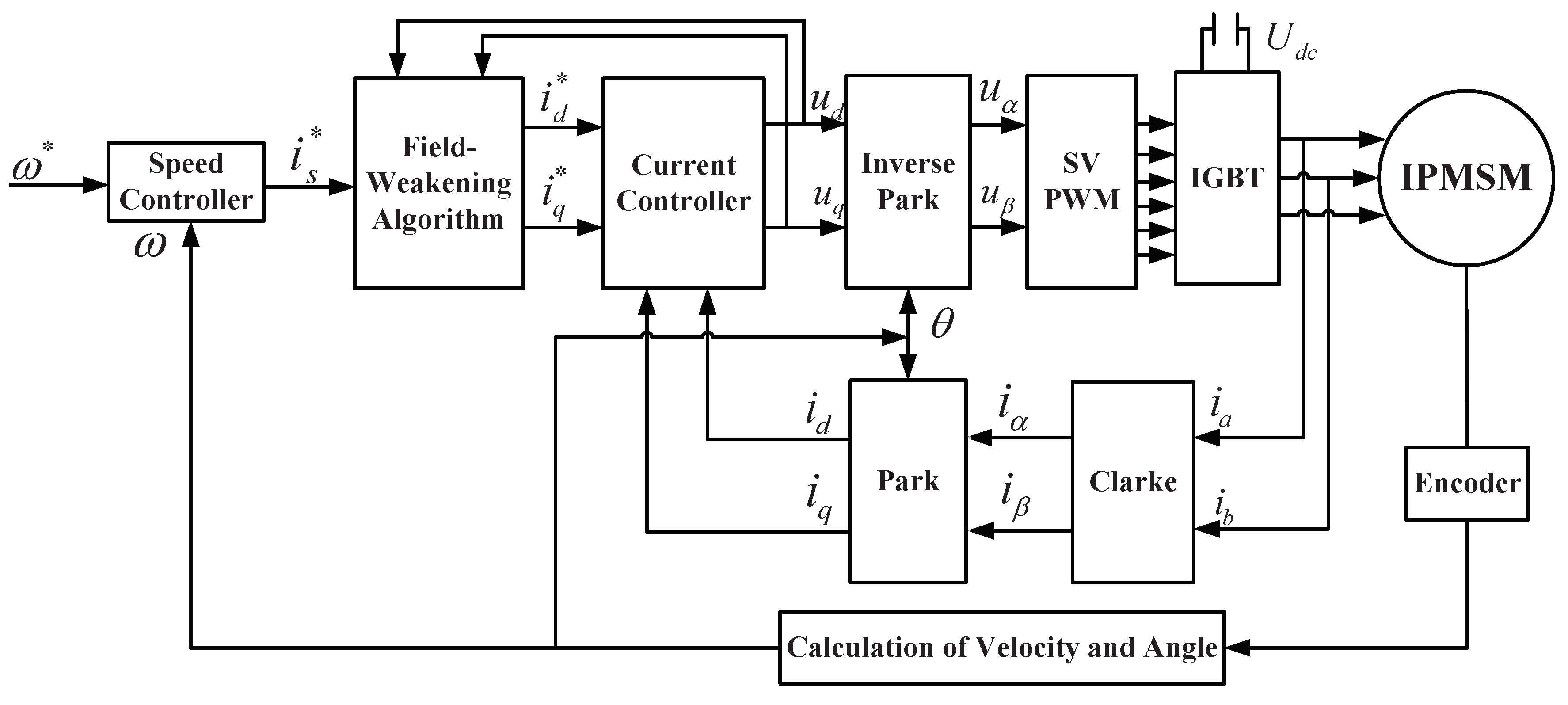
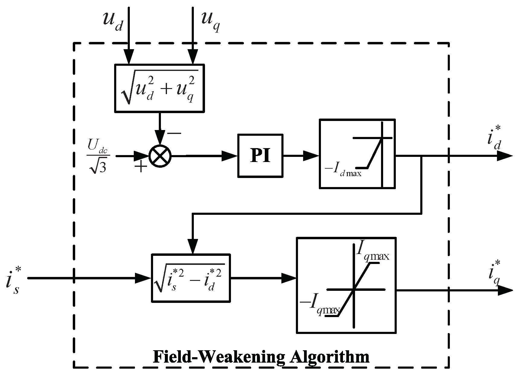
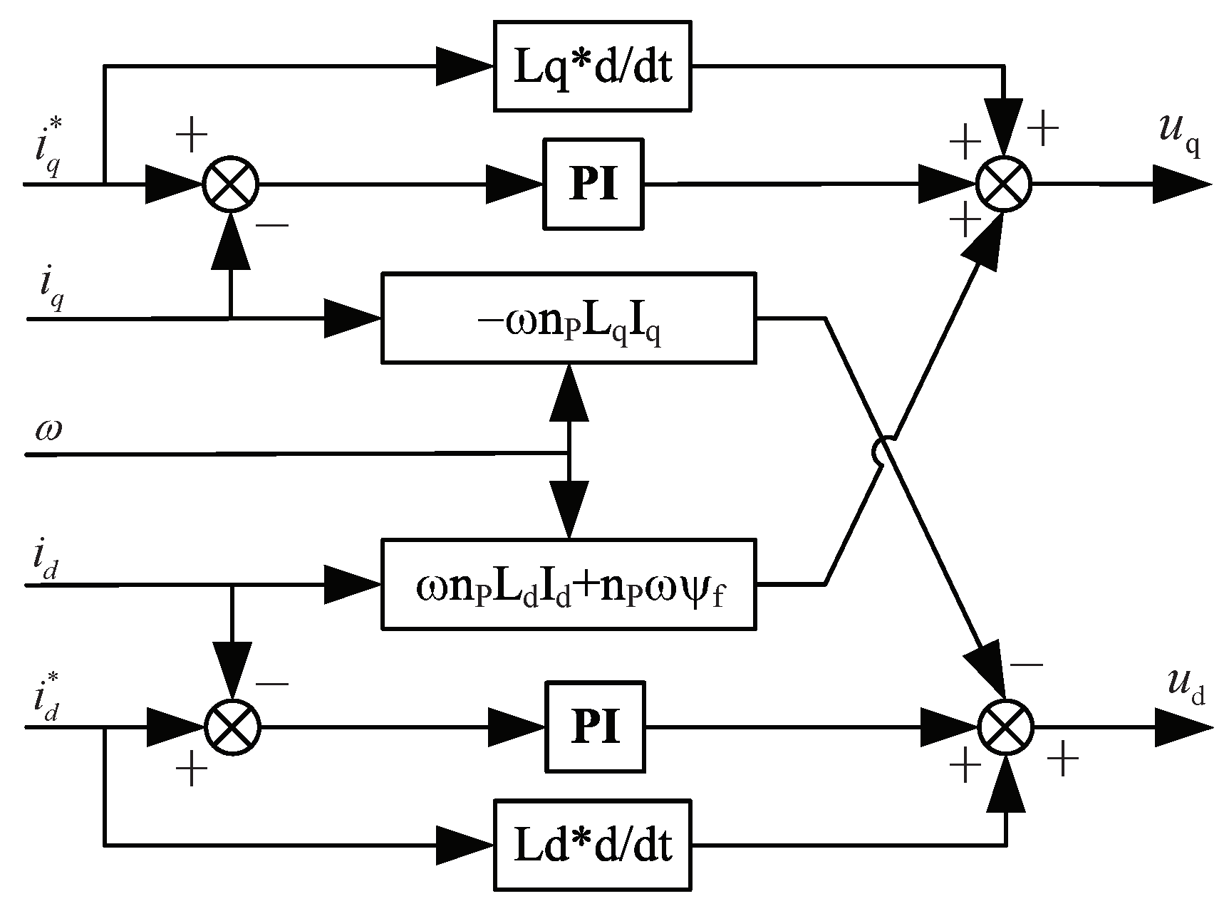
2.2. Cascade Flux-Weakening Control Framework

A cascade framework is usually used for the motor control in the industrial applications. Figure 1 shows the cascade IPMSM flux-weakening control framework, where the speed is regulated by a speed controller in the outer-loop, and the d- and q-axes currents are regulated by a current controller in the inner-loop. The d- and q-axes currents i d and i q can be obtained from the phase currents i a and i b by Clarke and Park transformations. The rotor angular velocity can be calculated from the position sensor. The reference current vector magnitude i s * is generated by the speed controller, and the d- and q-axes reference currents i d * and i q * are generated by a kind of flux-weakening algorithm. There are some different kinds of FW algorithms, such as the maximum torque per ampere (MTPA) algorithm, the maximum torque per voltage (MTPV) algorithm, the voltage-comparison based FW algorithm, etc. In this paper, the voltage-comparison based FW algorithm in used in the experimental validation. The block diagram of this algorithm is shown in Figure 2, where U d c is the DC bus voltage of the servo drive, I d m a x is the maximum amplitude of i d * and I q m a x is the maximum amplitude of i q * .
Remark 3.
Note that the nonlinear cross-coupling terms and the motor parameters’ variations are the main difficulties. No matter which flux-weakening algorithm is used, these difficulties still remain to be solved in the current controller design.
Remark 4.
In this section, the classical model of the IPMSM is used, and there is also a kind of full IPMSM model with variable parameters (in particular L d , L q and R s ) as given in [32]. In fact, directly employing the full PMSM model is another kind of solution for the problems caused by the motor parameters’ variations, and this can also improve the performance of the traditional methods, such as the integral NPC and PI. It should be pointed that using the classical model of PMSM and solving the problems in the controller design is simpler and more convenient in the existing condition. For example, the existing general servo products lack the detection of motor temperature, which is needed in the identification of L d , L q , and R s .
Remark 5.
It must be pointed out that the minus reference d-axis current must be limited in terms of its amplitude and duration in practical applications because an excessive d-axis current for a long time can demagnetize the machine [33]. Note that large current i d appears at very high speed. For the FW algorithm in actual servo products, the restriction on i d needs to be very strict for the extreme high speed operation of the motor. In the experiment at 5000 rpm in this paper, the restriction is appropriately relaxed ( I d m a x is set as −4 A) in order to test the current control performance at such extreme high speed.

3. Controller Design

Here, considering the nonlinear cross-coupling terms and parameters variations, a novel nonlinear predictive control is designed to provide the d- and q-axes stator voltages which minimize the errors between the d- and q-axes currents and their references, respectively. For convenience, the current dynamic Equation (4) can be rewritten into a standard nonlinear system as
x ˙ ( t ) = f ( x ) + g 1 u ( t ) + g 2 d ( t ) , y ( t ) = h ( x ) ,
where x, u, d, and y are respectively the state, input, disturbance, and output, given by
x = i d i q T , u = u d u q T , d = p d p q T , y = i d i q T ,
g 1 and g 2 are the input and the disturbance gain matrices, respectively, given by
g 1 = 1 L d 0 0 1 L q , g 2 = 1 L d 0 0 1 L q ,
and the functions f ( x ) and h ( x ) are given by
f ( x ) = 1 L d 0 ( R s 0 i d + n p ω L q 0 i q ) 1 L q 0 ( R s 0 i q n p ω L d 0 i d n p ω ψ f 0 ) , h ( x ) = i d i q .
To seek the best control input, a generalized cost function is defined as
J = 1 2 0 T P y ( t + τ ) y r ( t + τ ) T y ( t + τ ) y r ( t + τ ) d τ ,
where T P is the predictive period, y ( t + τ ) is the predicted output, given by
y ( t + τ ) = i d ( t + τ ) i q ( t + τ ) T ,
and y r ( t + τ ) is the desired future reference, given by
y r ( t + τ ) = i d * ( t + τ ) i q * ( t + τ ) T .

3.1. GPIO Design

The generalized proportional integral observer (GPIO) provides an adequate way to estimate the disturbance in the nonlinear system, given by
w ˙ 1 = f ( x ) + w 2 + α 1 x w 1 , w ˙ 2 = w 3 + α 2 x w 1 , w ˙ n = w n + 1 + α n x w 1 , w ˙ n + 1 = α n + 1 x w 1 ,
where w 1 , w 2 , , w n and w n + 1 are the estimations of x , d , , d ( n 1 ) and d ( n ) , respectively, and α 1 , α 2 , , α n and α n + 1 are the observer gain matrices to be designed, given by
α i = α i 1 0 0 α i 2 , i = 1 , 2 , , n + 1 .
Assumption 1.
For the nonlinear servo system (6), at least n time derivative of the disturbance d exists.
Assumption 2.
The disturbance d has constant value in steady-state, i.e., lim t d ˙ = 0 .
Disturbance can be proved to be estimated and removed from the output channel in steady-state by the following theorem.
Theorem 1.
Consider the closed-loop current nonlinear system (6). Suppose that assumptions 1 and 2 are satisfied. If the observer coefficients α 1 , α 2 , , α n and α n + 1 are tuned such that A e in Equation (17) is a Hurwitz matrix, the estimated value of disturbance w 2 can asymptotically track the actual disturbance d.
Proof. 
For the nonlinear servo system, define the disturbance estimation errors e 1 e 2 e n + 1 as
e 1 = x w 1 , e 2 = d w 2 , e n = d ( n 1 ) w n , e n + 1 = d ( n ) w n + 1 .
Denote an observer error matrix e = [ e 1 e 2 e n + 1 ] T and a disturbance matrix e = [ 0 0 d ] T . Combining the nonlinear servo system (6), the GPIO (13) and Equation (15), the derivative of e can be expressed as
e ˙ = A e e + d ˙ .
Equation (16) is an error system, where the error system matrix A e is given by
A e = α 1 I 0 0 α 2 0 I 0 α n 0 0 I α n + 1 0 0 0 ,
where I is a 2-order square matrix. The error system given by Equation (16) is asymptotically stable if A e is tuned as a Hurwitz matrix and d ˙ is bounded. This completes the proof. ☐

3.2. Output Prediction with Disturbance Compensation

With employing the GPIO, the disturbance d = p d p q T can be estimated by the estimation w 2 = p ^ d p ^ q T , where p ^ d and p ^ q are the estimated values of p d and p q . Here, to compensate the disturbance, a new input u ^ is designed as
u ^ = [ u ^ d u ^ q ] T = u + g 2 g 1 1 w 2 .
Substituting Equation (18) into Equation (6), a disturbance-compensated nonlinear servo system can be obtained, given by
x ˙ ( t ) = f ( x ) + g 1 u ^ ( t ) , y ( t ) = h ( x ) .
In addition, then, the future output of the system (19) is calculated. The input relative degree (IRD) of the system (19) is defined as σ . The future output y ( t + τ ) is predicted by Taylor series expansion
y ( t + τ ) y ( t ) + τ y [ 1 ] ( t ) + + τ σ + r ( σ + r ) ! y [ σ + r ] ( t ) ,
where r is the control order (see [27] for detailed definition). The input relative degree (IRD) σ is equal to 1, and the control order r is chosen as 0. Hence, the output y and its derivative are given by
y ( t ) = L f 0 h ( x ) , y ˙ ( t ) = L f 1 h ( x ) + L g 1 h ( x ) u ^ ,
where
L f 0 h ( x ) = h ( x ) = i d i q T , L f 1 h ( x ) = ( h ( x ) ) x f ( x ) = f ( x ) , L g 1 h ( x ) = ( h ( x ) ) x g ( x ) = 1 L d 0 0 1 L q .
In addition, then, the predicted output array can be obtained, given by
y ¯ ( t + τ ) = Γ y ( t ) y ˙ ( t ) ,
where Γ ( τ ) is a weighting matrix, given by
Γ ( τ ) = 1 0 τ 0 0 1 0 τ .

3.3. Receding Optimization and Control Law Design

Similarly to Equation (23), the reference output array can be obtained, given by
y ¯ r ( t + τ ) = Γ y r ( t ) y ˙ r ( t ) ,
Let Γ ¯ = 0 T P Γ T ( τ ) Γ ( τ ) d τ , and the ( i , j ) th element of Γ ¯ is given by
Γ ¯ ( T ) i , j = 1 ( i 1 ) ! ( j 1 ) ! ( i + j 1 ) T P 0 0 T P i + j 1 , i , j = 1 , 2 .
By virtue of Equations (23)–(26), the performance index (10) is expressed as
J = 1 2 y ¯ ( t ) y ¯ r ( t ) T Γ ¯ ( T ) y ¯ ( t ) y ¯ r ( t ) .
Let ( J / u ^ d ) = 0 and ( J / u ^ q ) = 0 . Then, the optimized input u ^ which minimizes the cost function (27) is obtained as
u ^ = g 1 ( x ) K M ρ + L f 1 h ( x ) y ˙ r ,
where
g ( x ) = L g 1 h ( x ) = ( h ( x ) ) x g 1 ( x ) = 1 L d 0 0 1 L q , M ρ = i d i d * i q i q * , y r = i d * i q * .
Combining Equations (18) and (28), an optimized and disturbance-compensated control input is finally obtained, given by
u = [ u d u q ] T = g 1 ( x ) K M ρ + L f 1 h ( x ) y ˙ r g 2 g 1 1 w 2 .

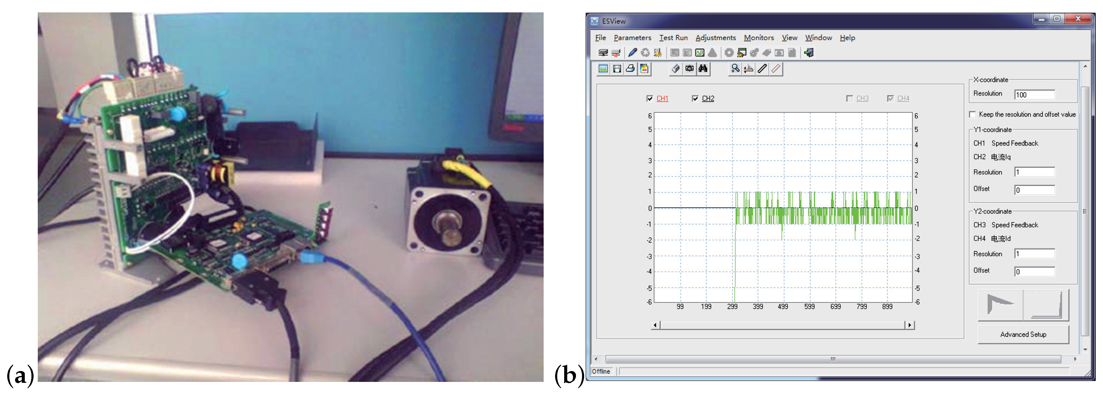
4. Experimental Validation

In this section, a series of experiments are conducted on a DSP-based IPMSM servo system. The experiment platform is showed in Figure 3. The processor chip of the experimental drive is a fixed-point DSP (TMS3202812 made by Texas Instruments, Dallas, TX, United States). The PWM period is set as 100 μ s, and the dead-time is set as 3.2 μ s. The power driving circuit consists of a single-phase of diode bridge rectifier, a large capacitor filter, and an IGBT inverter. The DC link voltage is 310 V. The phase currents are measured by the Hall-effect devices, and the position of the rotor is measured by the 17-bit absolute encoder. The experimental motor is an eight-pole IPMSM, and the nominal parameters are shown in Table 1.
To illustrate the superiority of the proposed control method (NPC + GPIO), experiments have been carried out compared with the integral nonlinear predictive control (NPC + I) and the improved proportional integral (PI) control. The control performances of these controllers against the nonlinear cross-coupling terms and the motor parameters’ variations have been tested in current control mode and speed control mode respectively, to reflect the different working conditions of the motor and obtain fair comparisons.
Remark 6.
Using two integrators to compensate the disturbance d, the control of NPC + I is given by
u = [ u d u q ] T = g 1 ( x ) K M ρ + L f 1 h ( x ) y ˙ r g 2 g 1 1 y I ,
where
y I = K I d 0 0 K I q 0 t ( y y r ) d t .
Remark 7.
The performance of the basic PI for flux-weakening current control is bad. Hence, the basic PI control is improved by a voltage feedforward decoupling compensation. Figure 4 shows the diagram of such improved PI current control.

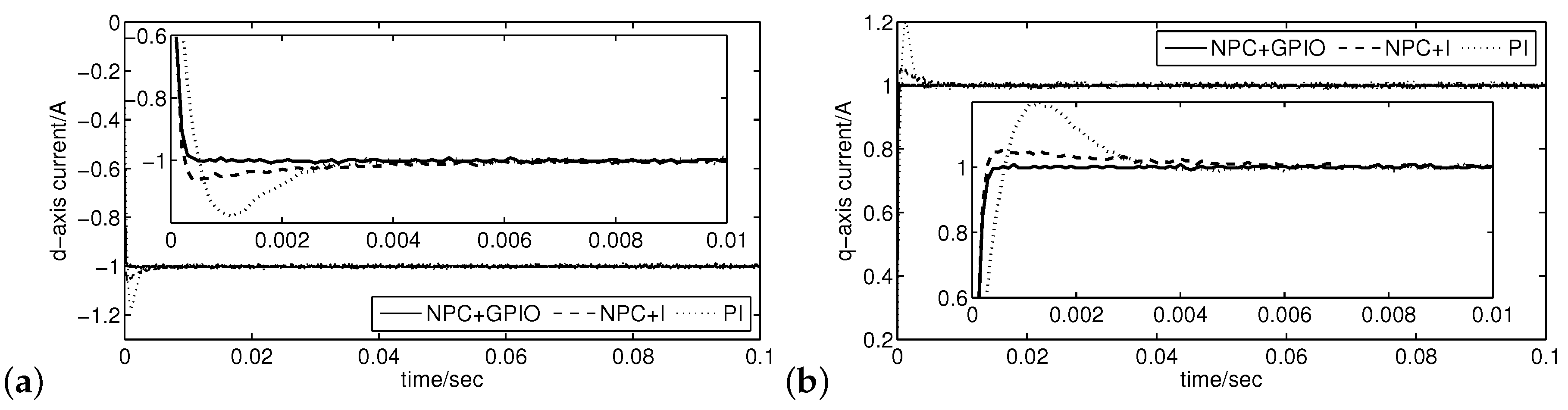
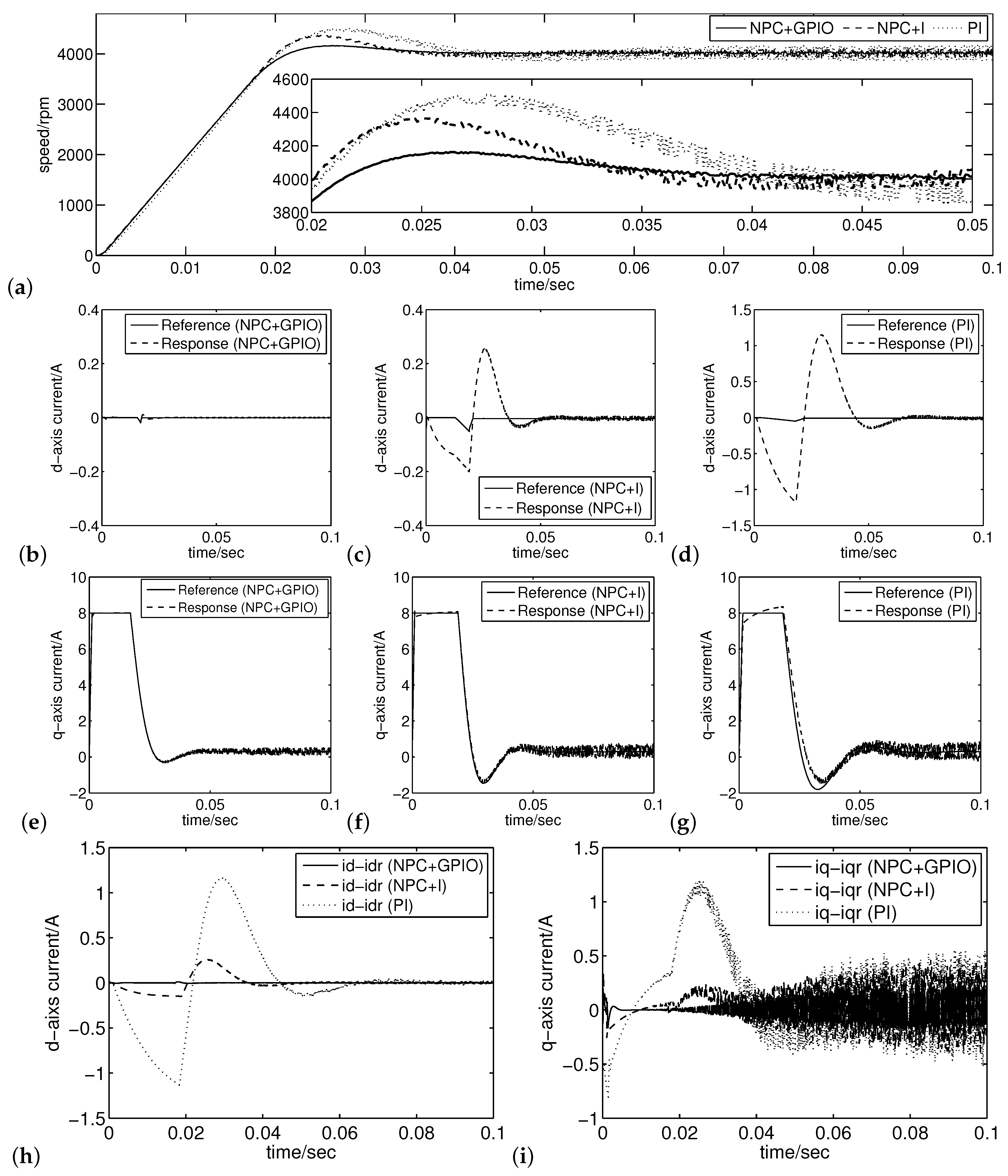
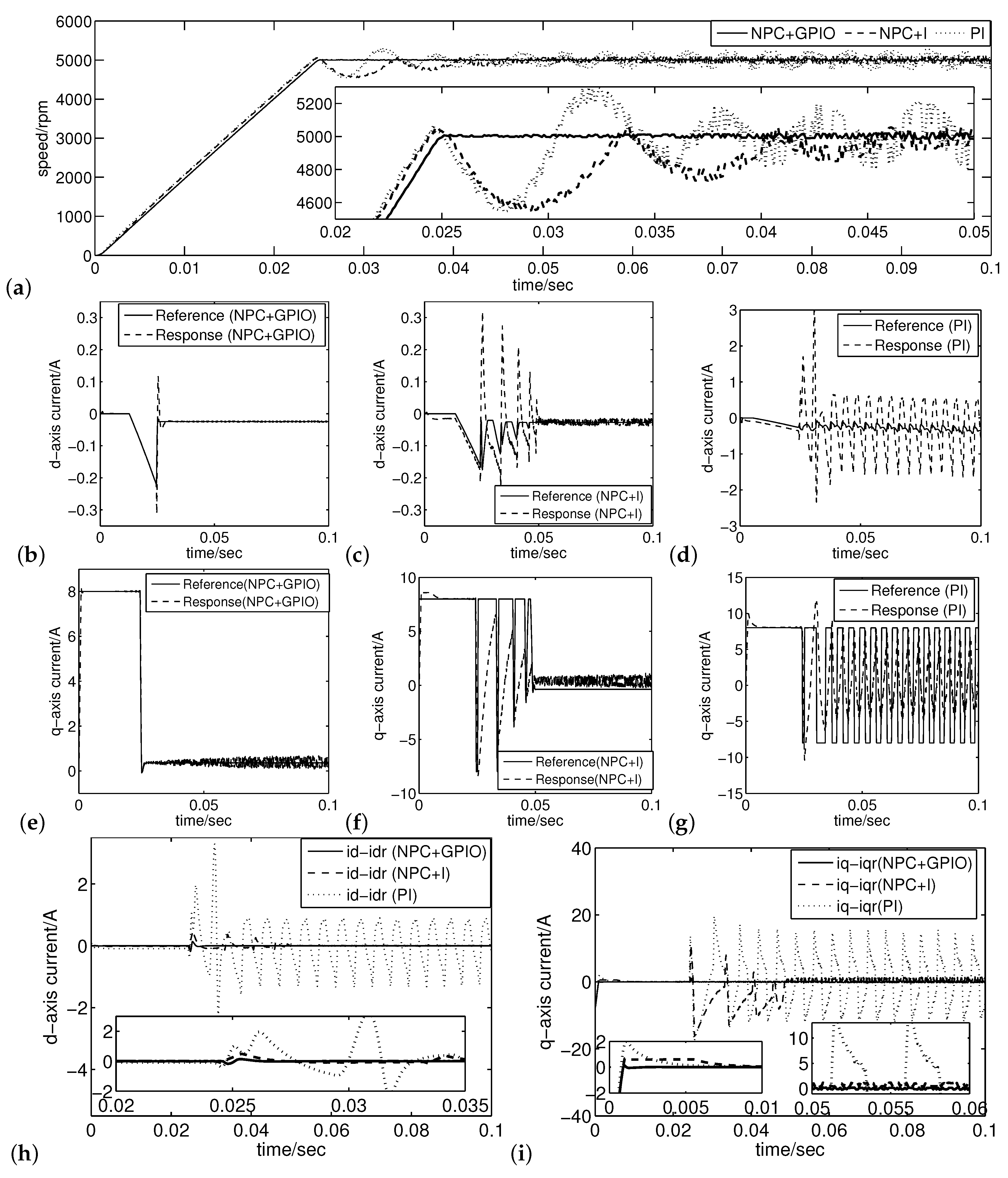
4.1. Control Performance under Current Control Model

In this subsection, the control performances against the nonlinear cross-coupling terms and the motor parameters’ variations are tested under current control model, where the reference d- and q-axes currents are directly given and the speed loop of the IPMSM does not work. The control parameters are tuned and shown in Table 2.
Figure 5 and Figure 6 respectively show the current step response curves in the case of the nominal mode and in the case of model parameters variations, under the three controllers. The case of nominal model is defined that the nominal motor parameters from Table 1 are used into tuning the parameters of the controllers, and this case is designed to independently test the performance against the nonlinear cross-coupling terms. In addition, then, the case of motor parameters’ variations is defined that inaccurate motor parameters are used, and this case is designed to test the performances against both the nonlinear cross-coupling terms and the motor parameters. The inaccurate motor parameters are set as that L d , L q , and ψ f decrease by 30%, and R s increases by 100%. Figure 5 and Figure 6 both show that the proposed NPC + GPIO controller has a smallest overshoot and a shortest settling time as compared with the NPC + I controller and the PI controller no matter in the case of nominal model or in the case of motor parameters’ variations. The concrete dynamic-state and steady-state performance indices in the two cases are respectively given in Table 3 and Table 4. It is also observed that the proposed NPC + GPIO controller has a smallest offset error and a smallest fluctuation rate in the two cases. Hence, the proposed NPC + GPIO controller shows the best dynamic-state and steady-state performances as compared with the NPC + I controller and PI controller no matter in the case of nominal model or in the case of motor parameters’ variations. With the motor parameters varying, the proposed NPC + GPIO controller also maintains the best performances, while the NPC + I controller and PI controller both face the deterioration of control performances.
Remark 8.
A direct experimental method to realize manually-adjustable model parameters variations is putting the motor into a thermostat to keep a constant high temperature, and then using precise instruments to read the new values of R s , L d , L q , and ψ f . This method is very difficult to realize, and, moreover, the values of L d , L q are related to not only the temperature, but also the d- and q-axes currents, the winding current frequency, and the rotor angular. Thus, the manually-adjustable model parameters variations are almost impossible to be exactly realized by the direct experimental means. In this paper, the model parameters’ variations are realized by tuning the corresponding parameters of the controllers far from their nominal values. This indirect experimental method is easily realized and still effective.

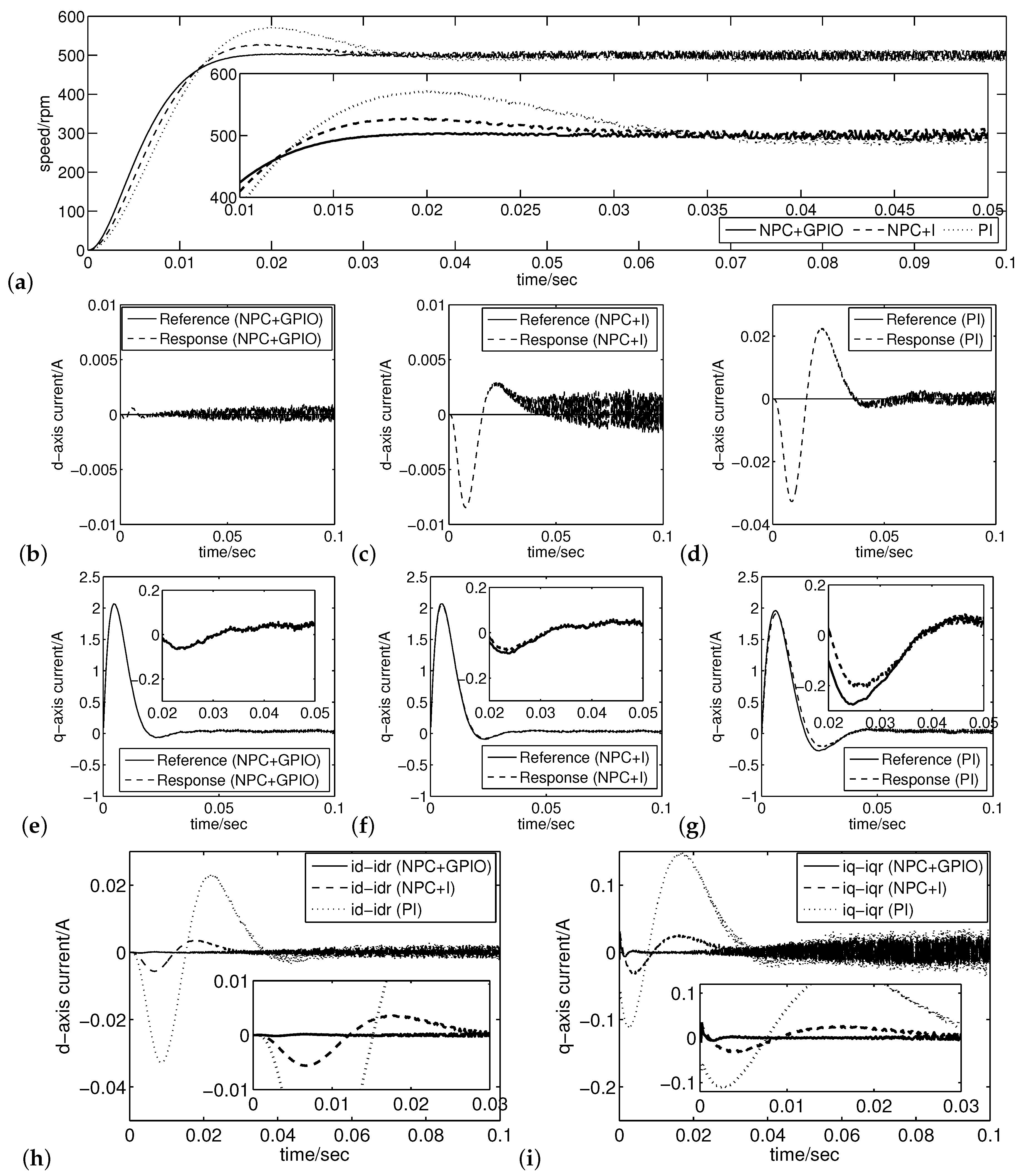
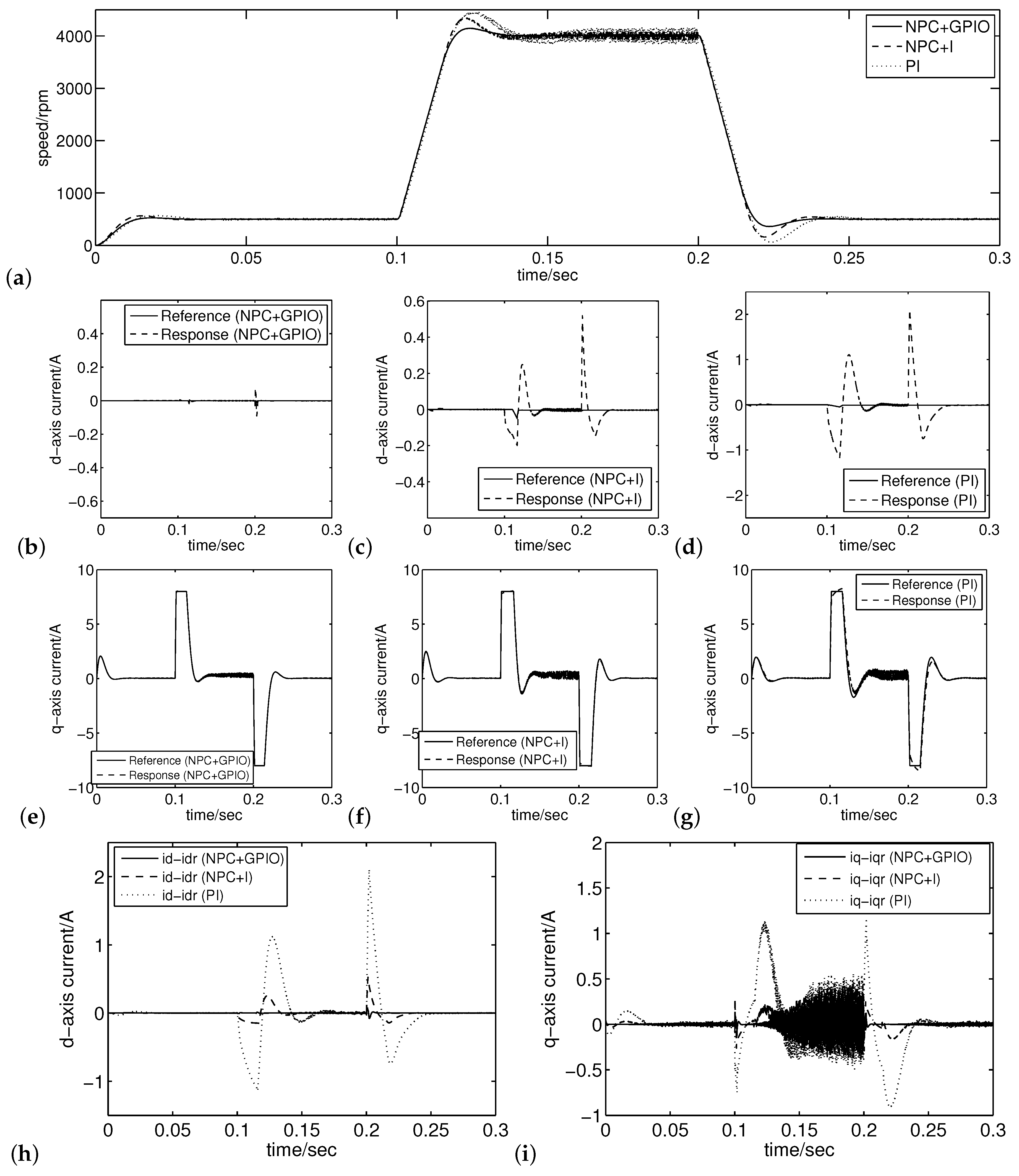
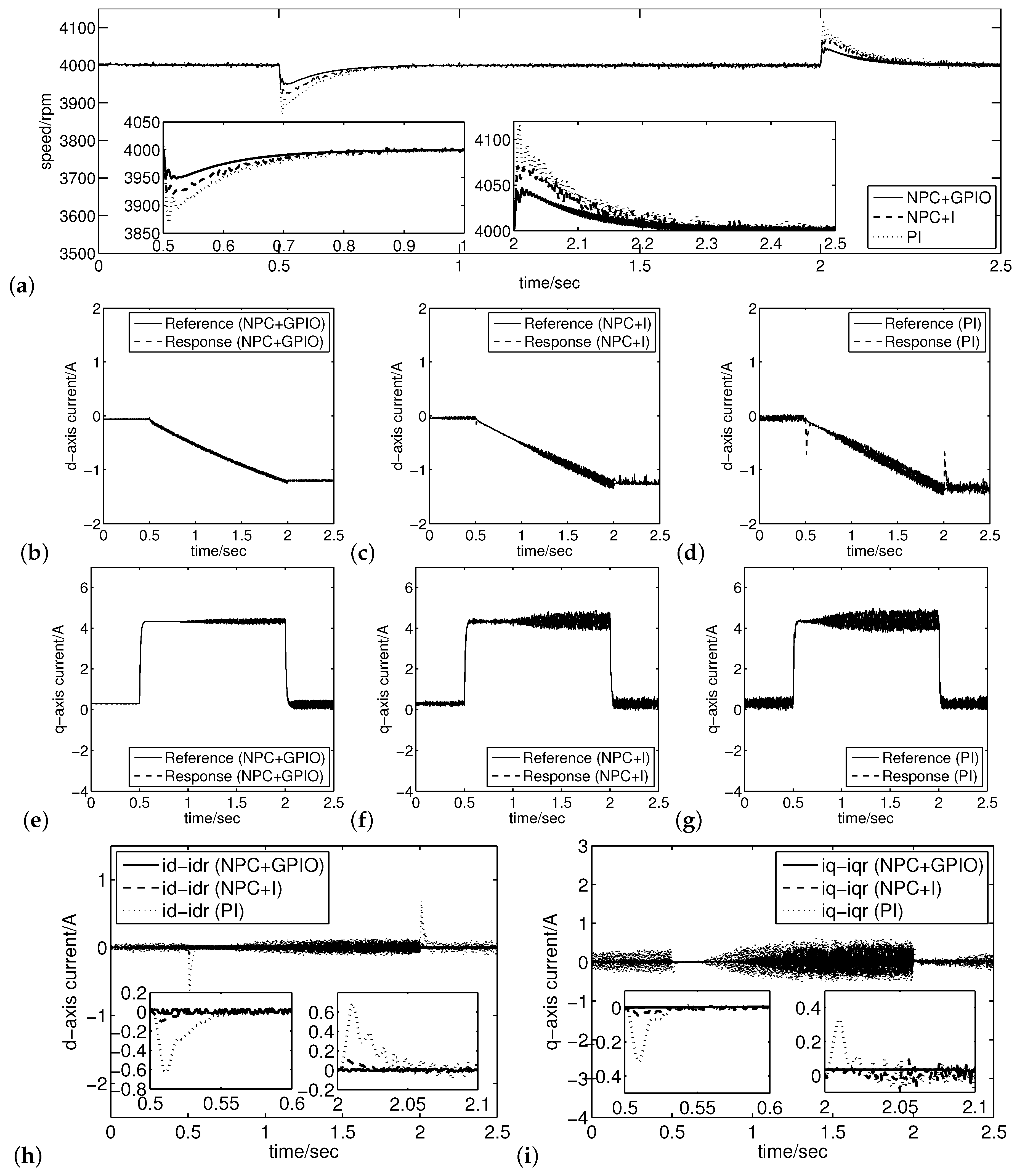
4.2. Control Performance under Speed Control Mode

In the previous subsection, the outer-loop speed controller does not work, and the inner-loop current control performances of the NPC + GPIO, NPC + I and PI controllers are independently tested. In this subsection, the outer-loop speed control performance is tested by using the same speed controller (PI) and different current controllers, to investigate the improvement of the outer-loop control performance by just improving the inner-loop control performance. The experimental conditions are set so that the motor faces the same model parameters’ variations as the previous subsection, and the same control parameters of the current controllers as the previous subsection are used. For the outer-loop speed control, parameters of the PI controller are chosen as K p = 0 . 03 and K i = 30 .
Figure 7, Figure 8 and Figure 9 show the speed and current responses with operation speeds at 500 rpm, 4000 rpm and 5000 rpm, respectively, under the same speed controller (PI) and the different current controllers. At the operation speeds of 500 rpm, the motor is in the CT region, and, at speeds 4000 rpm and 5000 rpm (maximum speed), the motor is mainly in the FW region. With the operation speed at 500 rpm, it is clearly observed from Figure 7a that the proposed NPC + GPIO inner-loop controller realizes a faster and smoother outer-loop speed dynamic process as compared with the NPC + I and the PI controllers. The corresponding d- and q-axes current responses are shown in Figure 7b–g. To be more clear, the d- and q-axes current-tracking errors are given in Figure 7h–i, where one can find that the NPC + GPIO has the best current-tracking performances. In addition, then, with the operation speeds at 4000 rpm and 5000 rpm, Figure 8a and Figure 9a show that the proposed NPC + GPIO inner-loop controller maintains a good speed dynamic performance, while the NPC + I or the PI inner-loop controller faces the significant performance degradation. The corresponding current responses and current-tracking errors are shown in Figure 8b–i and Figure 9b–i. In addition, the proposed NPC + GPIO controller has the best current-tracking performances. The concrete speed-tracking performance indices are given in Table 5, and the proposed NPC + GPIO current controller also has a smallest speed offset error and a smallest speed fluctuation rate.
With the operation speed at 500 rpm, it is clearly observed from Figure 7a that the proposed NPC + GPIO inner-loop controller realizes a faster and smoother outer-loop speed dynamic process as compared with the NPC + I and the PI controllers. The corresponding d- and q-axes current responses are shown in Figure 7b–g. To be more clear, the d- and q-axes current-tracking errors are given in Figure 7h–i, where one can find that the NPC + GPIO has the best current-tracking performances. In addition, then, with the operation speeds at 4000 rpm and 5000 rpm, Figure 8a and Figure 9a show that the proposed NPC + GPIO inner-loop controller maintains a good speed dynamic performance, while the NPC + I or the PI inner-loop controller faces the significant performance degradation. The corresponding current responses and current-tracking errors are shown in Figure 8 and Figure 9b–i. In addition, the proposed NPC + GPIO controller has the best current-tracking performances. The concrete speed-tracking performance indices are given in Table 5, and also the proposed NPC + GPIO current controller has a smallest speed offset error and a smallest speed fluctuation rate.
Figure 10 shows the speed and current responses with operation speed at 500 rpm–4000 rpm–500 rpm, to reflect the control performance in the case of transition between the CT and FW regions. It is clearly observed from Figure 10a that the proposed NPC + GPIO inner-loop controller realizes a fastest and smoothest transition process between the CT region (around 500 rpm) and FW region (around 4000 rpm). The corresponding d- and q-axes current responses are shown in Figure 10b–i, and one can find that the NPC + GPIO also has the best current-tracking performances. The fastest and smoothest transition process between the CT and FW regions mainly benefits from the improvement of current-tracking performances.
Finally, performance in the case of load disturbance is tested. When the motor is running at a steady state, the load torque is added suddenly and removed suddenly after some duration. Figure 11 and Figure 12 respectively show the responses with operation speed at 500 rpm (in CT region) in the case of 2.4 N·m load torque (nominal torque), and 4000 rpm in the case of 1.5 N·m load torque (nominal power), respectively. It can be observed from Figure 11a and Figure 12a that the proposed NPC + GPIO maintains a best speed dynamic performance in the case of load in both CT and FW regions. In addition, the speed dynamic performance in the case of load is improved because current-tracking performances as shown in Figure 11b–i and Figure 12b–i are first improved.
In brief, with using the same outer-loop speed controller and just the different inner-loop current controllers, the proposed NPC + GPIO current controller realizes the best speed-tracking performance in different cases. Moreover, from the CT region to the FW region, the proposed NPC + GPIO current controller maintains a good speed performance, while the NPC + I or the improved PI faces the significant performance degradation.
Remark 9.
In Figure 8b–g and Figure 9b–g, it is observed that the reference d- and q-axes currents of the three different current controllers are different. Actually, in the flux-weakening algorithm employed in this paper, the reference d- and q-axes currents relate to the outputs of the current controller.
Remark 10.
In Table 5, t s of the PI current controller (with operation speed at 5000 rpm) is not given since there always exists speed-tracking errors more than 5%. Therefore, bad current-tracking performances make the flux-weakening speed control fail.
Remark 11.
In Figure 9a (with operation speed at 5000 rpm), it can be observed that oscillations occur at steady-state speeds under the NPC + I and PI, and they are weak in Figure 8a (with operation speed at 4000 rpm). Note that 5000 rpm is the maximum limit speed of this motor which does not generally appear in the actual working condition, and the original reason for this experimental phenomenon is that the current control problems (nonlinear cross-coupling terms and motor parameters’ variations) become the most serious. On the one hand, the minus reference d-axis current is calculated by the FW algorithm to reduce the stator voltage and increase the motor speed further, and if the d-axis current tracks its reference very well (see Figure 9b), the speed response will be very smooth. However, if the d-axis current response has some oscillation (see Figure 9c,d), this kind of oscillation will also occur in the speed response. On the other hand, since the d- and q-axes currents’ responses have some oscillations, the mechanical torque will also have some corresponding oscillation, and this will also lead to the oscillation in speed response.

5. Conclusions

In this paper, a GPIO-based NPC has been designed for the IPMSM servo system to improve the FW current control performance against the complex nonlinear cross-coupling terms and the IPMSM parameters’ variations. A comparison of the integral NPC scheme and the improved PI control scheme has proved its superiority. Experiments under the current and speed control modes have been respectively conducted on a DSP-based IPMSM servo system. The results have validated that the proposed control scheme can obtain a satisfactory FW control performance.

Author Contributions

C.W. conceived the main idea, performed experiments, and wrote the manuscript. J.Y. contributed to developing the idea in this research. C.W., J.Y. and Q.L. thoroughly revised the paper. All authors have read and agreed to the published version of the manuscript.

Acknowledgments

The authors would like to thank the reviewers for their very helpful comments and suggestions which have improved the presentation of the paper. This work was supported in part by the National Aerospace Science Foundation of China under Grant 2018286900.

Conflicts of Interest

The authors declare no conflict of interest.

References

  1. Lee, S.; Kim, K.; Cho, S.; Jang, J.; Lee, T.; Hong, J. Optimal design of interior permanent magnet synchronous motor considering the manufacturing tolerances using Taguchi robust design. IET Electr. Power Appl. 2014, 8, 23–28. [Google Scholar] [CrossRef]
  2. Kwon, T.S.; Sul, S.K. Novel antiwindup of a current regulator of a surface-mounted permanent-magnet motor for flux-weakening control. IEEE Trans. Ind. Appl. 2006, 42, 1293–1300. [Google Scholar] [CrossRef]
  3. Sue, S.; Pan, C. Voltage-constraint-tracking-based field-weakening control of IPM synchronous motor drives. IEEE Trans. Ind. Electron. 2008, 55, 340–347. [Google Scholar] [CrossRef]
  4. Andreescu, G.; Pitic, C.; Blaabjerg, F.; Boldea, I. Combined flux observer with signal injection enhancement for wide speed range sensorless direct torque control of IPMSM drives. IEEE Trans. Energy Convers. 2008, 23, 393–402. [Google Scholar] [CrossRef]
  5. Huynh, T.; Hsieh, M. Performance analysis of permanent magnet motors for electric vehicles (EV) traction considering driving cycles. Energies. 2018, 11, 1385. [Google Scholar] [CrossRef] [Green Version]
  6. Ren, J.; Liu, Y.; Wang, N.; Liu, S. Sensorless control of ship propulsion interior permanent magnet synchronous motor based on a new sliding mode observer. ISA Trans. 2015, 54, 15–26. [Google Scholar] [CrossRef] [PubMed]
  7. Kwon, T.; Choi, G.; Kwak, M.; Sul, S. Novel flux-weakening control of an IPMSM for quasi-six-step operation. IEEE Trans. Ind. Appl. 2008, 44, 1722–1731. [Google Scholar] [CrossRef]
  8. Wang, G.; Yang, R.; Xu, D. DSP-based control of sensorless IPMSM drives for wide-speed-range operation. IEEE Trans. Ind. Electron. 2013, 60, 720–727. [Google Scholar] [CrossRef]
  9. Ishikawa, T.; Yamada, M.; Kurita, N. Design of magnet arrangement in interior permanent magnet synchronous motor by response surface methodology in consideration of torque and vibration. IEEE Trans. Magn. 2011, 47, 1290–1293. [Google Scholar] [CrossRef]
  10. Park, C.; Lee, J. A torque error compensation algorithm for surface mounted permanent magnet synchronous machines with respect to magnet temperature variations. Energies 2017, 10, 1365. [Google Scholar] [CrossRef]
  11. Jung, S.; Hong, J.; Nam, K. Current minimizing torque control of the IPMSM using Ferrari’s method. IEEE Trans. Power Electron. 2013, 28, 5603–5617. [Google Scholar] [CrossRef]
  12. Tang, M.; Zhuang, S. On speed control of a permanent magnet synchronous motor with current predictive compensation. Energies 2019, 12, 65. [Google Scholar] [CrossRef] [Green Version]
  13. Park, Y.; Koo, M.; Jang, S.; Choi, J.; You, D. Dynamic characteristic analysis of interior permanent magnet synchronous motor considering varied parameters by outer disturbance based on electromagnetic field analysis. IEEE Trans. Magn. 2014, 50, 1–4. [Google Scholar] [CrossRef]
  14. Preindl, M.; Bolognani, S. Model predictive direct torque control with finite control set for PMSM drive systems, part 2: Field weakening operation. IEEE Trans. Ind. Inf. 2008, 23, 393–402. [Google Scholar] [CrossRef]
  15. Liu, H.; Li, S. Speed control for PMSM servo system using predictive functional control and extended state observer. IEEE Trans. Ind. Electron. 2012, 59, 1171–1183. [Google Scholar] [CrossRef]
  16. Li, X.; Li, S. Speed control for a PMSM servo system using model reference adaptive control and an extended state observer. J. Power Electron. 2014, 14, 549–563. [Google Scholar] [CrossRef] [Green Version]
  17. Shi, J.; Li, S. Analysis and compensation control of dead-time effect on space vector PWM. J. Power Electron. 2015, 15, 431–442. [Google Scholar] [CrossRef] [Green Version]
  18. Wang, H.; Li, S.; Yang, J.; Zhou, X. Continuous sliding mode control for permanent magnet synchronous motor speed regulation systems under time-varying disturbances. J. Power Electron. 2016, 16, 1324–1335. [Google Scholar] [CrossRef] [Green Version]
  19. Mengoni, M.; Zarri, L.; Tani, A.; Serra, G.; Casadei, D. A comparison of four robust control schemes for field-weakening operation of induction motors. IEEE Trans. Power Electron. 2012, 27, 307–320. [Google Scholar] [CrossRef]
  20. Morimoto, S.; Sanada, M.; Takeda, Y. Wide-speed operation of interior permanent magnet synchronous motors with high-performance current regulator. IEEE Trans. Ind. Electron. 1994, 30, 920–926. [Google Scholar] [CrossRef]
  21. Zhou, K.; Ai, M.; Sun, D.; Jin, N.; Wu, X. Field weakening operation control strategies of PMSM based on feedback linearization. Energies 2019, 12, 4526. [Google Scholar] [CrossRef] [Green Version]
  22. Chen, J.; Li, J.; Qu, R. Maximum-torque-per-ampere and magnetization-state control of a variable-flux permanent magnet machine. IEEE Trans. Ind. Electron. 2017, 65, 1158–1169. [Google Scholar] [CrossRef]
  23. Mynar, Z.; Vesely, L.; Vaclavek, P. PMSM model predictive control with field-weakening implementation. IEEE Trans. Ind. Electron. 2016, 63, 5156–5166. [Google Scholar] [CrossRef]
  24. Fliess, M.; Lévine, J.; Martin, P.; Rouchon, P. Flatness and defect of nonlinear systems: Introductory theory and examples. Int. J. Control 1995, 61, 1327–1361. [Google Scholar] [CrossRef] [Green Version]
  25. Chen, W.-H.; Yang, J.; Guo, L.; Li, S. Disturbance-observer-based control and related methods—An overview. IEEE Trans. Ind. Electron. 2015, 63, 1083–1095. [Google Scholar] [CrossRef] [Green Version]
  26. Yang, J.; Chen, W.-H.; Li, S.; Guo, L.; Yan, Y. Disturbance/uncertainty estimation and attenuation techniques in pmsm drives—A survey. IEEE Trans. Ind. Electron. 2016, 64, 3273–3285. [Google Scholar] [CrossRef] [Green Version]
  27. Chen, W.; Ballance, D.; Gawthrop, P. Optimal control of nonlinear systems: A predictive control approach. Automatica 2013, 39, 633–641. [Google Scholar] [CrossRef] [Green Version]
  28. Errouissi, R.; Ouhrouche, M.; Chen, W.; Trzynadlowski, A. Robust cascaded nonlinear predictive control of a permanent magnet synchronous motor with antiwindup compensator. IEEE Trans. Ind. Electron. 2012, 59, 3078–3088. [Google Scholar] [CrossRef]
  29. Yang, J.; Zheng, W. Offset-free nonlinear MPC for mismatched disturbance attenuation with application to a static var compensator. IEEE Trans. Circuits Syst. II Express Briefs 2014, 61, 49–53. [Google Scholar] [CrossRef]
  30. Yang, J.; Zheng, W.; Li, S.; Wu, B.; Cheng, M. Design of a prediction-accuracy-enhanced continuous-time MPC for disturbed systems via a disturbance observer. IEEE Trans. Ind. Electron. 2015, 62, 5807–5816. [Google Scholar] [CrossRef]
  31. Wu, C.; Yang, J.; Li, S.; Li, Q.; Guo, L. Disturbance observer based model predictive control for accurate atmospheric entry of spacecraft. Adv. Space Res. 2018, 61, 2457–2471. [Google Scholar] [CrossRef]
  32. Quintal-Palomo, R.E.; Gwozdziewicz, M.; Dybkowski, M. Modelling and co-simulation of a permanent magnet synchronous generator. COMPEL Int. J. Comp. Math. Electr. Electron. 2019, 38, 1904–1917. [Google Scholar] [CrossRef]
  33. Quintal-Palomo, R.E. Analysis of Current Signals in a Partially Demagnetized Vector Controlled Interior Permanent Magnet Generator. Power Electron. Drives 2019, 4, 179–190. [Google Scholar] [CrossRef] [Green Version]
Figure 1. Block diagram of the interior permanent magnet synchronous motor (IPMSM) flux-weakening cascaded control framework.
Energies 13 01716 g001
Figure 2. Voltage-comparison based flux-weakening algorithm.
Energies 13 01716 g002
Figure 3. The experiment platform: (a) the tested IPMSM servo system; (b) the software interface of the upper computer.
Energies 13 01716 g003
Figure 4. Current control based on the improved PI control.
Energies 13 01716 g004
Figure 5. D- and q-axes current step response curves (the reference d-axis current is −1 A and the reference q-axis current is 1 A) in the case of nominal model under the proposed controller (NPC + GPIO), the integral controller (NPC + I) and the improved PI controller: (a) d-axis; (b) q-axis.
Energies 13 01716 g005
Figure 6. D- and q-axes current step response curves (the reference d-axis current is −1 A and the reference q-axis current is 1 A) in the case of model parameters variations under the proposed controller (NPC + GPIO), the integral controller (NPC + I) and the improved PI controller: (a) d-axis; (b) q-axis.
Energies 13 01716 g006
Figure 7. Speed and current responses with operation speed at 500 rpm under the same speed controller (PI) and the different current controllers (the proposed controller (NPC + GPIO), the integral controller (NPC + I) and the improved PI controller): (a) speed responses; (b) d-axis current response under the proposed controller; (c) d-axis current response under the integral controller; (d) d-axis current response under the PI controller; (e) q-axis current response under the proposed controller; (f) q-axis current response under the integral controller; (g) q-axis current response under the PI controller; (h) d-axis current-tracking errors under the different current-controllers (the d-axis response current (id) minus the d-axis reference current (idr)); (i) q-axis current-tracking errors under the different current controllers (the q-axis response current (iq) minus the q-axis reference current (iqr)).
Energies 13 01716 g007
Figure 8. Speed and current responses with operation speed at 4000 rpm under the same speed controller (PI) and the different current controllers (the proposed controller (NPC + GPIO), the integral controller (NPC + I) and the improved PI controller): (a) speed responses; (b) d-axis current response under the proposed controller; (c) d-axis current response under the integral controller; (d) d-axis current response under the PI controller; (e) q-axis current response under the proposed controller; (f) q-axis current response under the integral controller; (g) q-axis current response under the PI controller; (h) d-axis current-tracking errors under the different current controllers (the d-axis response current (id) minus the d-axis reference current (idr)); (i) q-axis current-tracking errors under the different current controllers (the q-axis response current (iq) minus the q-axis reference current (iqr)).
Energies 13 01716 g008
Figure 9. Speed and current responses with operation speed at 5000 rpm under the same speed controller (PI) and the different current controllers (the proposed controller (NPC + GPIO), the integral controller (NPC + I) and the improved PI controller): (a) speed responses; (b) d-axis current response under the proposed controller; (c) d-axis current response under the integral controller; (d) d-axis current response under the PI controller; (e) q-axis current response under the proposed controller; (f) q-axis current response under the integral controller; (g) q-axis current response under the PI controller; (h) d-axis current-tracking errors under the different current controllers (the d-axis response current (id) minus the d-axis reference current (idr)); (i) q-axis current-tracking errors under the different current controllers (the q-axis response current (iq) minus the q-axis reference current (iqr)).
Energies 13 01716 g009
Figure 10. Speed and current responses with operation speed at 500 rpm–4000 rpm–500rpm under the same speed controller (PI) and the different current controllers (the proposed controller (NPC + GPIO), the integral controller (NPC + I) and the improved PI controller): (a) speed responses; (b) d-axis current response under the proposed controller; (c) d-axis current response under the integral controller; (d) d-axis current response under the PI controller; (e) q-axis current response under the proposed controller; (f) q-axis current response under the integral controller; (g) q-axis current response under the PI controller; (h) d-axis current-tracking errors under the different current controllers (the d-axis response current (id) minus the d-axis reference current (idr)); (i) q-axis current-tracking errors under the different current controllers (the q-axis response current (iq) minus the q-axis reference current (iqr)).
Energies 13 01716 g010
Figure 11. Speed and current responses with operation speed at 500 rpm in the case of 2.4 N·m load torque (nominal torque) under the same speed controller (PI) and the different current controllers (the proposed controller (NPC + GPIO), the integral controller (NPC + I) and the improved PI controller): (a) speed responses; (b) d-axis current response under the proposed controller; (c) d-axis current response under the integral controller; (d) d-axis current response under the PI controller; (e) q-axis current response under the proposed controller; (f) q-axis current response under the integral controller; (g) q-axis current response under the PI controller; (h) d-axis current-tracking errors under the different current controllers (the d-axis response current (id) minus the d-axis reference current (idr)); (i) q-axis current-tracking errors under the different current controllers (the q-axis response current (iq) minus the q-axis reference current (iqr)).
Energies 13 01716 g011
Figure 12. Speed and current responses with operation speed at 4000 rpm in the case of 1.5 N·m load torque (nominal power) under the same speed controller (PI) and the different current controllers (the proposed controller (NPC + GPIO), the integral controller (NPC + I) and the improved PI controller): (a) speed responses; (b) d-axis current response under the proposed controller; (c) d-axis current response under the integral controller; (d) d-axis current response under the PI controller; (e) q-axis current response under the proposed controller; (f) q-axis current response under the integral controller; (g) q-axis current response under the PI controller; (h) d-axis current-tracking errors under the different current controllers (the d-axis response current (id) minus the d-axis reference current (idr)); (i) q-axis current-tracking errors under the different current controllers (the q-axis response current (iq) minus the q-axis reference current (iqr)).
Energies 13 01716 g012
Table 1. Motor nominal parameters.
ParametersValueParametersValue
Rated power P750 (W)Stator inductance on d axis L d 3.5 (mH)
Rated voltage U N 200 (V)Stator inductance on q axis L q 4 (mH)
Rated current I N 4.5 (A)Rotor inertia J N 1.76 × 10 4  (kg· m2)
Rated torque T N 2.4 (Nm)Stator resistance R s 1.74 ( Ω )
Rated speed n N 3000 (rpm)Flux linkage ψ f 0.1267 (Wb)
Maximum speed n max 5000 (rpm)Torque constant K t 0.5422 (Nm/A)
Pole pairs n P 4Viscous coefficient B7.388 × 10 5  (Nm · s/rad)
Table 2. Parameters of the three current controllers.
Current ControllerControl Parameters
NPC + GPIOGPIO order = 4, α 1 = 32 0 0 32 , α 2 = 384 0 0 384 , α 3 = 2048 0 0 2048 , α 4 = 4096 0 0 4096
R s , L d , L q and ψ f are tuned to be nominal or inaccurate respectively in the two cases
NPC + I K I d = 3000 , K I q = 3000
R s , L d , L q and ψ f are also tuned to be nominal or inaccurate respectively in the two cases
PI K P d = 36 , K I d = 3000 , K P q = 36 , K I q = 3000 (subscripts d and q mean d- or q- axis, respectively)
R s , L d , L q and ψ f are also tuned to be nominal or inaccurate respectively in the two cases
Table 3. Comparison of current-tracking performance indices in the case of nominal model.
Speed Controllerd- or q-AxisCurrent ControllerDynamic-StateSteady-State
OS (%) t s (ms)Offset Error (mA)Fluctuation Rate (%)
d-axisNPC + GPIO0.250.600.83
NPC + I6.363.400.94
PI17.993.101.25
q-axisNPC + GPIO0.830.602.78
NPC + I5.274.103.13
PI19.933.004.17
Table 4. Comparison of current-tracking performance indices in the case of model parameters variations.
Speed Controllerd- or q-AxisCurrent ControllerDynamic-StateSteady-State
OS (%) t s (ms)Offset Error (mA)Fluctuation Rate (%)
d-axisNPC + GPIO1.760.600.86
NPC + I6.365.051.30.97
PI29.113.542.21.32
q-axisNPC + GPIO1.760.602.85
NPC + I7.765.054.43.27
PI19.933.07.44.96
Table 5. Comparison of speed tracking performance indices.
Speed ControllerReference SpeedCurrent ControllerDynamic-StateSteady State
OS (%) t s (ms)Offset Error (rpm)Fluctuation Rate (%)
PI500 rpmNPC + GPIO0.914.80.631.23
NPC + I5.4929.10.762.18
PI14.2332.71.453.14
PI4000 rpmNPC + GPIO0.2523.60.861.29
NPC + I1.1631.64.622.08
PI5.8538.811.653.26
PI5000 rpmNPC + GPIO0.2625.21.161.27
NPC + I1.2644.52.932.23
PI6.163.185.44

