Article

Study on Optimization of Active Control Schemes for Considering Transient Processes in the Case of Pipeline Leakage

1
National Engineering Laboratory for Pipeline Safety/Beijing Key Laboratory of Urban Oil and Gas Distribution Technology, China University of Petroleum-Beijing, Fuxue Road No.18, Changping District, Beijing 102249, China
2
Center for Spatial Information Science, The University of Tokyo, 5-1-5 Kashiwanoha, Kashiwa-shi, Chiba 277-8568, Japan
*
Authors to whom correspondence should be addressed.
Energies 2020, 13(7), 1692; https://doi.org/10.3390/en13071692
Submission received: 21 January 2020 / Revised: 21 March 2020 / Accepted: 26 March 2020 / Published: 3 April 2020

Abstract

:
Pipeline leakage of crude oil, refined oil or other petroleum derivatives can cause serious damage to the environment, soil, and more importantly, pose a serious threat to personal safety. The losses can be minimized to a degree by active control. Therefore, timely and effective control measures should be taken to minimize the leak volume whenever a pipeline leaks. However, the complexity of pipeline hydraulic systems makes it difficult to optimize control schemes for pipeline hydraulic devices under leak conditions, and existing studies rarely consider complex transient processes. This paper aims to establish a mixed integer linear programming model considering transient processes, hydraulic constraints, equipment constraints and flow constraints, and develop a detailed control scheme of the devices by the branch and bound algorithm. Moreover, it is the objective of the model to figure out the most optimal control plan to minimize the leakage. Experiments on a real-world liquid pipeline have proved the practicability and high reliability of the model.

1. Introduction

1.1. Background

Pipelines have become the main way of liquid transportation because of their advantages in economy and transportation capacity [1]. However, during the long-term operation of pipelines, they inevitably leak due to corrosion, third-party destruction and natural disasters, causing environmental contamination, fires or explosions if measures are not taken in a timely way [2,3,4]. In addition to the research on leak detection and hydraulic simulation, the control of hydraulic equipment is also critical to reducing leak volume. Difficulties in this research are mainly transient flow characteristics, the interactions between hydraulic devices, phase transitions and non-linear constraints.

1.2. Related Work

Much research has been done in related fields. One of the hottest topics is leak detection in pipelines which is critical to respond to any accident as well as subsequent assessments. In one reference a method was proposed to detect and localize leaks considering non-ideal gas mixtures [5]. The disadvantage of this method is that the leakage detection performance is satisfactory only when its magnitude is greater than or equal to 5% of the flow rate under transient conditions. Wang et al. [6] proposed a pipeline leak detection and location method based on the model-free isolation of abnormal (leak and operation) signals, which is helpful in accurately locating the leak location. Using an artificial bee colony (ABC) algorithm, Mandal et al. [7] came up with a relatively new leak detection scheme based on rough set theory and support vector machine (SVM) to enhance the accuracy of avoiding false leak detection. Based on transient data without failure history and gradient and slope turns rejection (GSTR), Liang and Zhang [8] put forward a novel pipeline leakage detection scheme using data under transient conditions. Vankov, et al. [9] used neural networks to analyze the vibrations in the pipe and identify defects. Elaoud, et al. [10] studied the transient pressure waves caused by sudden closing of the downstream shut-off valve of the hydrogen-natural gas mixture pipeline by the characteristic method of the specified time interval. Hermansyah, et al. [11] used event tree analysis to analyze the risk of gas pipeline leakage. Other research focused on experimental study of leak. Meng, et al. [12] designed a high-voltage and long-distance leakage test loop by analyzing the similarity with the field transmission pipeline. The acoustic signal is denoised by the wavelet transformer, and the interference signal is removed by time domain and frequency domain analysis; nevertheless, the false alarm rate is significant. Some other experimental research concentrated on pipelines transporting other fluids like CO2. Liu, et al. [13] conducted a series of scaled field tests using infrared CO2 sensors to detect CO2 concentration for further analysis, the result of which proved that safety distance was quite correlated with discharge flow. Xie, et al. [14] has set up an experimental system to study the leak behavior of high-pressure CO2 flow, showing the typical characteristics of supercritical CO2 flow leaking from small aperture.
Some other studies have chosen numerical simulation methods to study leaks. Conservation of mass, momentum and energy were commonly applied. An alternative to energy conservation was the conservation of entropy or enthalpy. These approaches appear suitable for the small magnitude of the entropy or enthalpy volume when the expansion occurs [15,16,17]. Choi et al. [18] analyzed safety issues in an underground parking garage when hydrogen was dispersed from a fuel cell vehicle, and the results showed that a ventilation fan can effectively avoid the dangerous situation of hydrogen leakage in an underground parking garage scenario. He et al. [19] studied the numerical calculation methods of double-channel pumps, and analyzed the influence of flow rate and wall roughness on equipment leakage. Gorenz, et al. [20] applied computational fluid dynamics simulations to reduce the uncertainty regarding the pressure in pipeline cracks and its release pressures in pipeline puncture failures. Molag and Dam [21] established models for the outflow, dispersion, the causes of the uncertainties in the outflow and dispersion of CO2 after an accidental release from a high-pressure pipeline. Similar research like Mazzoldi, et al. [22] made comparison with CFD and Gaussian leak models.
At present, there are many studies on pipeline leakage detection and location, but less attention has been paid to timely leakage assessment and active control schemes for the pipeline as well as the devices to reduce damage. Therefore, this paper proposes a method for rapid decision-making control scheme to make up for the shortcomings of existing research [23].

1.3. Contributions of This Work

The contributions of this work can be summarized as follows:
  • This paper analyzes the process of oil leaks and determines the most sensitive time-control region.
  • Aiming at minimiaing leakage volume, a mixed-integer linear programming (MILP) method featuring emergence response is established by virtue of discrete time expression.
  • Constraints like transient characteristic, hydraulic equipment’s mutual influence and elevation difference are taken into consideration.
  • A method of interval linearization is proposed to shorten the solution time and improve the optimality of the solution.
  • A real-world pipeline leak accident in China is cited as a case study. A detailed emergency response scheme and an optimal one are compared in terms of the leakage volume.

1.4. Paper Organization

The problem description and details of the mathematical model are given in Section 2 and Section 3, respectively. Section 4 of the paper gives a description of the method for solving this model. Section 5 takes a real leak accident as an example to compare leakage volumes under different leak scenarios. Conclusions are provided in Section 6.

2. Problem Description

2.1. Control Scheme of Hydraulic Pipeline System under Leak Condition

Pipeline breakage and leak lead to a pressure drop both upstream and downstream, and the closer to the leak position, the faster the pressure drop rate is. When the cut-off valve actuator of a pipeline senses that the pressure drop rate is larger than the setting, the actuator will close the upstream and downstream cut-off valves to promise the influence of pipeline rupture and control the leakage between the two adjacent valves. The closure rate influences the transient pressure caused by water hammer. A faster closure rate results in a greater transient pressure, making the pipeline system vibrate severely and inducing noise, which contributes to valve damage and even pipeline rupture. In contrast, a slower closed rate increases the size of the pipeline oil leak. Therefore, the closure rate of valves is obviously of great significance.
When valves are closed quickly, a upstream pressure change is caused by fluid expansion and flow rate changes, and the valve blocks the fluid flow, creating a boost wave. Downstream pressure changes are caused by changes in flow rate, providing a reduction in energy and thus producing a decompression wave. The boost wave may make the pressure in the pipeline exceed the maximum operating pressure and cause severe damage. The decompression wave may cause the pressure in the pipeline to drop below the saturated vapor pressure of the liquid, thereby separating the liquid column and destabilizing the pipeline. The direct transient pressure caused by the flow rate cannot be controlled generally, but the pressure change caused by the liquid expansion can be alleviated as much as possible.
The overall system is composed of the initial station (IS), the pump station (PS), the functional valves (V1, V2, V3 and V4) and the terminal station (TS), as shown in Figure 1. The core of this article is to adjust the opening of the functional valve to minimize losses and damages.

2.2. Equation of Transient Characteristic

The flow of fluid in a pipeline satisfies the momentum equation and the continuity equation. For this problem, the fluid flow in the pipeline could be regarded as a one-dimensional flow along the pipeline direction. Considering the transient characteristic of the fluid in the pipeline, bringing variables such as flow and pressure into the momentum equation and the continuity equation, the model consists of momentum equation and continuity equation as shown in Equation (1) and Equation (2) [24]. Since the flow and pressure of fluid in a pipeline are related to distance and time, it can be expressed as a transient relationship between flow and pressure:
1 g ω ( Q t + ν Q x ) + H x + f Q | Q | 1 m = 0
H t + ν H x + a 2 g ω Q x = 0
In most situations, Q t > > ν Q x , H t > > ν H x , hence the equations above can be simplified as Equations (3) and (4):
1 g ω Q t + H x + f Q | Q | 1 m = 0
H t + a 2 g ω Q x = 0
For further calculation, the differential term will be converted into a difference term. Moreover, the staggered mesh method is used to avoid the problem of coupling invalidation between pressure and flow rate. Staggered mesh means that pressure and flow rate are saved in two different mesh systems. The flow rate is stored in the boundary of volume that pressure controls and there exists a gap with the length of half step between flow rate control volume and pressure control volume. Hence, discretizing the flow rate can be achieved through integration of its control volume.
The number of nodes: the number of a flow rate nodes is determined by the number of main nodes in the direction of the flow. For instance, the controlling volume of node Q3 covers the range from node H1 to H3.
Boundaries: The pressure nodes on the boundaries like H1 and H3 are not unknown variables in the equations; instead, the value is determined using extrapolation method after the calculation has converged. Therefore, as for the left boundary of Q3 controlling volume, the item H1 could be omitted by the following equations.
H 3 H 2 Δ x = H 3 H 1 Δ x + Δ x
H 1 = Δ x + Δ x Δ x H 2 Δ x Δ x H 3

2.3. Model Requirements

The model is formulated as a MILP model and a detailed control scheme under leak accident condition can be obtained.
Given:
  • Physical property: density, viscosity, water hammer wave speed
  • Pipeline’s fundamental information: diameter, length, hydraulic friction coefficient
  • Hydraulic equipment parameter: location, hydraulic coefficient, original state
  • Pipeline’s original state: flow rate and pressure at nodes
  • Information about leak point: location, size of leak aperture, outer pressure of leak point
Solution:
  • Control scheme of hydraulic equipment
  • Hydraulic state parameters in the equipment-influence phase
  • Total leakage volume in the study horizon
Objective:
The objective of the issue is to minimize closing valve time with consideration of constraints including hydraulic constraints, equipment constraints and pipeline constraints as well as to give an optimal control scheme for hydraulic equipment.
The leak process involves the change of transient hydraulic, temperature and phase state. In order to build and solve the model effectively, the following assumptions are made:
  • The ambient pressure is constant since the pressure change outside leak aperture is so slight that it can be ignored.
  • The temperature will slightly drop with the leak, hence, the influence of temperature is neglected.

3. Mathematical Formulations

3.1. Objective Function

For the leaking pipeline section, the most important emergency operation is to close the cut-off valves at two ends of the upstream pipeline as soon as possible in order to reduce leakage and accident risk. Thus, the minimum closed time of cut-off valves at two ends of the upstream leak pipeline section is the objective. Equation (7) gives the objective function, which means that the sum of the valve closing operation time is minimized, and it also ensures the minimum leakage time and the minimum leakage. Δt is the closure time of valves:
min f = j B S j Δ t ,   j J

3.2. Delivery Constraints

Based on the staggered mesh, the difference of momentum and continuity equations (from Equations (3) and (4)) adopt the first-order upwind difference scheme that is unconditionally stable. The results are shown as Equations (8) and (9):
1 g ω Δ t ( Q i j + 1 Q i j ) + 1 Δ x ( H i j + 1 H i 1 j + 1 ) + f i Q i j + 1 | Q i j + 1 | 1 m = 0     j J ,   i I
a 2 g ω Δ x ( Q i + 1 j + 1 Q i j 1 ) + 1 Δ t ( H i j + 1 H i j ) = 0     j J ,   i I
The hydraulic head behind the valve is equal to that before the valve minus hydraulic loss and flow rate remains constant through the valve:
H i + j = H i j + K ( ϕ j ) Q i + j 2 ,   j J ,   i I V
Q i + j = Q i j ,   j J ,   i I V
Since valve blocks have an upper limit of closure rate, they need to meet the following constraints during closing. ϕ i j is the closure rate of upstream valves of pipeline section i at moment j. ϕ i s j is the topening of valves located upstream of the leaking pipeline section. ϕ i j m is opening of cut-off valves at the final moment.
ϕ i j ϕ i j + 1 < Δ ϕ max Δ t ,   j J ,   i I V
According to a leak aperture’s characteristic, the quantity of leakage volume is calculated on the basis of Equation (13):
Q L j 2 = 2 g α 2 C d 2 A L 2 ( H i j H L H e ) ,   j J ,   i I L
The flow before the leaking aperture minus the flow at the leaking point is equal to that behind the leaking aperture:
Q i + j = Q i j + Q L j ,   j J ,   i I L
Hydraulic head at any point should be below the maximum hydraulic head:
H i j ρ g P max i ,   j J ,   i I
When the degree of opening of valves upstream of the pipeline leak section is zero, the binary variable of cut-off valve closing will be zero too. The variable of valve opening degree ranges continuously from zero to one. The binary variable of cut-off valve closing should meet the following constraint in Equation (16):
ϕ i s j B S j ,   j J
At the end, the all cut-off valves’ opening degree should be zero:
ϕ i j m = 0 ,   i I V

4. Model Solving

In the above model, Equations (8), (10) and (13) are non-linear. Currently, methods for solving non-linear models include intelligent algorithms and coupling algorithms. In addition, there are many non-linear solvers such as DICOPT and SBB. However, these methods are no guarantee of a global optimal solution. In this paper, we propose a method to linearize non-linear constraints, that is, the non-linear functions are linearized in segments by introducing binary variables, and the more the segments, the smaller the deviation from the actual results.
The equation of momentum (Equation (8)) can be linearized as follows in Equations (18) and (19):
1 g ω Δ t ( Q i j + 1 Q i j ) + 1 Δ x ( H i j + 1 H i 1 j + 1 ) + f i ( α a + β a Q i j + 1 ) ( 1 B A i , a j ) M ,   j J ,   i I ,   a A
1 g ω Δ t ( Q i j + 1 Q i j ) + 1 Δ x ( H i j + 1 H i 1 j + 1 ) + f i ( α a + β a Q i j + 1 ) ( B A i , a j 1 ) M ,   j J ,   i I ,   a A
B A i , a j is the binary variable of distinguishing flowrate ranges:
a B A i , a j = 1 ,   j J ,   i I ,   a A
( 1 B A i , a j ) M + Q max a Q i j + 1 ( B A i , a j 1 ) M + Q min a ,   j J ,   i I ,   a A
Similarly, we can linearize the equation of leak (Equation (13)) as follows:
( υ a + ω a Q L j ) 2 g α 2 C d 2 A L 2 ( H i j H L H e ) + ( 1 B AL a j ) M ,   j J ,   i I L ,   a A
( υ a + ω a Q L j ) 2 g α 2 C d 2 A L 2 ( H i j H L H e ) + ( B AL a j 1 ) M ,   j J ,   i I L ,   a A
a B AL a j = 1 ,   j J ,   a A
( 1 B AL a j ) M + Q max a Q L j ( B AL a j 1 ) M + Q min a ,   j J ,   i I L ,   a A
Due to the more complex non-linear item in Equation (10), the above linearization method fails to handle this problem. Therefore, we decide to substitute the variables. K ( ϕ j ) Q i + j 2 is considered as an entirety and substituted by H V i j , and Equation (10) is derived:
H i + j = H i j + H V i j ,   j J ,   i I V
Then the idea mentioned above can be applied in Equation (12):
H V i j H V i j + 1 < K ( Δ ϕ max Δ t ) ( υ a + ω a Q i j + 1 ) + ( 1 B A i , a j ) M ,   j J ,   i I V
According to the transient model, when valves are closed, the flowrate at valve nodes must be zero. Based on this Equations (16) and (17) are accordingly changed as below:
Q i s j B S j Q max ,   j J
Q i j m = 0 ,   i I V

5. Results and Discussion

5.1. Model Parameter Setting
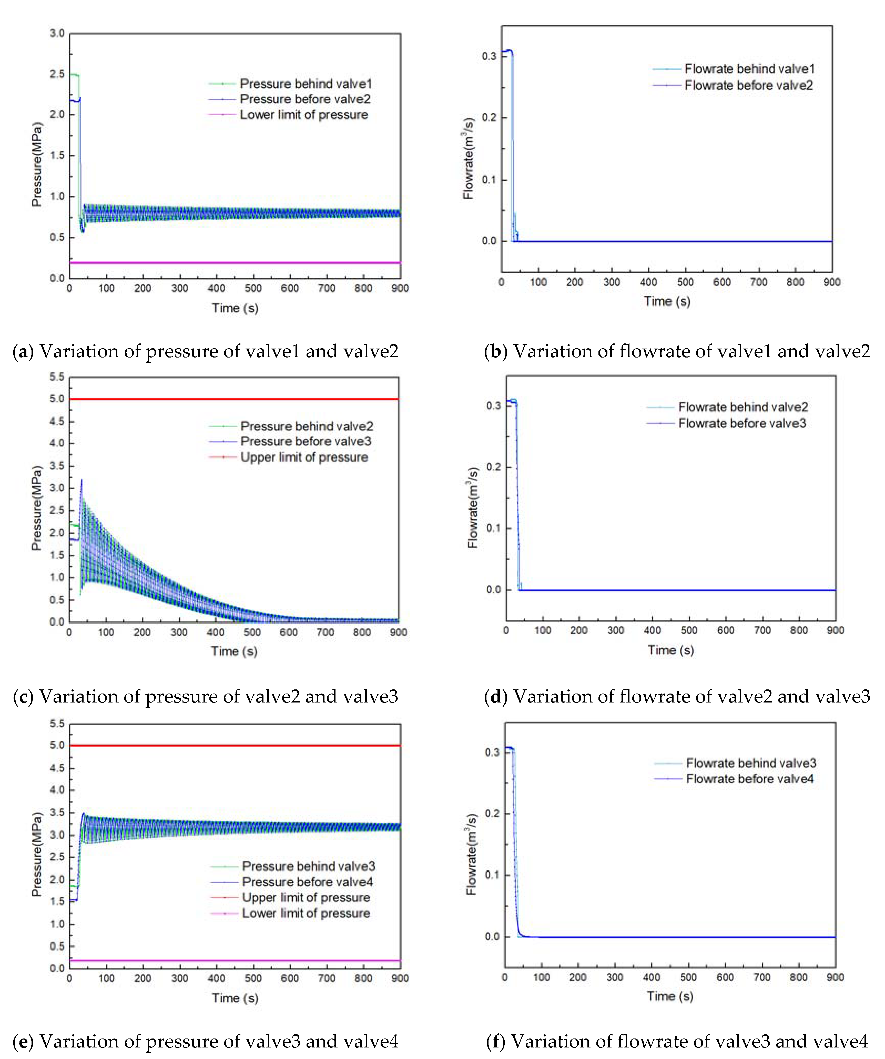
The basic parameter of a liquid pipeline adopted for test is presented in Table 1 and Figure 1.
An actual pipeline is used to verify this model. The pipeline is composed of a pump, four valves and a tank. The pipeline is divided into four equal sections by the pump station and four valves. The pump outlet pressure head is 30 m, and the oil tank inlet pressure head is 20 m, except for valve 4, and the other valves are fully open. The leakage position is in the middle of valve 2 and valve 3. The whole simulation process is 900 s, and leakage occurs at 10 s. At 20 s, the staff stops the pump and closes the valve in sequence.
Under the premise that the water hammer pressure caused by closing the valve is less than the maximum operating pressure of the pipeline, the valves at both ends of the leaking pipeline section should be closed as soon as possible. It is necessary to optimize the opening variation of each valve during the closing process. The optimal results of valve closure under different working conditions are presented as follows.

5.2. Model Test

The valve control scheme is supposed to close each valve along the pipeline sequentially. In Figure 2, the dotted lines indicate the opening variation of each valve, and the solid lines indicate the opening variation with the fastest closure rate. The closure rate of valve 4 is always close to the fastest closure rate because its initial opening is the smallest compared to other valves and its closure time is the shortest. Small water hammer waves generated during valve closing do not cause any overpressure in the pipeline. During the closing of valves 1, 2 and 3, the closure rate changes drastically, especially when it is almost closed. The closure rate is reduced because the water hammer waves caused by valve closing and pump stop are now overlapping, which may cause overpressure in the pipeline. From this point of view, reducing the closure rate can relieve the water hammer pressure and avoid any overpressure. The closure time of each valve along the pipeline is shown in Table 2.
Figure 3 shows the variation of the cumulative leakage volume. As can be seen from the figure, the leakage is basically constant after 650 s, indicating that the pipeline stop leaking. The slope of the curve from 0 to 650 s gradually decreases, indicating that pressure and flow rate of the leakage section are reduced after the leakage control scheme is implemented. In order to ensure the accuracy of this model, the results are compared with the simulation results of SPS whose leakage volume curve is close to the model.
Figure 4 shows the change in pressure and flow at the point of leakage. Figure 4a shows that the pressure at the leak point gradually oscillates and decreases, tending to zero at 650 s. The pressure of the entire valve closure process is less than maximum pressure of the pipeline. Figure 4b shows the change in flow in the pipeline before and after the leak. Positive flow represents the flow from valve 1 to valve 4, and negative flow indicates the opposite direction. The flow periodically oscillates and gradually decreases, becoming zero at 650 s. The steady value of pressure and flow indicates that the leak stops at 650 s, and the result is consistent with Figure 3.
Figure 5 shows the variation of pressure and flowrate at the main nodes of the study pipeline. Figure 5a,b are the curves of pressure and flowrate between the outlet of valve 1 and the inlet of valve 2. It is shown that the pressure of the pipeline section also displays a significant decline after the pump stop at the initial station results in a negative pressure wave spreading through this pipeline section. Then the pressure fluctuates periodically and gradually reduces to a stable value that is higher than the lower limit of pressure and avoids liquid vaporization. Figure 5c,d are the curves of pressure and flowrate between the outlet of valve 2 and the inlet of valve 3, and for a detailed analysis one can refer to Figure 4. Figure 5e,f are the curves of the pressure and flowrate between the outlet of valve 3 and the inlet of valve 4. As the figures show, the pressure in the pipeline increases since the closing valve leads to a boost wave and then the pressure fluctuates periodically and gradually stabilizes within the pressure limits.

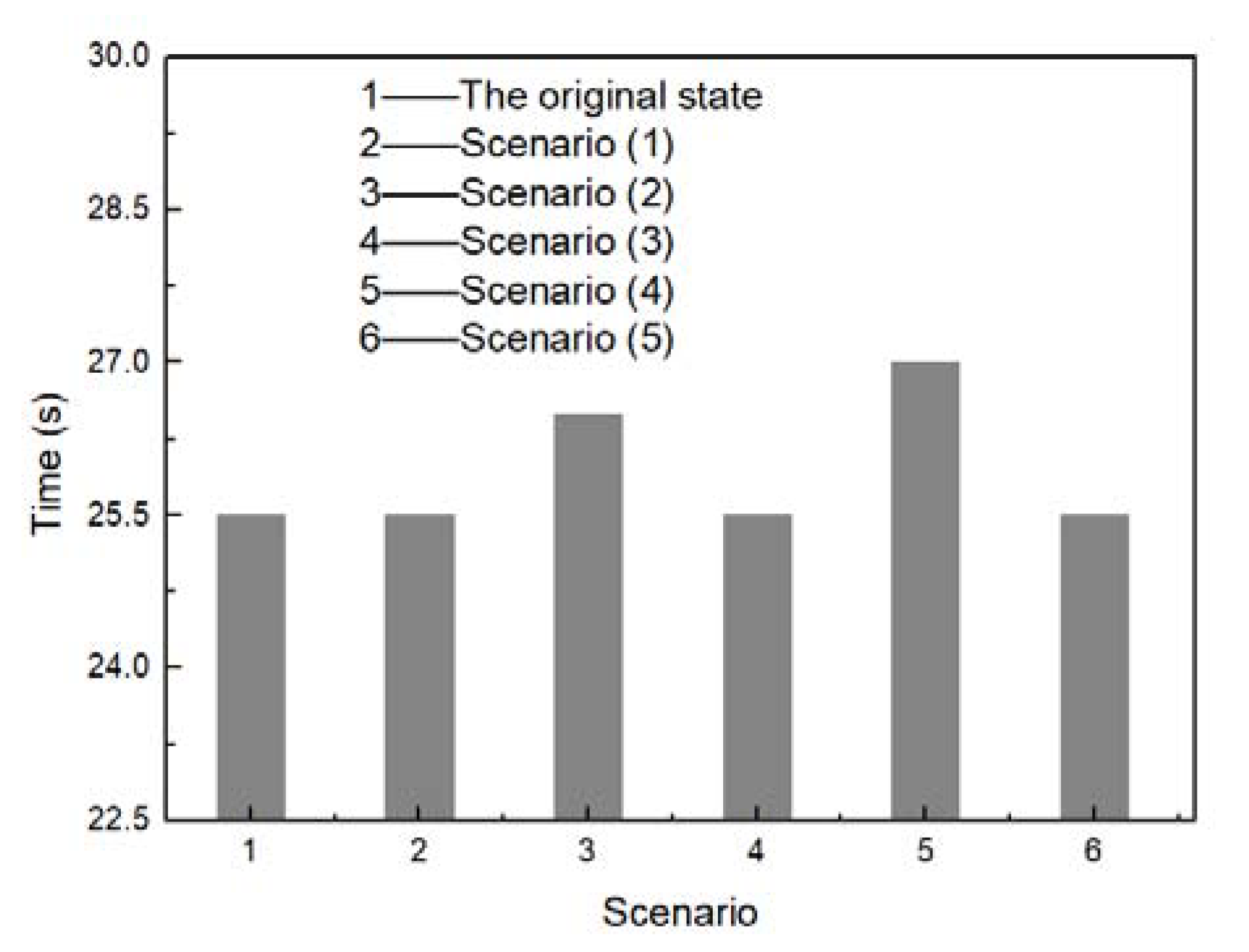
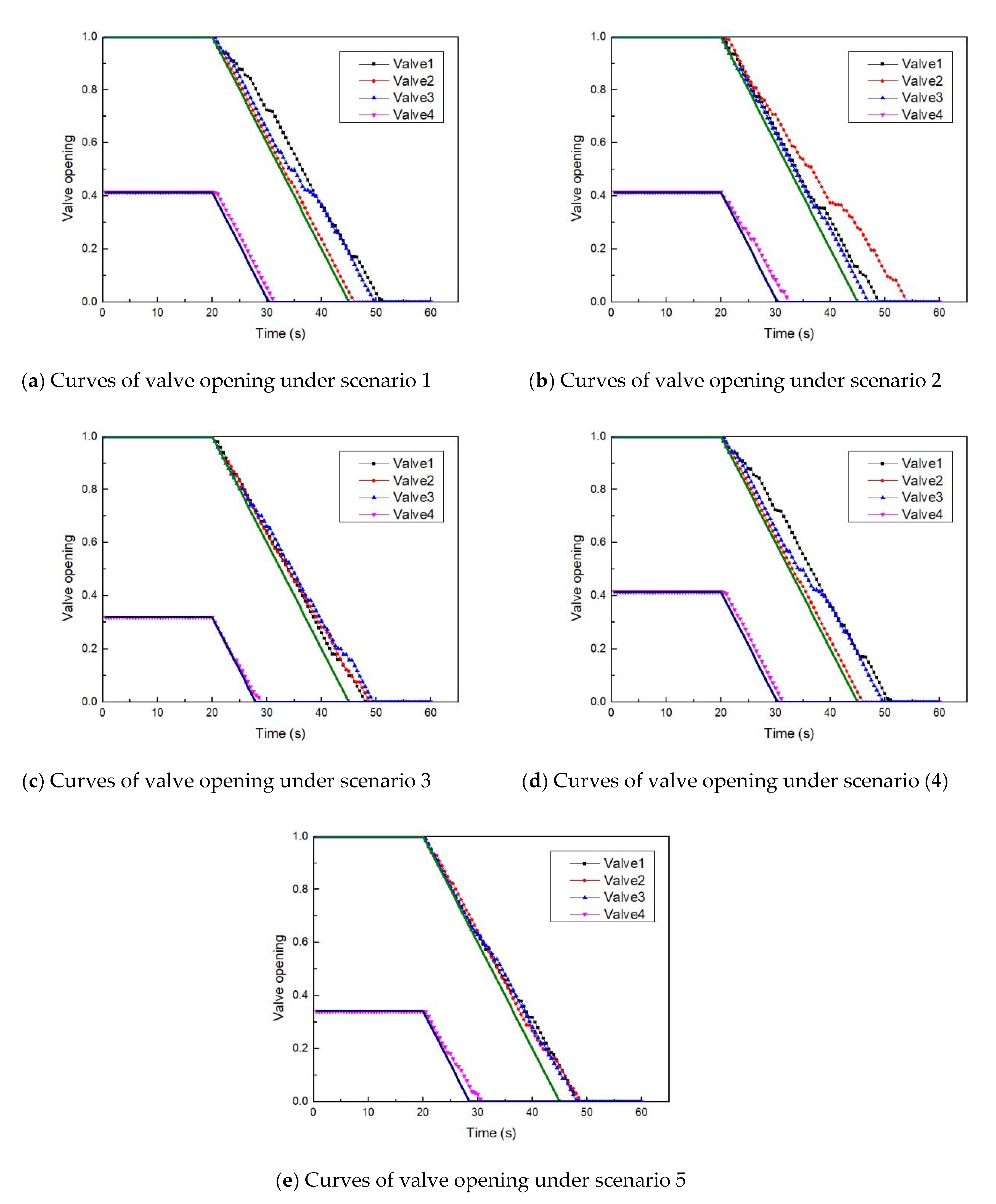
5.3. Exploration for Model Influence Factors

To analyze the factors influencing the valve closure process, the model parameters should be changed to perform the corresponding simulation under the original leak state of the pipeline. There are five scenarios:
Scenario (1): Compared with the original state, the leak position at 12.5 km upstream is substituted by 14 km, but the leak point and the original leak position belong to the same pipeline section.
Scenario (2): Compared with the original state, the leak position at 12.5 km upstream is substituted by 17.5 km, and the leak point and the original leak position belong to different pipeline sections.
Scenario (3): Compared with the original state, we vary the leak coefficient by enlarging the area of the leak aperture, converting it from 0.00008 to 0.0004.
Scenario (4): Compared with the original state, we rise the pressure along the pipeline with an increment of 0.5 MPa for each node.
Scenario (5): Compared with the original state, we reduce the pressure along the pipeline with an increment of 0.5 MPa for each node.
The simulation result and analysis are shown as below. Table 3 presents the comparison among closure time of valves under different simulation scenarios. Figure 6 shows the closure time of valve 2 under the above five scenarios, as well as the comparison with the original state. As seen in the figure, under scenarios (1), (3) and (5), the closure time of valve 2 is similar to the original state. In other words, there will be less influence on valve closure when changing the leak position (the same pipeline section), leak coefficient and the pressure along the pipeline is declining. Under scenarios (2) and (4), the closure time of both valves is prolonged compared with the original state, which means there will be an influence on valve closing when changing the leak position (different pipeline sections) and enhancing the pressure along the pipeline.
Figure 7 shows the closure process of valves under the above five scenarios, where the blue and green curves with no markers indicate the opening variation during the fastest process of valve closing and the slope indicates the fastest closing rate of valves. In the figure, under scenarios (1), (3) and (5), although the rate fluctuates during the whole closure process, it can maintain a higher value. Under scenarios (2) and (4), the curves vary from steep to slow during the whole closure process, and the rate decreases gradually.
Combined with the interpretation for Figure 5 in Section 5.2, it is known that in scenario (2) after the leak point is altered, the pressure in the leak pipeline section is increased, which is similar to scenario (4). It can be deduced that pressure increase will affect valve closing since water hammer results in a pressure increase in the pipeline, which is prone to overpressure, especially when the pipeline is under higher pressure. Therefore, for the healthy operation of pipelines, valves should be closed gradually during valve closing.

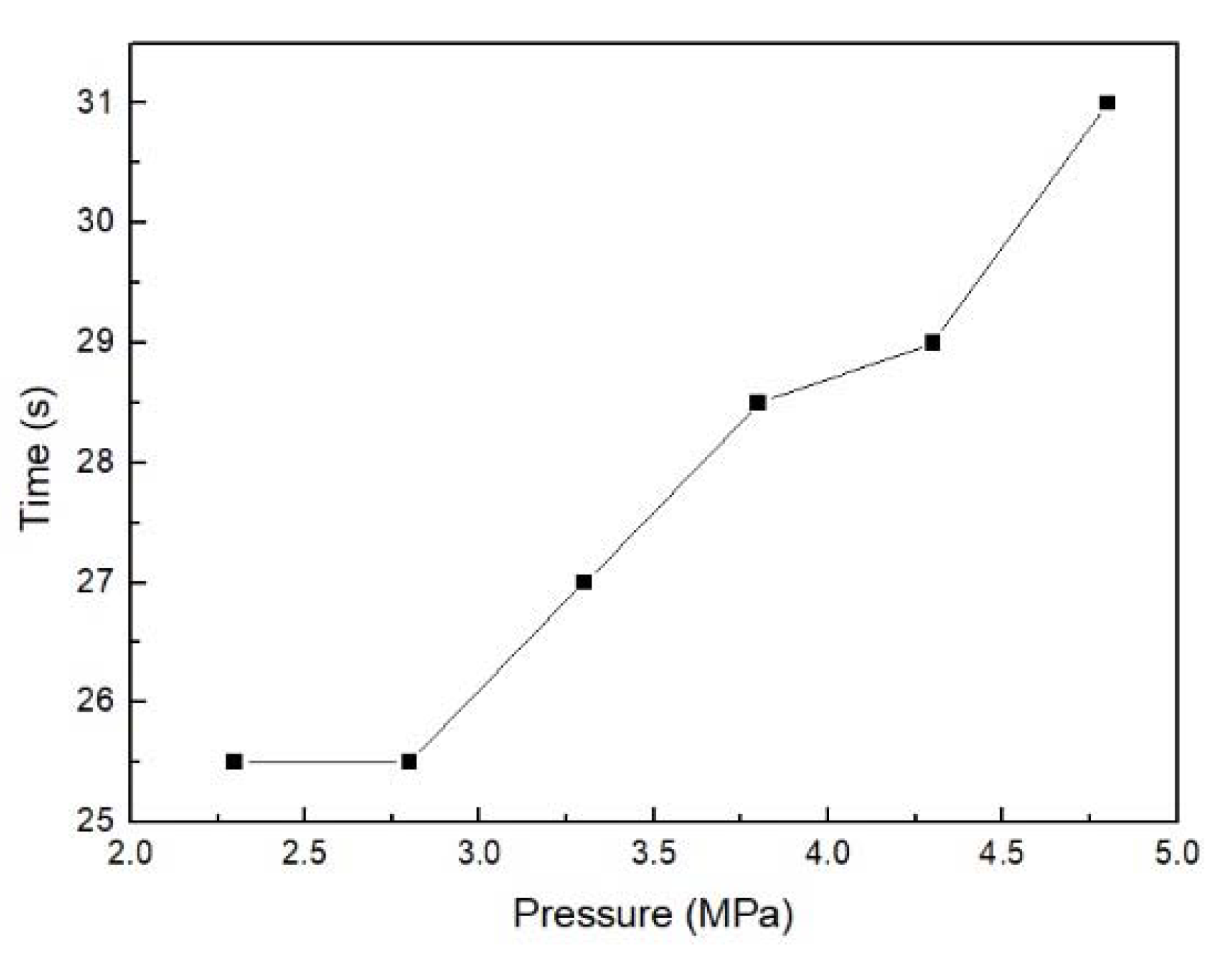
5.4. Analysis on Model Influence Factors

As known from the analysis in Section 5.3, the pressure along the pipeline would affect valve closure. The pressure increase contributes to the increase of the closure time of valves. During the closure process, the rate will gradually slow down in case of overpressure. Thus, this influence factor will be tested next.
The outlet pressure of pumps is perceived as a standard for grade division of the pressure along the pipeline. The outlet pressure improvement of pumps contributes to the pressure improvement along the pipeline. The pressure along the tested pipeline falls into six grades: 2.3, 2.8, 3.3, 3.8, 4.3 and 4.8 MPa.
Figure 8 shows the relationship between the closure time of valve 2 and the pressure along the pipeline. The closure time of valve 2 tends to rise up along with the pressure increase along the pipeline, but when the pressure is smaller, the closure time varies slowly since the valve can be closed in the allowable fastest closure rate to avoid overpressure conditions. Along with the pressure increase along the pipeline, the closure curves of valves change slowly in order to reduce water hammer wave. The closure process and time of each valve under different pipe pressures are presented in Figure 9and Table 4.
Meanwhile, the closure time of scenario (2) is less than that of scenario (4) because the pressure in the changed pipeline section improves due to valve closure, but is still lower than the magnitude of the improvement along the pipeline, therefore, less time is required.
In conclusion, with respect to a real pipeline, simulations in advance can figure out the closure process of valves under different pressure. When a leak happens, executing the closure scheme for valves can correspondingly close valves as soon as possible and simultaneously avoid overpressure.

6. Conclusions

Pipeline leakage hazards can be minimized to a large extent by active control. However, under the leakage conditions, the hydraulic system of the pipeline is quite complicated, and it is difficult to formulate an optimal control scheme of the pipeline hydraulic devices. Since the constraints involve non-linear terms, the current solution algorithms and solvers cannot guarantee a global optimal solution for the non-linear model, therefore, the piecewise linearization method is used to transform the model into MILP, and the model is solved by branch and bound algorithm.
The optimal control on the closed operation for valves under pipeline system leak conditions can be simulated by this model. The closure process and time of valves can be determined to minimize leakage volume as well as water hammer waves. This paper focuses on the closure processes of valves for leaking pipelines under various leak states and pipeline pressures. The following conclusions are given:
(1)
When pipeline sections leak, the opening of each valve along pipeline systems declines at the fastest feasible closure rate. In this way, the shortest closure time of valves can be obtained, leading to the least leakage volume.
(2)
Locating the leak point in different pipeline sections affects the valve control scheme and closure time. When the original states are different or the distance between the leakage point and the start becomes longer, the closure time will be prolonged.
(3)
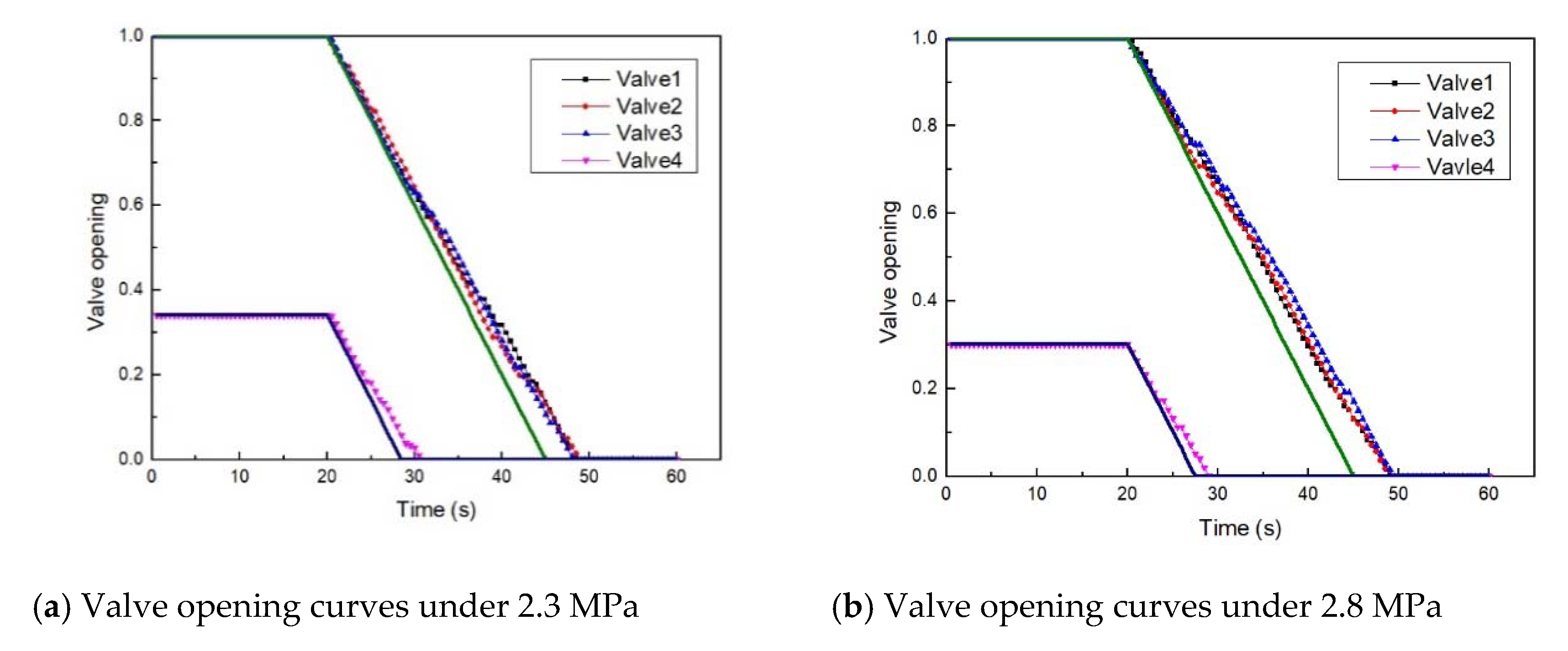
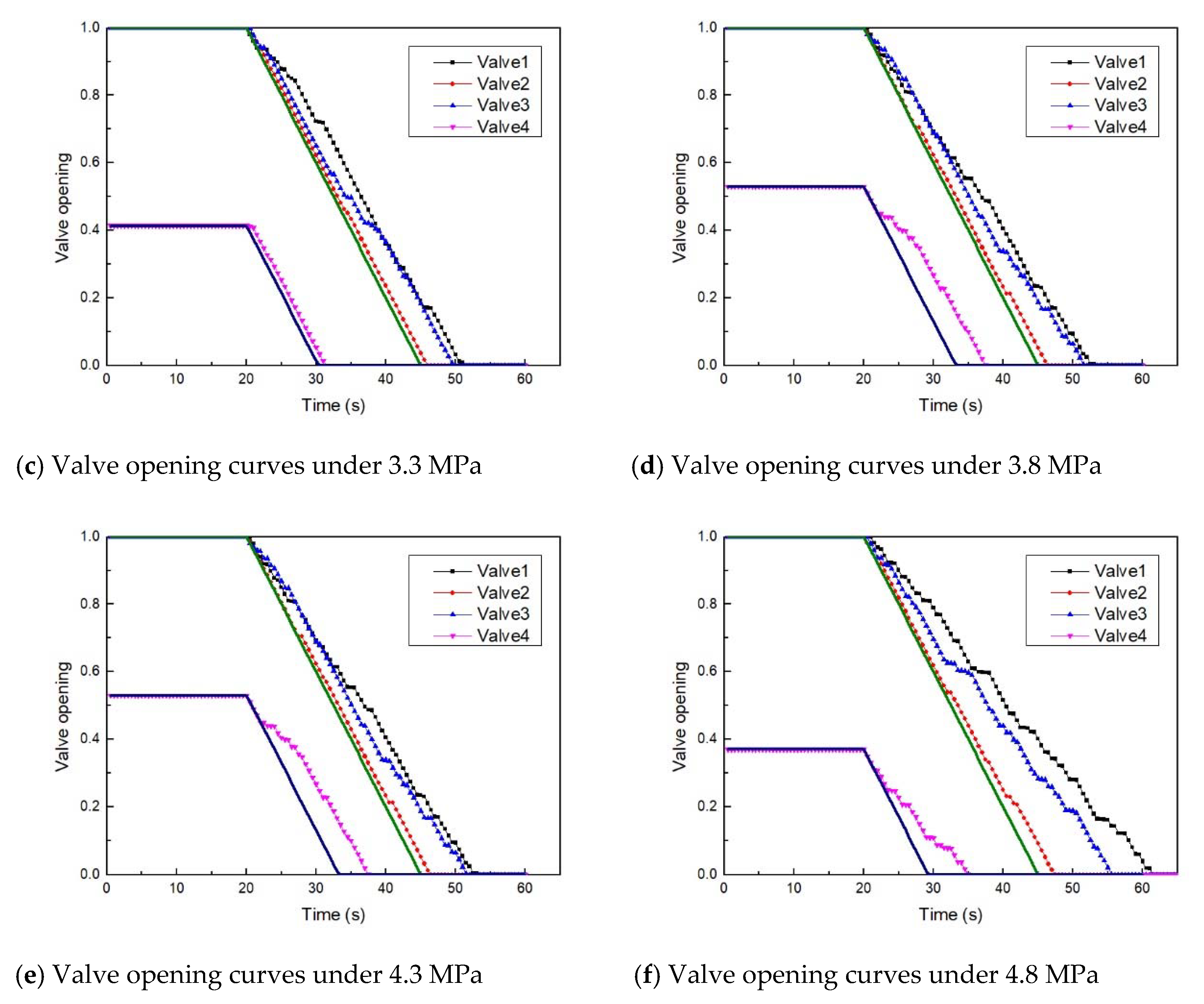
The pressure in pipelines affects the closure time and scheme of valves. As the pressure increases along the pipeline, the closure time before the leak point tends to rise and a lower pressure will contribute to less closure time fluctuation because at this moment, valves will be closed at the fastest allowable closure rate and overpressure will not happen.
In summary, the model proposed in this paper is capable of figuring out the closure process and time of valves under various pipeline states by simulating different pipeline leakage conditions in advance, consequently helping plan a closure scheme for different valves. When leakage occurs, the fastest valve closure and normal pressure fluctuations can be achieved by executing the corresponding closure scheme.

Author Contributions

Methodology, W.Z. and H.Z.; Supervision, Y.L.; Writing—original draft, W.Z.; Investigation and data curation, N.X.; Writing—review & editing, R.S. All authors have read and agreed to the published version of the manuscript.

Funding

This research was funded by the National Natural Science Foundation of China, grant number: 51874325.

Acknowledgments

This work was partially supported by the National Natural Science Foundation of China (“Study on Optimization and Supply-side Reliability of Oil Product Supply Chain Logistics System”, No. 51874325). The authors are grateful to all study participants.

Conflicts of Interest

The authors declare no conflicts of interest.

Nomenclature

Symbols
aVelocity of pressure wave in the pipeline (m/s)
ALThe area of leak aperture (m2)
B s j Binary variable of cut-off valves
B A i , a j Binary variable of distinguishing flowrate ranges
CdOrifice flow coefficient, 0.98–0.99, dimensionless
CvLeak coefficient, Cv = AL·Cd·α, dimensionless
DThe inner diameter of the pipeline (m)
EModulus of elasticity (Pa)
fFrictional coefficient along the pipeline, dimensionless
gGravitational acceleration (m/s2)
HHydraulic head in pipeline (m)
H i j Hydraulic head of pipeline section i at moment j (m)
HLInner hydraulic head at leak point (m)
HeHydraulic head outside leak aperture (m)
HViActual measuring hydraulic head of pipeline section i (m)
KBulk modulus of elasticity (Pa)
LPipeline length (km)
mCoefficient associated with flow regime
MPenalty coefficient
PmaxiUpper limit of pipeline pressure (Pa)
Q i j Cross-section flowrate of pipeline section i at moment j (m3/h)
Q i j m Flowrate of pipeline section i at end moment (m3/h)
Q i s j Flowrate of pipeline start at moment j (m3/h)
Q L j Flowrate of the leak aperture which is L from pipeline start at moment j (m3/h)
QmaxaMaximum flowrate in flowrate range a (m3/h)
QminaMinimum flowrate in flowrate range a (m3/h)
ΔtClosure time of valves (s)
xDistance of leak point from the upstream station (m)
vAverage flow velocity of the fluid in the pipeline (m/s)
Greek symbols
αFlow contraction coefficient, 0.62–0.66, dimensionless
αaConstant item coefficient of pipeline flowrate linearization in flowrate range a
ρaVariable coefficient of pipeline flowrate linearization in flowrate range a
υaConstant item coefficient of the linearization flowrate at leak aperture in flowrate range a
ωaVariable coefficient of the linearization flowrate at leak aperure in flowrate range a
ρAverage density of the fluid in the cross-sectional area (kg/m3)
ψ i j iClosure rate of upstream valves of pipeline section i at j moment
ψisOpening of valves locating at upstream leak pipeline section
ψiOpening of cut-off valves at end moment
ΔϕmaxUpper limit of closed rate of valves

References

  1. Hou, P.; Yi, X.; Dong, H. A Spatial Statistic Based Risk Assessment Approach to Prioritize the Pipeline Inspection of the Pipeline Network. Energies 2020, 13, 685. [Google Scholar] [CrossRef] [Green Version]
  2. Ramírez-Camacho, J.G.; Carbone, F.; Pastor, E.; Bubbico, R.; Casal, J. Assessing the consequences of pipeline accidents to support land-use planning. Saf. Sci. 2017, 97, 34–42. [Google Scholar] [CrossRef]
  3. Inanloo, B.; Tansel, B.; Shams, K.; Jin, X.; Gan, A. A decision aid GIS-based risk assessment and vulnerability analysis approach for transportation and pipeline networks. Saf. Sci. 2016, 84, 57–66. [Google Scholar] [CrossRef]
  4. Alkhaledi, K.; Alrushaid, S.; Almansouri, J.; Alrashed, A. Using fault tree analysis in the Al-Ahmadi town gas leak incidents. Saf. Sci. 2015, 79, 184–192. [Google Scholar] [CrossRef]
  5. Reddy, H.P.; Narasimhan, S.; Bhallamudi, S.M.; Bairagi, S. Leak detection in gas pipeline networks using an efficient state estimator. Part-I: Theory and simulations. Comput. Chem. Eng. 2011, 35, 651–661. [Google Scholar] [CrossRef]
  6. Wang, F.; Lin, W.; Liu, Z.; Qiu, X. Pipeline Leak Detection and Location Based on Model-Free Isolation of Abnormal Acoustic Signals. Energies 2019, 12, 3172. [Google Scholar] [CrossRef] [Green Version]
  7. Mandal, S.K.; Chan, F.T.; Tiwari, M.K. Leak detection of pipeline: An integrated approach of rough set theory and artificial bee colony trained SVM. Expert Syst. Appl. 2012, 39, 3071–3080. [Google Scholar] [CrossRef]
  8. Liang, W.; Zhang, L.-B. A wave change analysis (WCA) method for pipeline leak detection using Gaussian mixture model. J. Loss Prev. Process. Ind. 2012, 25, 60–69. [Google Scholar] [CrossRef]
  9. Vankov, Y.; Rumyantsev, A.; Ziganshin, S.; Politova, T.; Minyazev, R.; Zagretdinov, A. Assessment of the Condition of Pipelines Using Convolutional Neural Networks. Energies 2020, 13, 618. [Google Scholar] [CrossRef] [Green Version]
  10. Elaoud, S.; Hadj-Taïeb, L.; Hadj-Taieb, E. Leak detection of hydrogen–natural gas mixtures in pipes using the characteristics method of specified time intervals. J. Loss Prev. Process. Ind. 2010, 23, 637–645. [Google Scholar] [CrossRef]
  11. Hermansyah, H.; Hidayat, M.N.; Kumaraningrum, A.R.; Yohda, M.; Shariff, A.M. Assessment, Mitigation, and Control of Potential Gas Leakage in Existing Buildings Not Designed for Gas Installation in Indonesia. Energies 2018, 11, 2970. [Google Scholar] [CrossRef] [Green Version]
  12. Meng, L.; Yuxing, L.; Wuchang, W.; Juntao, F. Experimental study on leak detection and location for gas pipeline based on acoustic method. J. Loss Prev. Process. Ind. 2012, 25, 90–102. [Google Scholar] [CrossRef]
  13. Liu, Z.; Zhou, Y.; Huang, P.; Sun, R.; Wang, S.; Xiaohong, M.A. Scaled field test for COleakage and dispersion from pipelines. Ciesc J. 2012. [Google Scholar]
  14. Xie, Q.; Tu, R.; Jiang, X.; Li, K.; Zhou, X. The leakage behavior of supercritical CO2 flow in an experimental pipeline system. Appl. Energy 2014, 130, 574–580. [Google Scholar] [CrossRef]
  15. Koornneef, J.; Spruijt, M.; Molag, M.; Ramirez, A.; Turkenburg, W.; Faaij, A. Quantitative risk assessment of CO2 transport by pipelines—A review of uncertainties and their impacts. J. Hazard. Mater. 2010, 177, 12–27. [Google Scholar] [CrossRef]
  16. Cleaver, R.; Cumber, P.; Halford, A. Modelling outflow from a ruptured pipeline transporting compressed volatile liquids. J. Loss Prev. Process. Ind. 2003, 16, 533–543. [Google Scholar] [CrossRef]
  17. Mahgerefteh, H.; Oke, A.O.; Rykov, Y. Efficient numerical solution for highly transient flows. Chem. Eng. Sci. 2006, 61, 5049–5056. [Google Scholar] [CrossRef]
  18. Choi, J.; Hur, N.; Kang, S.; Lee, E.D.; Lee, K.B. A CFD simulation of hydrogen dispersion for the hydrogen leakage from a fuel cell vehicle in an underground parking garage. Int. J. Hydrog. Energy 2013, 38, 8084–8091. [Google Scholar] [CrossRef]
  19. He, X.; Zhang, Y.; Wang, C.; Zhang, C.; Cheng, L.; Chen, K.; Hu, B. Influence of Critical Wall Roughness on the Performance of Double-Channel Sewage Pump. Energies 2020, 13, 464. [Google Scholar] [CrossRef] [Green Version]
  20. Gorenz, P.; Herzog, N.; Egbers, C. Investigation of CO 2 Release Pressures in Pipeline Cracks. Energy Procedia 2013, 40, 285–293. [Google Scholar] [CrossRef] [Green Version]
  21. Molag, M.; Dam, C. Modelling of accidental releases from a high pressure CO2 pipelines. Energy Procedia 2011, 4, 2301–2307. [Google Scholar] [CrossRef] [Green Version]
  22. Mazzoldi, A.; Hill, T.; Colls, J.J. CFD and Gaussian atmospheric dispersion models: A comparison for leak from carbon dioxide transportation and storage facilities. Atmos. Environ. 2008, 42, 8046–8054. [Google Scholar] [CrossRef]
  23. Zhang, H.; Zhang, W.; Xu, N.; Yuan, M.; Liang, Y. Control optimization for liquid pipelines under leak condition. In Proceedings of the 2018 7th International Conference on Industrial Technology and Management (ICITM), Oxford, UK, 7–9 March 2018; pp. 42–46. [Google Scholar]
  24. Plapp, J.E. Engineering Fluid Mechanics. Available online: https://www.springer.com/gp/book/9781402067419 (accessed on 20 January 2020).
Figure 1. Hydraulic system of pipeline.
Energies 13 01692 g001
Figure 2. Variation of valve opening with time.
Energies 13 01692 g002
Figure 3. Variation of accumulative leakage with time.
Energies 13 01692 g003
Figure 4. Variation of pressure and flowrate at the leak point.
Energies 13 01692 g004
Figure 5. Variation of pressure and flowrate at main point.
Energies 13 01692 g005
Figure 6. Closure times of Valve 2 under different scenarios.
Energies 13 01692 g006
Figure 7. Curves of valve opening under different scenarios.
Energies 13 01692 g007
Figure 8. Closure time of valve 2 under different pressure grades.
Energies 13 01692 g008
Figure 9. Valve opening curves under different pressure grades.
Energies 13 01692 g009aEnergies 13 01692 g009b
Table 1. Pipeline parameters.
Pipe Length L/kmPipe Specification D × Φ/mm × mmModulus of Elasticity E/PaLeak Coefficient CvLeak Position X/km
20457 × 7.1207 × 1090.0000812.5
Fluid Density ρ /kg·m−3Fluid Viscosity ν /m2·s−1Bulk Modulus of Elasticity K/PaPump Characteristic Parameters A Pump Characteristic Parameters B
8307.02 × 10−61.39 × 109392.85807.6
Table 2. Closed times of valves under original state.
No.Valve1Valve 2Valve 3Valve 4
Time/s33.025.531.517.5
Table 3. Comparison among closed time of valves under different simulation scenarios.
ScenarioTime/s
Valve 1Valve 2Valve 3Valve 4
Original state33.025.531.517.5
Scenario (1)31.025.529.511.0
Scenario (2)28.526.534.012.0
Scenario (3) 30.525.534.011.0
Scenario (4)41.027.035.515.0
Scenario (5)27.525.528.515.5
Table 4. The closed time of valves under different pressure grades.
Pressure Grades/MPaTime/s
Valve 1Valve 2Valve 3Valve 4
2.327.525.528.515.5
2.833.025.531.517.5
3.341.027.035.515.0
3.828.528.528.010.5
4.328.529.028.58.5
4.830.031.031.011.0

