Article

Effect of the Intake Valve Lift and Closing Angle on Part Load Efficiency of a Spark Ignition Engine

Automotive Powertrain Technologies Laboratory, Empa Swiss Federal Laboratories for Materials Science and Technology, 8600 Dübendorf, Switzerland
*
Author to whom correspondence should be addressed.
Energies 2020, 13(7), 1682; https://doi.org/10.3390/en13071682
Submission received: 11 February 2020 / Revised: 12 March 2020 / Accepted: 20 March 2020 / Published: 3 April 2020
(This article belongs to the Special Issue Advances in Spark-Ignition Engines)

Abstract

:
This study provides an experimental evaluation of the effectiveness of Miller cycles with various combinations of lift and intake valve closing angle for a passenger car engine with premixed combustion in naturally aspirated operation. A fully variable electro-hydraulic valve train provided different valve lift profiles. Six load points, from 1.5 up to 5 bar brake mean effective pressure at a constant engine speed of 2000 min−1, were tested with 6 different intake valve lift/intake valve closing angle combinations. The intake valve closing angle was always set before bottom dead center to achieve the desired load with unthrottled operations. Experimental comparison with throttled operation outlines an indicated efficiency increase of up to 10% using high intake lift with early valve closing angle. Furthermore, this analysis outlines the influences that early intake valve closing angle has on fuel energy disposition. Longer combustion duration occurs using early intake valve closing angle because of turbulence dissipation effects, leading to slight reductions in the heat-to-work efficiency. However, overall pressure and temperature levels decrease and consequently heat losses and losses due to incomplete combustion decrease as well. Overall, we found that combustion deterioration is compensated/mitigated by the reduction of the heat losses so that reductions of pumping losses using early intake valve closing can be fully exploited to increase the engine’s efficiency.

1. Introduction

This work outlines an experimental investigation of unthrottled Miller cycles using a self-developed electro hydraulic valve train [1,2]. While valve lift is set for all cylinders on the intake and exhaust side, respectively, the valve timing is set individually for the intake- and exhaust valves for each cylinder.
In conventional stoichiometrically operated spark ignition engines, which control the amount of aspirated gas by throttling the intake airflow, pumping losses make the engine efficiency deteriorate significantly, in particular at low loads. This leads to high fuel consumption during typical operation of non-hybrid powertrains [3]. Controlling the amount of fresh gas by adjusting the intake valve closing (IVC) angle promises to reduce or eliminate pumping losses. The intake valves can be closed either before or after bottom dead center. The resulting cycles are usually called Miller and Atkinson, respectively. Late IVC (Atkinson) as a general strategy for load control is problematic, because late intake closing interferes at low load with the ignition angle. Therefore, early IVC (Miller) was used throughout the work presented here.
Whether avoiding pumping losses by early IVC in a spark-ignited concept increases the engine’s brake efficiency or not is, however, not clear a priori because of the following detrimental effects:
1. Miller cycles are normally used to increase the efficiency and are characterized by a larger expansion ratio compared to the compression ratio [4]. To maintain an effective compression ratio, the geometrical compression ratio is increased. However, load control by phasing the IVC while keeping the geometrical compression ratio reduces the effective compression ratio with decreasing load.
2. Although Miller timing reduces pumping losses, it also reduces turbulence intensity. Turbulent kinetic energy is generated during the intake flow process and dissipated later because no momentum addition is present to compensate for the viscous losses [5]. The fast turbulence dissipation for the same engine as used in this research with its standard valve timing settings, but with direct gas injection, is documented in [6]. The earlier the valve closes, the lower the turbulence present during combustion therefore is, which leads to a lower turbulent flame speed. Using early intake closing, the combustion is expected to be slower and less efficient [7].
Miller cycles are often achieved using camshaft-based systems, limiting the possible advantages. A paper by Unger and Schwartz [8] lists the progress and challenges of unthrottled Miller cycles achieved with a serial-production continuously variable valve train where valve timing it strongly coupled to the valve lift. As a result, at low load operating points the maximum valve lift is even lower than 1 mm [9]. This leads unavoidably to strong throttling effects for short valve openings, mainly because the valve’s opening and closing velocities become very low. This drawback does not exist for the electro hydraulic valve train used here, as the valve movement (i.e., the time from fully closed to fully open and vice versa) is independent from valve lift or valve timing.
Therefore, the work presented here allows experimental quantification of the net effects of early intake valve closing and valve lift to the engine’s efficiency independently. The analysis also focuses on the identification and quantification of the individual losses arising from Miller cycles.

2. Experimental Setup

Experiments were performed on a Volkswagen engine with four cylinders and a displacement of 1.4 L, which was operated with port-fuel-injected natural gas and controlled under stoichiometric conditions. The complete camshaft system—composed of the camshaft, gears, chain, and timing adjustment—was removed and the engine was fitted with the electro hydraulic valve train (shown in Figure 1, left).
The cylinder head was modified to hold the variable valve system, while the entire short block remained unchanged from factory specifications. The entire engine control and valve train control were based on a single dSPACE Microautobox rapid prototyping system and the control functionalities were all fully developed in house. Besides the control of injection, ignition, and valve train, the engine control also recorded the cylinder pressure signals of all cylinders and provided closed-loop control of the center of combustion. The center of combustion, estimated online with the Rassweiler and Withrow method [10], was set to 368 °CA by closed-loop-control of the ignition angle. This value was chosen for all the experiments as it gives the highest efficiency (or maximum brake torque, respectively) and it ensured stable operation [11]. Figure 1 (right) provides a picture of the test-bench setup (engine and entire control unit) and Table 1 lists the main characteristics of the experimental setup.
The working principle of the valve train is basically a hydraulically excited spring–mass-system [12] which is able to recover energy. Because of the nature of a spring-mass–system, its oscillation frequency (hence the opening or closing duration in the time domain) is independent in the amplitude (hence the valve lift). The oscillation frequency is set, for a given mass of the moving parts, by choosing the stiffness of the springs. This is done in such a way that an adequate valve opening duration is achieved at the engine’s maximum speed. In the current setup, a duration for valve opening of around 3 ms was chosen. Constant opening and closing durations in the time domain translate to the faster movements in the crank angle domain as the engine speed was reduced. This lead to a very fast release or blocking of the gas flow at lower engine speed.
On the intake side, the valve lifts were set by the hydraulic pressure level. The opening of the valves was initiated by energizing a magnetic coil [13]. The valves remained open until the current to the coil was cut. The valve lift profiles are divided into three main phases: opening, holding and closing. All three phases were mechanically automated to allow opening, keeping open, closing, recuperation of hydraulic fluid and soft seating without the need of electronical feedback control of the valve lift and with just one magnetic coil per actuator [1]. Because of the efficient recuperation, the energy demand of the electro hydraulic valve train was lower than that of cam-driven valve systems.
Figure 2 shows a scheme of the test-bench and depicts the relevant signals (Data acquisition, control units and main mechanical parts).
Figure 3 shows intake valve lift measurements at an engine speed of 2000 min−1 recorded during the fired engine experiments explained in detail in the following sections. These experiments were performed in order to characterize different Miller cycles, as well as the influence that different combinations of IVC time and lift have on pumping losses variation and efficiency. For the sake of consistency, all the valve timings except IVC angle and intake lift were kept constant for all experiments. As Figure 3 shows, the time to open or close the valves remained constant, independent of the valve lift, which ensures a fast release of the flow area even at low valve lifts. This fast opening, even for small valve lifts, is a major advantage of the system described here.
The intake valve lift was measured for each cylinder using the linear encoder (reported in Table 1) and it depended only on the hydraulic pressure level, which is the control input. For the sake of simplicity, only the maximum achieved lift for each pressure level was used throughout this analysis.

3. Theoretical Considerations and Description of Procedures

The mass flow ( m ˙ ) through the intake valve can be described using an approximated form of the isenthalpic orifice equation for compressible fluids, as reported in Appendix A. The approximation was used to qualitatively describe the flow through the intake valve. When the effective area is small ( c d A ), namely at low lifts, the mass flow decreases, hence lowering the in cylinder pressure during the aspiration phase and increasing the pumping losses [14]. The valve throttling effect is less significant at lower piston speeds, which occur around top dead center and bottom dead center, and generally at lower engine speeds.
Intake valve opening time, exhaust valve opening and closing instants, and exhaust valve lift were kept constant during all experiments described here. To compensate for cylinder-to-cylinder distribution and for the small difference between valve profiles during each test, the indicated mean effective pressure (IMEP) was kept constant in all the cylinders by closed-loop-control of IVC timing for each cylinder individually. Since the IMEP was the same in all cylinders, the mass per cylinder was approximated as one fourth of the total mass flow measured. This approximation holds by assuming that the indicated efficiency is the same in all the four cylinders.
A constant load level can be achieved with different combinations of IVC time and intake lift. For similar loads, four concurring influences driving the fuel efficiency were identified:
1. Variation in pumping losses due to different valve lift.
2. Variation in combustion efficiency due to earlier IVC time resulting in slower combustion due to a lower turbulence.
3. Influence due to lower overall pressures and temperatures during the high-pressure loop IMEP using earlier IVC timing.
4. Influence of lowering the compression ratio while keeping the expansion ratio constant.
The burned rate variation was analyzed following the procedure outlined in [15]. With this methodology, the combustion characteristics were evaluated through the mass fraction burned (xB). The calculation procedure is reported in Appendix B. The positive and negative IMEP were calculated from cylinder pressure and volume. The area enclosed by the part of the cycle that runs clockwise (counterclockwise) represents the positive (negative) work. The negative work represents the pumping mean effective pressure (PMEP). In contrast, the 360 degree integration between top dead center and top dead center enables a correct reading in terms of total work, but it provides a false division between positive and negative IMEP [16].
To compare the Miller unthrottled experiments with normal throttled operations, the valve timings were not changed, with exception of IVC, which was set to 200 °CA after top dead center and lift, which was kept at 3.5 mm. The lift was not increased any further because, for the engine speed analyzed, no differences were observed when using higher lifts. To achieve the same load as with IVC variation, the intake manifold pressure was controlled using a throttle.
To evaluate the experimental uncertainty, the measurement uncertainty of the individual sensors has to be taken into account. Table 2 lists the uncertainties for each used measurement (m).
The experimental uncertainty (ΔV) was calculated according to Equation (1), where m indicates the measurement. This calculation assumes the worst-case scenario of linear error propagation.
V i = | V i m i | m i

4. Results and Discussion

In the first step, described in Section 4.1, the experiments were analyzed as a function of IMEP. This was to gain a basic insight about the different influences of early intake valve closing angle and valve lift on overall efficiency, pumping losses, and combustion deterioration. Afterwards, in Section 4.2, a brief comparison between unthrottled and throttled operation is presented. In the third step, in Section 4.3, a Willans analysis was used, as explained in [17], to distinguish between influences on thermodynamic efficiencies and gas exchange losses. Finally, in Section 4.4, the first law energy balance [18] is described for a constant fuel mass flow, different valve timings, and manifold pressures. This analysis provides insights about the disposition of the initial fuel energy [19].
All experiments and analyses were performed at an engine speed of 2000 min−1 for different engine loads. This engine speed is chosen because it represents a typical maximal engine speed during urban driving cycles [20] where pumping losses have a big impact on the efficiency.

4.1. Intake Valve Closing Angle and Lift Combinations (IMEP Analysis)

The same loads were achieved at different valve lifts using different IVC angles. The goal was to reconstruct the influences driving the efficiency variation for different IVC and lift combinations. Thanks to the fast opening of the valves, lifts as low as 0.9 mm were relevant for analysis. Lifts higher than 4.1 mm were not analyzed because, for the chosen engine speed and loads, no effects were seen using higher lifts. 
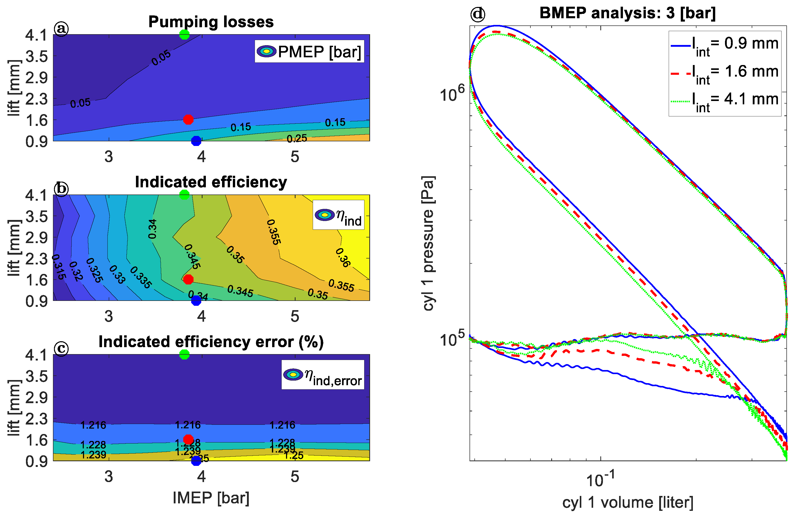
Figure 4 illustrates: (a) the pumping losses; (b) the indicated efficiencies; and (c) the experimental uncertainty of the indicated efficiency as a function of IMEP and intake valve lift. Plot (d) shows the pressure volume diagram of three experiments in double logarithmic scale. The engine output of all three experiments was the same, 3 bar brake mean effective pressure (BMEP), but it was achieved with different IVC and lift combinations. These three experiments are highlighted in the (a), (b) and (c) plots in Figure 4 with blue red and green points. It has to be pointed out that the energy demand for valve actuation depends, among other parameters, on the valve lift. Smaller valve lifts mean less losses for valve actuation, especially because a large part of the actuation energy for exhaust valves is dissipative and cannot be recovered with any valve actuation system. Therefore, choosing the minimum valve lift for best indicated efficiency is generally beneficial.
Pumping losses, plot (a) in Figure 4, considerably decreased at constant IMEP for higher lifts and they slightly increased at constant lift for higher IMEP. For higher lifts, the pressure difference between in cylinder and intake manifold (which is close to ambient pressure with throttle fully open) decreased (by same mass flow), reducing the pumping losses. To achieve the same in cylinder mass, the IVC was therefore advanced. The increase of PMEP at higher loads and constant lift can be explained by the cylinder motion. In fact, the cylinder accelerated from top dead center to maximal speed at half stroke and decelerated in the second half stroke. For this reason, the in-cylinder pressure during intake in the middle of the stroke decreased. For constant valve lift, higher pumping losses occurred at higher loads. Two factors influenced the variation of indicated efficiency, plot (b) in Figure 5. Firstly, the efficiency increased at higher loads. This is a normal trend in internal combustion engines, as some losses (e.g., wall heat losses) do not proportionally scale with load. Additionally, at higher loads, the thermodynamic efficiency increases due to the more efficient combustion. Secondly, the efficiency increased at higher lifts, thanks to the reduction in PMEP. No clear decrease in indicated efficiency was visible at high lifts. In fact, early IVC time could not only be responsible for reduced PMEP, but also for combustion deterioration, and hence lower efficiency due to lack of turbulence. Nevertheless gas exchange improvement at the engine speed of 2000 min−1 investigated here was found to always overcome the possible degradation of the combustion process. The valve train was able to achieve valve lifts up to 9 mm, but for the engine speed of 2000 min−1 discussed here lifts above 4 mm did not show an additional gain. As higher valve lifts need more energy for the valve train itself, which would negatively affect the engine’s effective work, an adaption of the valve lift to the engine speed is beneficial.
The pV diagram, plot (c) in Figure 4, depicts the same loads, achieved with different combinations of IVC angle and lift. The three analyzed experiments are also shown as points in plots (a), (b) and (c) in Figure 5. The important parameters for these experiments are listed in Table 3.
At higher lifts, the IVC timing was advanced to keep the load constant. Earlier IVC corresponds to lower effective compression ratio, lowering the overall pressure during the high pressure loop (shown in Figure 4 plot d). As expected, the pumping losses increased at lower lifts (up to four times). During the gas exchange process (where pumping losses occur), the lines diverged most between 0.1 and 0.3 L (visible in Figure 4 plot d). The pumping losses were mainly present in the middle of the stroke, where the piston moves fastest. Comparing these unthrottled operating points, the fuel consumption was reduced up to 3% (relativ) at 3 bar BMEP with higher lifts and earlier valve closing.
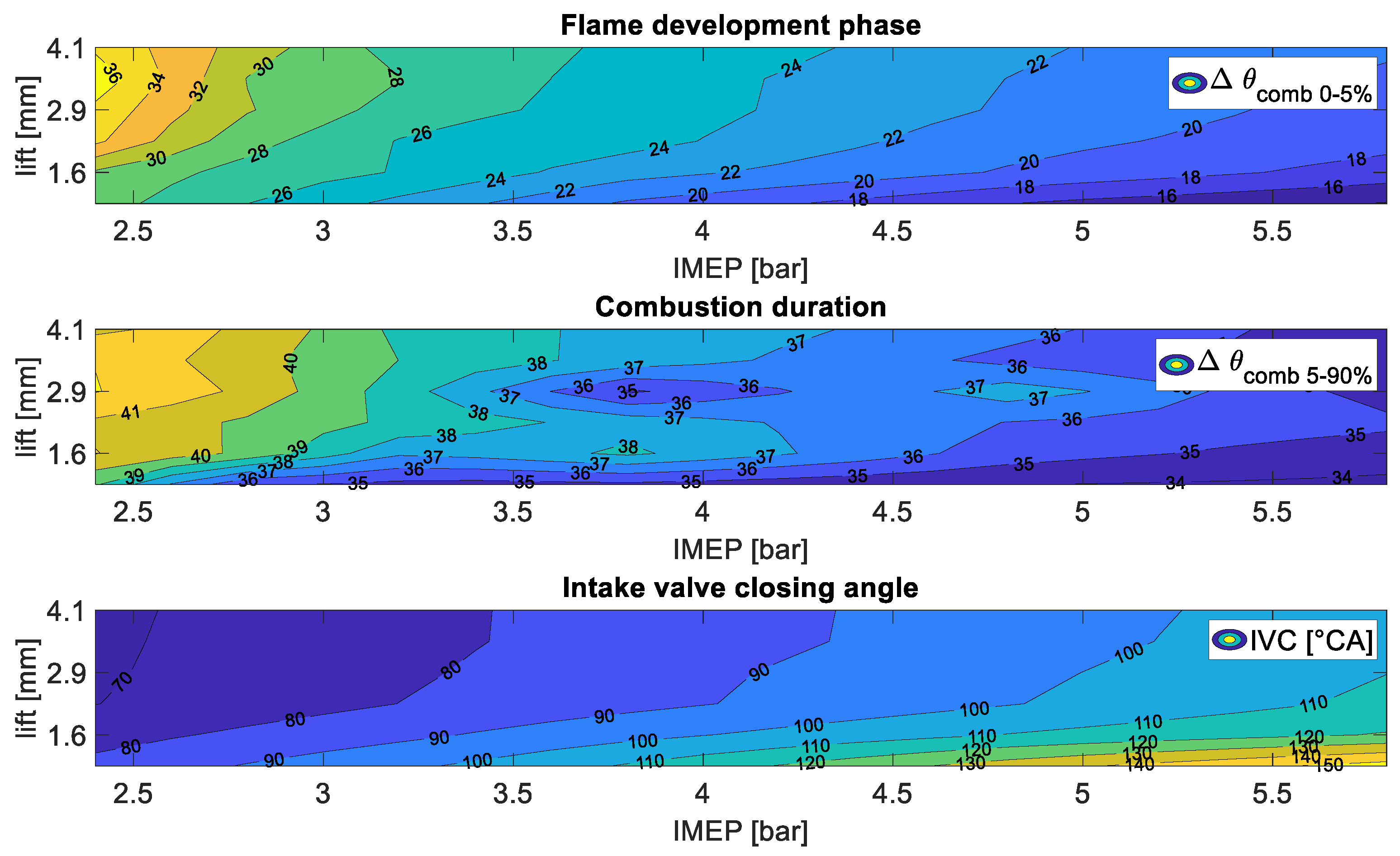
To understand the magnitude of the combustion deterioration, the burned rate variation was analyzed. Figure 5 depicts the flame development phase (0–5% of mass fraction burned), the main combustion duration (5–95% of mass fraction burned), and the IVC angle as a function of IMEP and lift.
The flame development phase and combustion duration show inverse correlation with IVC time. This can be explained taking into account the turbulence dissipation inside the cylinder. Once the intake valves were closed, the turbulent kinetic energy dissipated, and the lack of turbulence slowed down the flame propagation. At constant load, a higher lift corresponded to earlier IVC and lead, therefore, to a longer combustion and flame development phase. In spite of the fact that the combustion duration increased for higher lift and earlier IVC, the efficiency increased as a combined effect of combustion deterioration, changes in heat losses (see also Section 4.4) and a decrease in pumping loss.
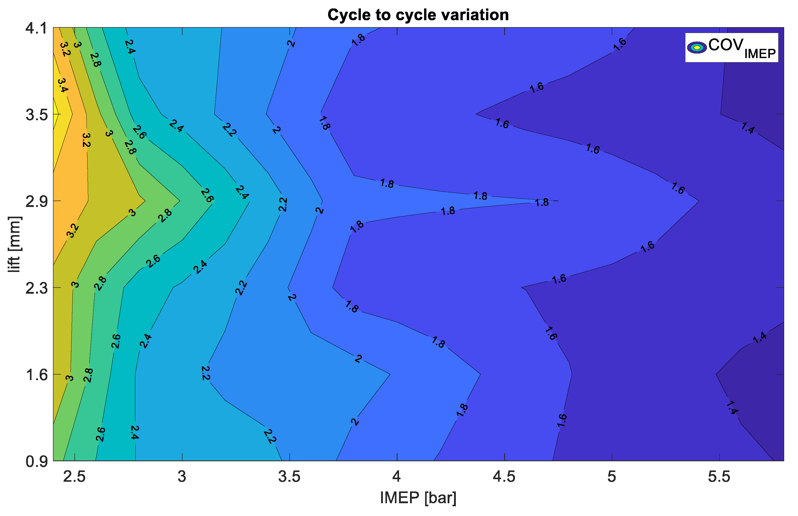
Cycle-to-cycle-variation is shown in Figure 6. It depicts the coefficient of variation (COV) of IMEP as a function of lift and IMEP. The COVIMEP was calculated according to Equation (3) and was evaluated for 167 consequently recorded cycles.
C O V I M E P = s t d ( I M E P ) m e a n ( I M E P ) × 100
No significant influence on lift/IVC on cycle-to-cycle-variation was observed; COVIMEP depends mainly on the in cylinder mass. All levels were unproblematic as it is usually accepted that COVIMEP values below 5% lead to very smooth engine operation. It must be mentioned that cyclic variation can be more prominently influenced by changing the valve overlap, which was not done in this analysis.

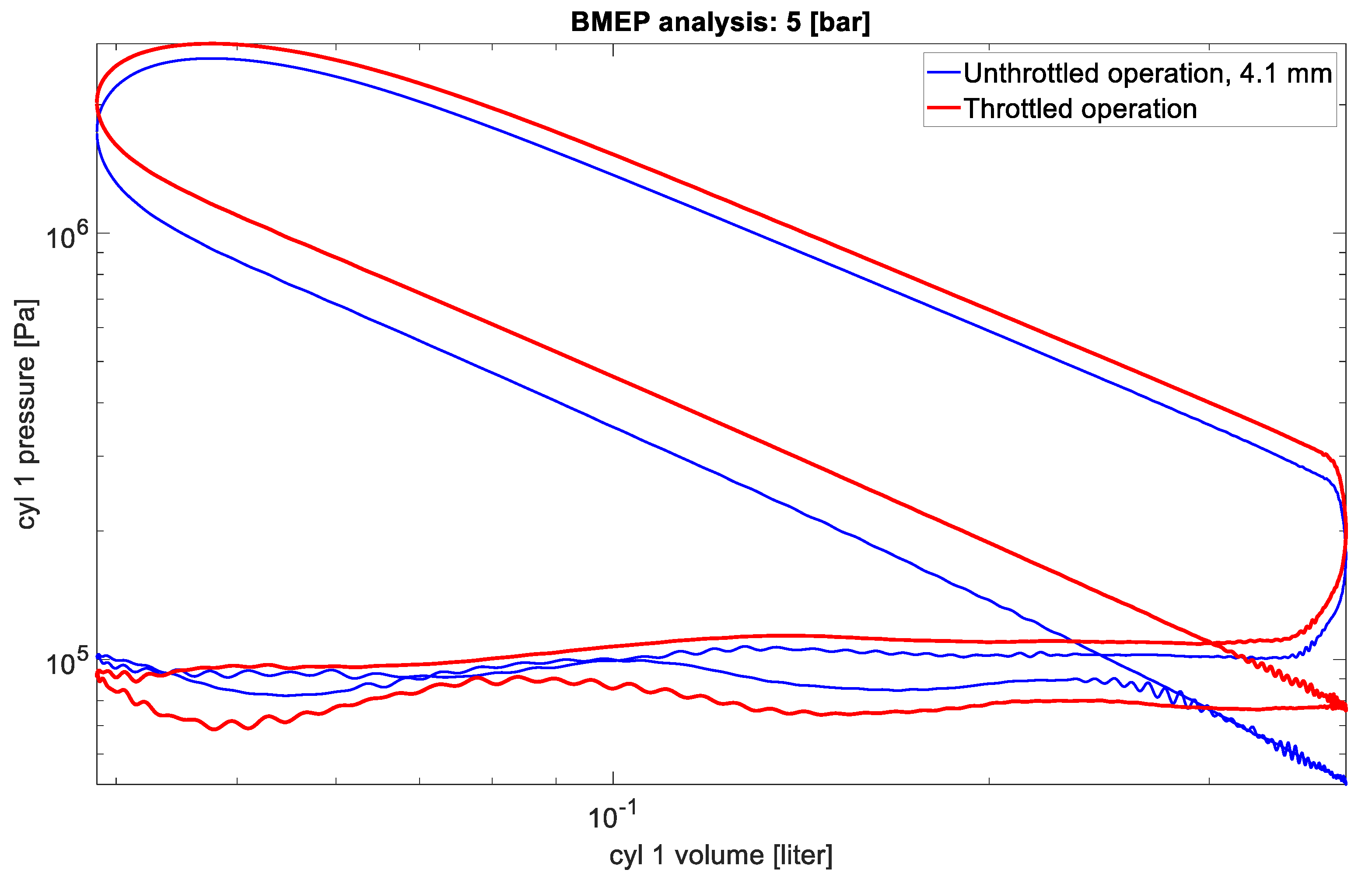
4.2. Throttled versus Unthrottled Operation

Measurements were made to compare the standard throttled Otto cycle, where IVC is set to 200 °CA and load is controlled by adjusting the pressure in the intake manifold, with the Miller cycle where the intake valve timing is adjusted while the throttle upstream the intake manifold remains open. Table 4 lists, for three IMEP values, the indicated efficiencies and the pumping losses for the throttled Otto cycles, as well as for the Miller cycles using best efficiency IVC lift/timing combinations.
For all three IMEP values (2.5, 3.5 and 4.5 bar) significant fuel savings were achieved using Miller cycles instead of throttled operation.
Figure 7 depicts the pressure volume diagram of the throttled and unthrottled case for 4 bar BMEP.
Even at medium load, where the differences in pumping losses are low (0.3 and 0.06 bar), an improvement in efficiency of 3.9% was recorded. This suggests that the combustion deterioration losses due to lack of turbulence are often overestimated or mitigated by other factors.

4.3. Willans Approximation to Decouple Thermal Efficiency and Pumping Losses

Typically, the energetic behavior of an energy conversion or transmission device is described by its efficiency, which is the ratio of the useful to the invested energy. Energy conversion devices always have intrinsic dissipative losses, which means that they need a certain input to cover dissipation, even if no output is delivered. This leads to nonlinear efficiency versus load curves, especially towards low output. In order to systematically analyze the energetic input-to-output behavior of an energy conversion device, the direct representation of output versus input-energy turns out to be much more meaningful than the study of the efficiency, or the specific fuel consumption, versus load. This kind of representation is usually called a “Willans plot” [21], referring to observations of Peter Willans [22], who saw in the late 19th century that input versus output power on high-speed steam engines can be represented by an affine relationship.
Equation (3) outlines the affine Willans approximation for internal combustion engines, which returns the IMEP (output) as a function of fuel mean effective pressure (FuelMEP, input). PMEP represents the gas exchange losses (calculated as stated in previous chapter) and the Willans efficiency (ew) represents the thermodynamic properties of the engine [17].
I M E P 1 V d p d V = e w F u e l M E P 2 · m ˙ f u e l · L H V n · V d P M E P n e g a t i v e   a r e a p v   d i a g r a m
FuelMEP, which is proportional to the fuel quantity, can be interpreted as the IMEP level an engine would deliver without pumping losses (PMEP = 0) and with a hypothetical efficiency of 100% (ew = 1, i.e., perfect conversion of the fuel’s thermal energy into work) [17]. The Willans efficiency ew can be interpreted as the engine’s “inner efficiency” driven by the quality of the thermodynamic cycle.
Equation (4) outlines the energy conservation equation for a control volume that surrounds the engine [19].
m ˙ f u e l Q L H V = P p + Q ˙ w + H ˙ e + H ˙ e , i c
The fuel energy power calculated with the fuel mass flow ( m ˙ f u e l ) and fuel lower heating value ( Q L H V ) is divided between power delivered to the pistons (Pp), wall heat losses ( Q ˙ w ), exhaust enthalpy ( H ˙ e ), and exhaust enthalpy loss due to incomplete combustion ( H ˙ e , i c ). By integrating Equation (4) over one engine cycle and dividing it by the displacement volume ( V d ), the specific per cycle mean effective pressures were derived. Equation (5) outlines the energy equation in mean effective pressure terms.
F u e l M E P = I M E P + Q w M E P + H e M E P + H e , i c M E P F u e l M E P = I M E P + + P M E P + Q w M E P + H e M E P + H e , i c M E P
In Equation (5), the IMEP is further divided into positive IMEP (IMEP+) and PMEP. The remaining terms are wall heat losses mean effective pressure (MEP), incomplete combustion enthalpy MEP, and exhaust enthalpy MEP. The latter was calculated according to Equation (6) [17]. The temperature used in Equation (6) is the one measured at exhaust manifold entrance and the mass (m) is the total mass flowing through the engine in one engine cycle.
H e M E P = c p m T V d c p = { 573   T 0.097 T < 700 K 392   T 0.155 T > 700 K
Since precise calculation of wall heat losses and incomplete combustion enthalpy need complex modeling, these two terms were combined and named rest heat losses mean effective pressure ( Q r e s t M E P ). They were calculated as the remaining part of the FuelMEP according to Equation (7).
Q r e s t M E P = F u e l M E P Q E M E P I M E P
This approximation is valid for two reasons. First, the remaining term is mostly dependent on the wall heat losses, which normally have a minimum share of 20% of fuel energy compared to a maximal share of incomplete combustion of 5% [19]. Second, both wall heat losses and incomplete combustion (quenching and blowby) are expected to decrease for lower pressures and temperatures. For the same load, shorter IVC time with higher lift results in lower pressures and therefore lower temperatures, reducing the wall heat losses. For lower pressure, the amount of fuel in the crevice volume and the amount of leakage decreased, lowering the incomplete combustion enthalpy.
As the Willans approximation was used to split the influences into pumping losses and fuel conversion efficiency at constant IMEP, it allowed us to separate the effect that early IVC has on gas exchange and thermodynamic properties. 
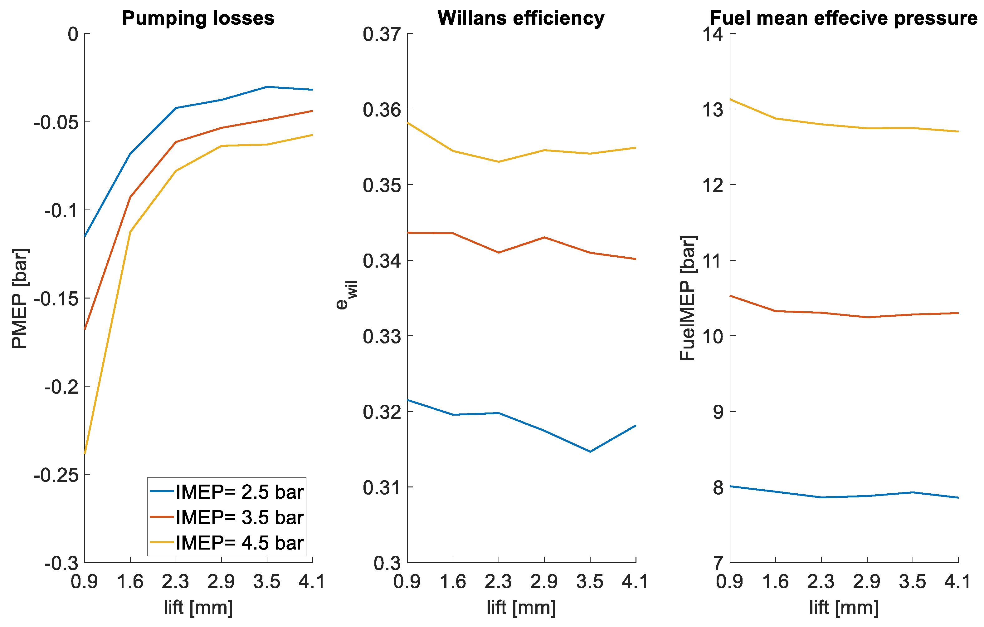
Figure 8 depicts, from left to right, the pumping losses PMEP, the Willans efficiency ew, and the fuel mean effective pressure FuelMEP as a function of lift for three different IMEP.
Higher Willans efficiency was reached at higher IMEP because higher in cylinder mass generally results in better Willans conversion efficiency. The Willans efficiency at constant IMEP slightly decreased with higher valve lifts (earlier IVC), which was a combined effect of slower combustion, lower heat losses (detailed discussion see below), and lower in cylinder mass. As expected, when using early IVC to control the load a clear reduction in PMEP was visible at higher lifts, and therefore earlier IVC for all three IMEP. FuelMEP decreased with increasing valve lift (earlier IVC) and, since FuelMEP is proportional to the fuel use, this suggest that increasing valve lift (earlier IVC) has a net beneficial effect.
The variations in Willans efficiency are driven by various influences. 
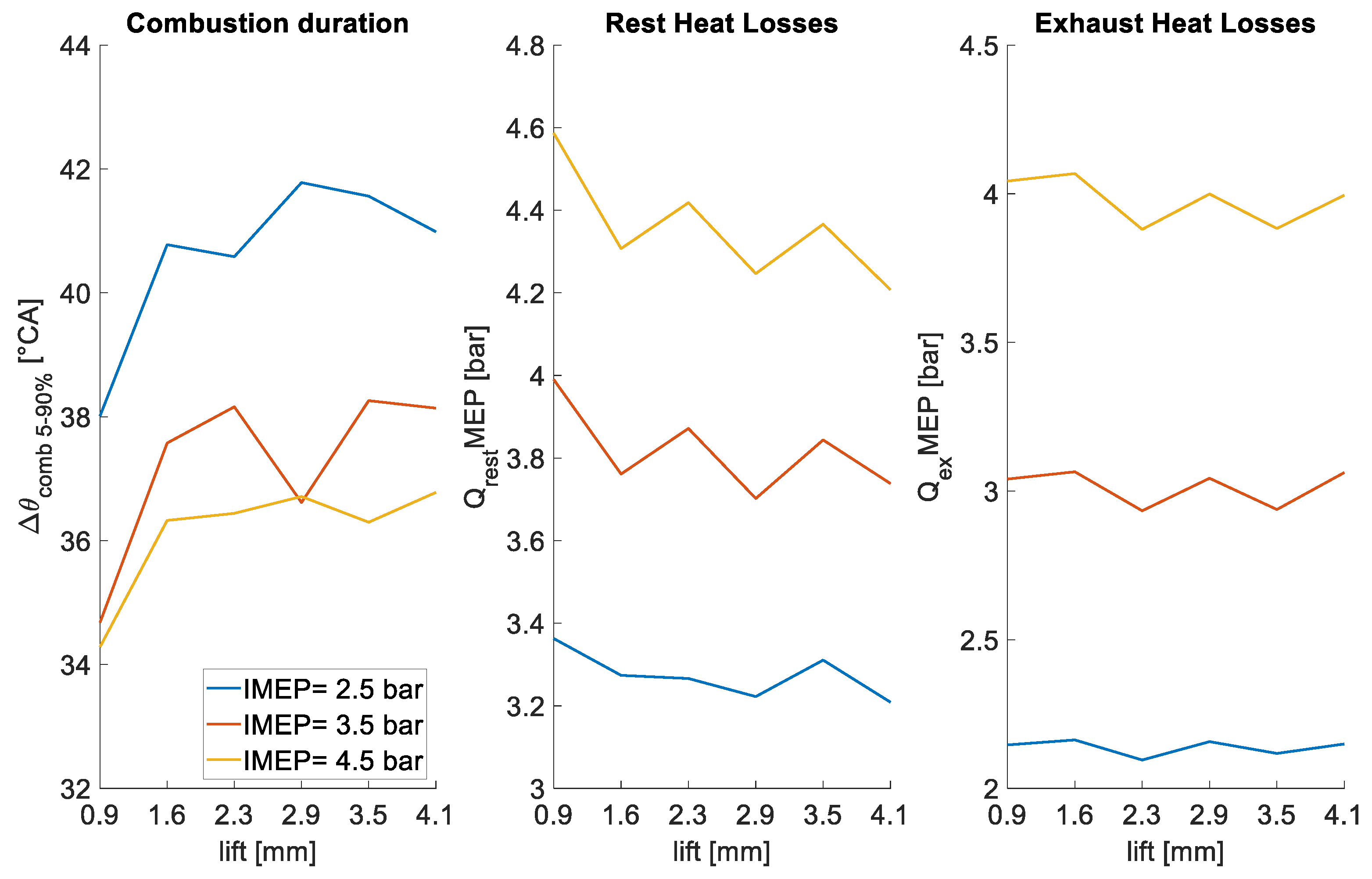
Figure 9 illustrates some factors affecting these variations. It depicts, from left to right, the combustion duration, the rest heat losses mean effective pressure (composed from wall heat losses and incomplete combustion), and the exhaust heat losses mean effective pressure as a function of intake valve lift for the three IMEP levels discussed.
An increase in combustion duration was observed at constant IMEP for higher lifts because of the aforementioned turbulence decrease with earlier IVC, which reduce the Willans efficiency. At the same time, the wall heat losses for higher lifts decreased and the exhaust heat losses remained approximately constant. The combined effect was, as shown in Figure 8, a slight reduction of the Willans efficiency.
Based on the Willans analysis for the engine considered, it can be concluded that the positive effect on engine efficiency of reducing pumping losses with early IVC is stronger than the losses attributed to early IVC. A tradeoff, or at least an attenuation of the disadvantage of the slightly less efficient combustion, can be recognized in the variation of the heat losses and in the incomplete combustion due to the lower pressures and temperatures achieved with early IVC. This experimental observation is in opposition to some results from the literature [7,23].

4.4. Engine Energy Balance

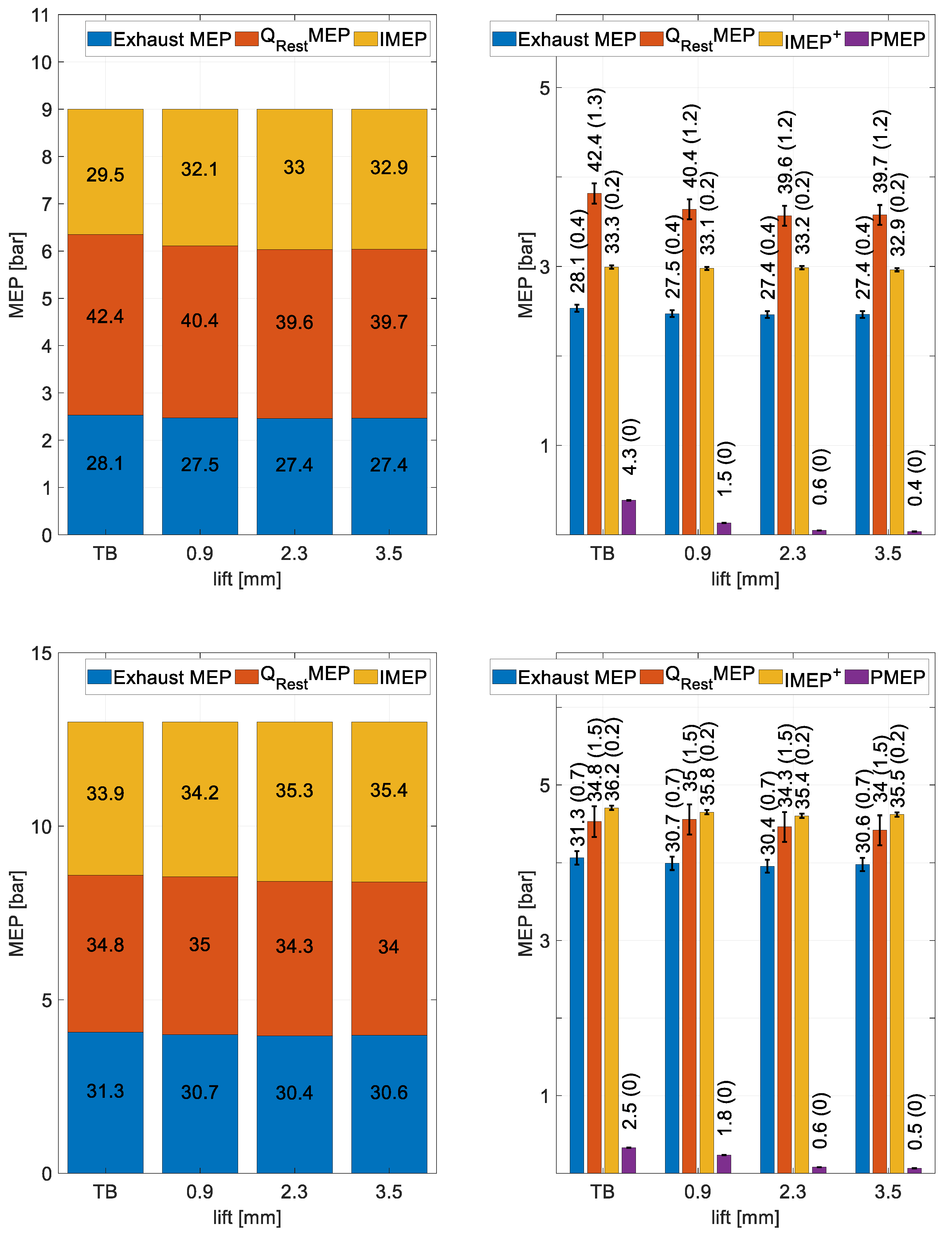
Variation in the Willans efficiency at constant IMEP and different IVC lift combination depend on the variation of in cylinder mass, combustion deterioration, exhaust heat losses, wall heat losses, and incomplete combustion heat losses. In order to interpret the influences driving the efficiency variation, an energy balance analysis was carried out for a constant FuelMEP level. Since FuelMEP is directly proportional to the fuel mass and the engine is strictly run at λ = 1, this resulted in a constant in cylinder air- and fuel mass. For this analysis, the losses arising from wall heat losses and incomplete combustion were grouped together into rest heat MEP. In this way, the FuelMEP (i.e., the hypothetical IMEP a 100% efficient engine would produce) was divided between IMEP, exhaust heat MEP, and rest heat MEP.
Figure 10 shows this analysis for 9 bar and 13 bar FuelMEP. On the left sides, the FuelMEP was divided into exhaust heat MEP, IMEP, and the rest heat MEP. On the right side, the IMEP was further split into positive IMEP and PMEP. Four points with the same FuelMEP were compared. The first point represents throttled operation (TB), the remaining ones represents three Miller cycles achieved with increasing valve lift (therefore earlier IVC). The right plot in Figure 10 shows, beside the division between the different terms of the energy balance, their relative experimental uncertainties as a percentage of FuelMEP, which was calculated according to Equation (1). IMEP and PMEP uncertainty arises only from pressure measurement, whereas the exhaust MEP uncertainty is derived from the air to fuel ratio, fuel mass flow, and exhaust temperature measurements. The remaining MEP uncertainty is derived from the sum of the previous uncertainties and from the FuelMEP uncertainty, which depends on air to fuel ratio, fuel mass flow, and lower heating value measurements.
On the left side in Figure 10, the increase in IMEP (from left to right columns) depicts the increase in indicated efficiency with higher valve lift (earlier IVC). To compensate for this effect, both wall heat losses MEP and exhaust heat MEP decreased. As the right side shows, the increase in efficiency was dominated by the reduction in PMEP. In spite of the fact that the wall heat losses and the exhaust heat losses decreased, the positive IMEP slightly decreased with higher valve lift (earlier IVC) because of the turbulence effect discussed.

5. Conclusions

This paper presents the experimental results achieved by applying early IVC (Miller cycle) to a four-cylinder engine operated with natural gas and fitted with a fully variable electro-hydraulic valve train. The focus of the work presented is the effect of IVC at low loads, and IVC effects on boosted operation were not considered. Loads ranging from 1.5 up to 5 bar BMEP were achieved in unthrottled operation with different combinations of IVC and intake lift, and the results were compared to throttled operation. Pumping losses reduction achieved with early IVC explains the efficiency gains achievable using early IVC. An indicated efficiency increase of up to 10% was observed when compared to throttled operations using high lift with an early IVC angle. Efficiency increases of up to 3% were observed by comparing unthrottled operations with higher lifts. As expected, a longer combustion duration resulted from earlier IVC angles. The earlier the valve closes, the more the lack of turbulence during combustion slows down the flame propagation. Therefore, the heat supply is less efficient. To understand the net effects, a Willans approximation was used to split the influences into pumping losses and fuel conversion efficiency at constant IMEP for various IVC and lift combinations. The Willans efficiency decrease for earlier IVC angles was weaker than expected, the reason being that multiple factors affect the Willans efficiency variation (in cylinder mass, heat losses, and combustion efficiency). The simplified energy balance for constant FuelMEP outlines that the earlier IVC angles lower heat losses (wall, incomplete combustion and exhaust ones), since early IVC strategies reduce in-cylinder temperature levels. For example, at low loads (ca. 3 bar IMEP), by advancing IVC the combustion deterioration was almost completely compensated by the reduction in heat losses so that the effect of reduced pumping losses with early IVC is fully exploited.
Studies in the literature typically report a tradeoff between pumping losses and combustion deterioration for premixed combustion [4,7,23]. The present experimental research shows that the behavior of the heat losses is an additional factor that also has to be considered, as it plays an important role in the overall energy balance. It can therefore be concluded that early IVC does not only reduce turbulence (therefore increasing combustion duration), but it also lowers pressure and temperature, thus leading to a significant reduction in wall heat losses, blowby, incomplete combustion, and also exhaust gas temperature.

Author Contributions

Conceptualization, M.B., N.Z. and P.S.; formal analysis, M.B, L.M.; writing—original draft preparation, M.B.; writing—review and editing, L.M. and P.S.; visualization, M.B.; supervision, N.Z. and P.S.; funding acquisition, P.S. All authors have read and agreed to the published version of the manuscript.

Funding

This research is part of the project “FlexWork” which is funded by the Swiss Federal Office of Energy, grant number SI/501619-01.

Acknowledgments

The authors express their gratitude to Wolfgang Schneider (Wolfgang Schneider Ingenieurbüro, Thun) and Andyn Omanovic (Empa) for their contributions in inventing and realizing the electro hydraulic valve train. Special thanks go also to the technical staff of Empa (H. Ehrensperger, R. Spühler, R. Graf) who set-up the experiments and modified the engine with great care.

Conflicts of Interest

The authors declare no conflict of interest.

Appendix A

The flow through a valve can be described through the isenthalpic orifice equation for compressible fluids. The approximation is valid for constant isentropic coefficient of 1.4 and a pressure ratio over the valve bigger then 0.5. Furthermore, the approximation assumes no losses in the accelerating part and fully turbulent flow after the narrowest point. The mass flow depends on the upstream ( p i n ) and downstream ( p o u t ) pressure of the valve, as well as on the area of the valve (A), the discharge coefficient ( c d ), and the fluid density ( ρ ) according to Equation (A1) [17].
m ˙ ( t ) c d A ( t ) 2 ρ   p o u t [ 1   p o u t   p i n ]

Appendix B

The burned rate variation was analyzed following the procedure outlined in [15]. With this methodology, the combustion characteristic was evaluated through the mass fraction burned (xB), which was estimated from the cylinder pressure trace (p), the volume (V), and from the per cylinder per cycle mass flow (m). By neglecting quenching, the fuel energy converted ( Q f ) is transferred to the gas ( Q n ) and partially to the walls ( Q w ). The heat transferred to the gas (Equation (A2)) was approximated using Rassweiler and Withrow’s assumption [10].
Q n = m c v ( T i + 1 T i ) = c v R V i + 1 [ p i + 1 p i ( V i V i + 1 ) k ]
The heat transferred to the wall was approximated with Hohenberg’s assumption (Equation (A3)) where n is the engine speed and α is the angular increment. The heat transfer coefficient ( α w ) was calculated as a function of in cylinder pressure (p), temperature (T), volume (V), and mean piston speed ( c m ).
Q w = [ α w A w ( T T w ) ] α 6 n α w = 0.0013 V 0.06 p 0.8 T 0.4 ( c m + 1.4 ) 0.8   J / m 2 K
The temperature (T) isentropic coefficient (k) and the specific heat at constant volume/pressure ( c v / c p ) were calculated according to Equation (A4).
T i = p i V i m R k = c p c v c v = 700 + 0.255 T   [ J / k g K ]
This methodology returns the mass fraction burned as a function of the crank angle, as shown in Equation (A5).
x B ( θ i ) = 0 i Q f 0 N Q f = 0 i Q n + Q w 0 N Q n + Q w
The heat release rate was calculated, from spark to bottom dead center, on the expansion stroke. The calculations were discreetly done in 0.2 °CA steps using measurements at the current angle (subscript i) and on the next discrete value (subscript i+1). The end of combustion wass set at the location of the first negative chemical fuel heat release transferred to the gas (subscript n) [24].
The two blue lines in Figure A1 represent the heat release rate (full line) and the wall heat losses (dashed line). The red points depict the mass fraction burned evolution calculated according to Equation (A5) for a 5 bar BMEP achieved with a 0.9 mm lift and an IVC angle of 155 °CA.
Figure A1. Mass fraction burned calculation.
Energies 13 01682 g0a1

References

  1. Zsiga, N.; Omanovic, A.; Soltic, P.; Schneider, W. Functionality and Potential of a New Electrohydraulic Valve Train. MTZ Worldw. 2019, 80, 18–27. [Google Scholar] [CrossRef]
  2. Zsiga, N.; Soltic, P.; Schneider, W. FlexWork—Lastregelung bei einem Motor mit elektrohydraulischem, vollvariablen Ventiltrieb. Presented at the Ladungswechsel und Emissionierung, 11, Stuttgart, Germany, 24 October 2018. [Google Scholar]
  3. Shiao, Y.; Dat, L.V. Efficiency Improvement for an Unthrottled SI Engine at Part Load. Int. J. Automot. Technol. 2012, 13, 885–893. [Google Scholar] [CrossRef]
  4. Li, T.; Gao, Y.; Wang, J.; Chen, Z. The Miller cycle effects on improvement of fuel economy in a highly boosted, high compression ratio, direct-injection gasoline engine: EIVC vs. LIVC. Energy Convers. Manag. 2014, 79, 59–65. [Google Scholar] [CrossRef]
  5. Lanzanova, T.; Nora, M.D.; Zhao, H. Investigation of Early and Late Intake Valve Closure Strategies for Load Control in a Spark Ignition Ethanol Engine. SAE Int. J. Engines 2017, 10, 858–872. [Google Scholar] [CrossRef]
  6. Schmitt, M.; Hu, R.; Wright, Y.M.; Soltic, P.; Boulouchos, K. Multiple Cycle LES Simulations of a Direct Injection Natural Gas Engine. Flow Turbul. Combust. 2015, 95, 645–668. [Google Scholar] [CrossRef]
  7. Knop, V.; Mattioli, L. An analysis of limits for part load efficiency improvement with VVA devices. Energy Convers. Manag. 2015, 105, 1006–1016. [Google Scholar] [CrossRef]
  8. Unger, H.; Schwarz, C.; Schneider, J.; Koch, K.-F. The Valvetronic: Experience from Seven Years of Mass Production and a Discussion of Future Prospects. MTZ Worldw. 2008, 69, 30–37. [Google Scholar] [CrossRef]
  9. Luttermann, C.; Schünemann, E.; Klauer, N. Enhanced VALVETRONIC Technology for Meeting SULEV Emission Requirements. SAE Technol. Pap. 2010, 1, 7. [Google Scholar] [CrossRef]
  10. Mendera, M.S.K.Z.; Spyra, A. Mass fraction burned analysis. J. KONES Intern. Combust. Engines 2002, 3, 193–201. [Google Scholar]
  11. Soltic, P.; Hilfiker, T.; Hänggi, S. Efficient light-duty engine using turbulent jet ignition of lean methane mixtures. Int. J. Engine Res. 2019, 70, 123–134. [Google Scholar] [CrossRef]
  12. Schechter, M.M.; Levin, M.B. Camless Engine. SAE Tech. Pap. 1996. [Google Scholar] [CrossRef]
  13. Zsiga, N.; Omanovic, A.; Soltic, P.; Schneider, W. Wirkungsgradvorteile beim Ottomotor unter Verwendung einer nockenwellenlosen, vollvariablen Ventilsteuerung gegenüber gedrosseltem Betrieb. Presented at the 8, VDI-Tagung Ventiltrieb und Zylinderkopf, Würzburg, Germany, 25 June 2019. [Google Scholar]
  14. Chiang, C.J.; Yang, J.L.; Lan, S.Y.; Shei, T.W.; Chiang, W.S.; Chen, B.L. Dynamic modeling of a SI/HCCI free-piston engine generator with electric mechanical valves. Appl. Energy 2013, 102, 336–346. [Google Scholar] [CrossRef]
  15. Tomić, M.V. A quick, simplified approach to the evaluation of combustion rate from an internal combustion engine indicator diagram. Therm. Sci. 2008, 12, 85–102. [Google Scholar] [CrossRef]
  16. Shelby, M.H.; Stein, R.A.; Warren, C.C. A New Analysis Method for Accurate Accounting of IC Engine Pumping Work and Indicated Work. Presented at the SAE 2004 World Congress & Exhibition, Detroit, MI, USA, 8–11 March 2004. [Google Scholar] [CrossRef]
  17. Guzzella, L.; Onder, C.H. Introduction to Modeling and Control of Internal Combustion Engine Systems; Springer Science & Business Media: Berlin, Germany, 2010. [Google Scholar]
  18. Weberbauer, F.; Rauscher, M.; Kulzer, A.; Knopf, M.; Bargende, M. Generally Applicate Split of Losses for New Combustion Concepts. MTZ Worldw. 2005, 66, 17–19. [Google Scholar] [CrossRef]
  19. Heywood, J.B. Internal Combustion Engine Fundamentals; McGraw-Hill: New York, NY, USA, 1988. [Google Scholar]
  20. Zhao, J.; Xi, Q.; Wang, S.; Wang, S. Improving the partial-load fuel economy of 4-cylinder SI engines by combining variable valve timing and cylinder-deactivation through double intake manifolds. Appl. Therm. Eng. 2018, 141, 245–256. [Google Scholar] [CrossRef]
  21. Greene, A.B.; Lucas, G.G. The Testing on Internal Combustion Engines; English University Publisher: London, UK, 1969. [Google Scholar]
  22. Hills, R.L. Power from Steam: A History of the Stationary Steam Engine; Cambridge University Press: Cambridge, UK, 1989. [Google Scholar]
  23. Sun, T. Experimental research on pumping losses and combustion performance in an unthrottled spark ignition engine. Proc. Inst. Mech. Eng. Part A J. Power Energy 2018, 232, 888–897. [Google Scholar] [CrossRef]
  24. Central, P. Combustion analysis and cycle-by-cycle variations in spark ignition engine combustion Part I: An evaluation of combustion analysis routines by reference to model data. Proc. Inst. Mech. Eng. Part D J. Automob. Eng. 1998, 212, 381–399. [Google Scholar]
Figure 1. Electro hydraulic valve train on the VW EA111 short block (left), engine on the test bench (right).
Energies 13 01682 g001
Figure 2. Scheme of the engine’s and valve train’s setup.
Energies 13 01682 g002
Figure 3. Measured valve lift profiles for different lift- and duration setting of the intake valves.
Energies 13 01682 g003
Figure 4. Analysis of efficiency and pumping losses at an engine speed of 2000 min−1.
Energies 13 01682 g004
Figure 5. Combustion duration and IVC angle.
Energies 13 01682 g005
Figure 6. Cycle to cycle variation.
Energies 13 01682 g006
Figure 7. Pressure volume diagramm.
Energies 13 01682 g007
Figure 8. Willans pararameters.
Energies 13 01682 g008
Figure 9. Influence of intake valve lift on Willans efficiency.
Energies 13 01682 g009
Figure 10. Energy balance at 9 bar (above) and 13 bar (below) FuelMEP for throttled (TB) operation and three levels of valve lift (three values of IVC).
Energies 13 01682 g010
Table 1. Main characteristics of the experimental setup.
Engine basisVolkswagen 1.4 L, production code EA111
Bore/stroke/number of cylinders76.5 mm/75.6 mm/4
Compression ratio10
FuelingPort fuel injection of natural gas using Bosch NGI2 injectors
Valve trainSelf-developed, electrohydraulic, water-glycol (engine coolant) used as the hydraulic working fluid
Engine controlRapid prototyping system (dSPACE)
In-cylinder pressure transducersM10 Piezoelectric, water-cooled (Kistler 6061B)
Stoichiometry sensorWide band (Bosch LSU 4.9)
Valve lift measurementLinear encoders (Elgo Electronic), using custom-developed converters
Test benchHoriba Dynas LI250
Test bench automationHoriba STARS Engine
Torque measurementHBM T40 torque transducer
Fuel flow measurementCoriolis sensor (Rheonik RHM015)
Combustion air flow measurementABB Sensyflow P
Emission measurement systemHoriba Mexa-One-D1-EGR
Table 2. Measurements uncertainty.
MeasurementUncertainty
Fuel mass flow { 0.2 %   m a s s   f l o w > 1.8 k g / h 0.5 %   m a s s   f l o w < 1.8 k g / h
Cylinder pressure0.6%
Air to fuel ratio0.7%
Lower Heating Value0.1%
Exhaust Gas Temperature0.4%
Table 3. pV diagram experiments details. IVC – intake valve closing; PMEP – pumping mean effective pressure.
BlueRedGreen
IVC111 °CA97 °CA84 °CA
Lift0.9 mm1.6 mm4.1 mm
PMEP0.190 bar0.099 bar0.047 bar
η i n d 33.6%34.6%34.4%
Table 4. Comparison between throttled and unthrottled operation.
IMEP [bar]Indicated EfficiencyPumping Losses [bar]Fuel Saving Compared to Throttled Operation
Throttled Otto cycles2.528.8%0.389
3.532.1%0.365
4.534.0%0.324
Unthrottled Miller cycles2.531.8%0.0329.4%
3.534.1%0.0536.1%
4.535.4%0.0573.9%

