Understanding the Role of Optimized Land Use/Land Cover Components in Mitigating Summertime Intra-Surface Urban Heat Island Effect: A Study on Downtown Shanghai, China

Abstract

In this study, 167 land parcels of downtown Shanghai, China, were used to investigate the relationship between parcel-level land use/land cover (LULC) components and associated summertime intra-surface urban heat island (SUHI) effect, and further analyze the potential of mitigating summertime intra-SUHI effect through the optimized LULC components, by integrating a thermal sharpening method combining the Landsat-8 thermal band 10 data and high-resolution Quickbird image, statistical analysis, and nonlinear programming with constraints. The results show the remarkable variations in intra-surface urban heat island (SUHI) effect, which was measured with the mean parcel-level blackbody sensible heat flux in kW per ha (Mean_pc_BBF). Through measuring the relative importance of each specific predictor in terms of their contributions to changing Mean_pc_BBF, the influence of parcel-level LULC components on excess surface flux of heat energy to the atmosphere was estimated using the partial least square regression (PLSR) model. Analysis of the present and optimized parcel-level LULC components and their contribution to the associated Mean_pc_BBF were comparable between land parcels with varying sizes. Furthermore, focusing on the gap between the present and ideally optimized area proportions of parcel-level LULC components towards minimizing the Mean_pc_BBF, the uncertainties arising from the datasets and methods, as well as the implications for sustainable land development and mitigating the UHI effect were discussed.

1. Introduction

It is projected that global urban dwellers will increase from the present 55% to 68% in 2050 [1]. The ongoing urbanization presents numerous challenges for the urban environment and human well-being [2,3], as evidenced by the dramatic land use/land cover (LULC) change for intensive human settlements inevitably altered hydrological circulation, climate regulation, soil conservation, and biodiversity preservation [4,5,6,7,8,9,10,11]. One of the environmental consequences of LULC change is the urban heat island (UHI) effect. Associated with human activities and climate change [12,13,14,15,16,17,18,19], the UHI effect significantly affects emissions of air pollutants and greenhouse gases [20], meteorological disasters, and health risks [21,22].

Since the 1830s, the meteorological station recorded air temperature (AT) has been widely used to monitor the UHI effect at canopy height, due to the advantage of long time series data for historical climate analysis. Usually, the weather stations were sparsely and unevenly distributed within and around the cities. They are not fully representative to reveal the UHI effect of differing local climate zones [23], especially in the circumstance that urban encroachment in the suburban/rural area caused the biased AT recorded at local weather stations, which was known as the so-called “city-entering” phenomenon of stations [24]. The land surface temperature (LST) is used as an alternative to identify the surface urban heat island (SUHI) effect [25]. In contrast to local weather stations with low spatial coverage, the satellite-borne thermal sensors with a wide instantaneous field of view (IFOV) can capture the thermal features of land surface quickly and provide a cost-effective solution. Since the 1970s, the satellite-borne thermal remote sensing has been a promising approach for monitoring city-level and regional SUHI effect worldwide. So far, there has been well-documented literature on the application of satellite-borne thermal sensors for multiple-scale SUHI studies, using thermal infrared bands acquired from the low-resolution sensors (~km) such as Geostationary Operational Environmental Satellite (GOES), Advanced Very High-Resolution Radiometer (AVHRR) and Moderate-resolution Imaging Spectroradiometer (MODIS) and mediate resolution sensors (60–120 m) such as Landsat-5/Theme Mapper (TM), Landsat-7/Enhanced Theme Mapper Plus (ETM+), and Landsat-8/Thermal Infrared Sensor (TIRS), as well as Advanced Spaceborne Thermal Emission and Reflection Radiometer (ASTER) [26,27,28].

However, on the applicability of satellite thermal remote sensing for SUHI studies, two questions should be addressed (1) how to transfer the spatially explicit information of intra-SUHI effect to the decision-making of land development and land parcel design? and (2) how to link the LST-indicated SUHI effect with the well-known canopy UHI effect? On the first question, when we turned our researching of interest into the urban area, it was found that these low and mediate resolution thermal bands were not suitable for monitoring the SUHI effect in urban settings with diverse LULC components, various urban morphology, and fine-scale land parcel design attributes [29,30,31]. In practice, the Advanced Thermal and Land Applications Sensor (ATLAS) operated by the American National Aeronautics and Space Administration (NASA) can capture the fine-scale thermal property of urban LULC components. Unfortunately, such aerial high-resolution thermal images (~10 m) are costly and very lacking for most of the SUHI studies. On the other hand, several trial studies were performed to thermally sharpen the coarse MODIS or GOES data to simulate the thermal signals of Landsat TM/ETM+ and ASTER in the urban area, but the LST products were still too coarse to indicate the SUHI effect. Alternatively, the combined usage of the high-resolution satellite/aerial images and mediate resolution satellite TIR bands may provide a practical way of mapping the urban thermal environment [31]. On the second question, the direct linkage between the LST-indicated intra-SUHI effect with the canopy UHI effect may be subject to many uncertainties. As an alternative, the LST can be used to estimate the excess surface flux of heat energy to the atmosphere, which was closely related with the surface warming [32], and thus, can help illustrate the relationship between SUHI effect and canopy UHI effect.

Nowadays, urban areas, which are subject to local warming effect or the combined local and global warming effects, are the fundamental units for climate change adaptation and mitigation [33]. Thus, focusing on the relationship between LULC components and artificial modification of urban climate, how cities cope with the UHI effect optimizing land use patterns towards sustaining regional ecosystems, will significantly affect UHI mitigation and adaption to climate change [34,35,36,37,38,39,40].

Taking downtown Shanghai, for example, which suffers from summertime extreme heat events, as a case study, this study aims to investigate the relationship between parcel-level LULC components and summertime intra-SUHI effect, and further find the solution to cooling the city and mitigating summertime intra-SUHI effect through the optimized LULC components. We expect the findings of this study will be beneficial for decision-makers who are engaged in mitigating the UHI effect and adapting to climate change.

2. Location of the Study Area

Downtown Shanghai, the economic center of China, is located between latitudes 31°32′ N–31°27′ N and longitudes 120°52′ E–121°45′ E. This region has a northern subtropical monsoon climate. The average annual temperature approximates 15 °C, with temperatures averaging 28 °C in the summer and 4 °C in the winter. The average annual precipitation ranges between 1000 and 1200 mm, with approximately 60% of the rainfall being received during spring and autumn. It covers an area of 4000 km², housing approximately 84.03% of a total of 24.18 million permanent residents within the boundary of greater Shanghai [41]. In this study, concerning previous studies of urban function zones (UFZs) in China [42,43,44,45], four typical UFZs of downtown Shanghai were selected (see Figure 1 and

Table 1. Description of four UFZs.

UFZ	Area (km2)	Description
Wujiaochang	7.09	One of the subcenters of downtown Shanghai with a cluster featuring a commercial center, colleges and universities, and a high-tech park for innovative firms.
PeacePark	2.00	Featured with a cluster of high education, innovative enterprises, Peace park, and recreational landscaping.
UrbanCore	5.97	The heart of downtown Shanghai, with a cluster of municipal administrative services, banking, headquarter economy, commercial center, and historical and cultural resorts.
Xujiahui	2.58	One of the sub-centers of downtown Shanghai, featuring a cluster of a commercial center, historical and cultural resorts, high education, advanced medical care, and innovative enterprises.

).

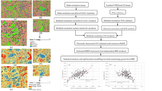
3. Materials and Methods

3.1. Materials

The data sources include the Landsat-8 images, high-resolution Quickbird image, and the auxiliary datasets. Due to the influence of cloud contamination, the available satellite images were limited. In this study, two cloud-free Landsat-8 satellite images (path/row:118/38) acquired on two summertime dates (August 13, 2013, and August 3, 2015), were used for retrieval of LST. A high-resolution Quickbird image (dated April 1, 2014) covering the four UFZs was used for the classification of LULC components. Together with the free-accessible Google Earth and Baidu Map, the commercial digitalized urban thematic maps of downtown Shanghai [46] were used as the auxiliary datasets.

3.2. Methods

To better illustrate our research aims and related arrangement of the sections, an overall technical flowchart containing the basic and key procedures employed for this study were shown in Figure 2.

3.2.1. Classification of LULC Components and Delimitation of Land Parcels

By using a land surface classification system with nine LULC types in downtown Shanghai [31], the classification of LULC components was performed with an object-oriented classification (OOC) method. This OOC method could make full use of contextual data—such as spectral information, texture, spatial neighborhood properties, and fractal dimensions—from very high-resolution images and delineate the objects of interest [47] with much higher accuracy than traditional per-pixel classification methods [48,49,50]. The overall accuracy is approximately 80.03%. The post-classification product was further manually corrected by overlapping it with Google Earth and Baidu Map layers and then validated in a field survey, with an overall correction accuracy of 91.1%. Subsequently, based on our prior knowledge of land use and the developmental intensity of the UFZs, 167 regular polygons were drawn to delimit the land parcels along the directional and geometric features of traffic roads, bounding walls, and urban creeks enclosing the clustered land units.

Herein, we want to emphasize that the classification of LULC components was used for the estimation of land surface emissivity. Given the mixing-pixel effect of the land surface showing the same/similar LST, and many LULC types may complicate the analysis between LULC components and the associated thermal effect, for this study, the nine LULC classes were aggregated into four classes: building (architecture with vertical walls and roofs, e.g., house and warehouse), paved surface (e.g., asphalt road, square, playground), waterbody (e.g., creek and pond), and vegetation (e.g., tree, shrub, and lawn) (see Figure 3).

3.2.2. Retrieval and Validation of High-Resolution Thermally Sharpened LST

In this study, retrieval and validation of high-resolution thermally sharpened LST include the following steps. Firstly, for Landsat 8 TIR bands, given band 11 is subject to higher uncertainty of telescope stray light disturbance [51,52], band 10 was used to generate the top of the atmosphere (TOA) radiance as follows,

$$L_{sensor,\lambda }=gain\times DN+offset,$$

(1)

where L_sensor,λ is the at-sensor radiance of thermal band pixels in W/(m² ster μm), the gain is the slope of the radiance/DN conversion function, and offset the slope of the radiance/DN conversion, respectively [53].

Secondly, a spatial interpolation-based method known as co-Kriging interpolation was employed to generate the high-resolution thermally sharpened LST, via a combination of the high-resolution land surface products and Landsat-8 TIR band 10 data [31]. Given the bias arising from the different resolutions between the high-resolution LULC components product and coarse TOA radiance data, both datasets must be scaled to the same resolution. Therefore, the high-resolution LULC components product were resampled with multiple resolutions (1–9 m) and set as the base maps to overlap and delimit the TOA radiance layer. We assumed that same/similar surfaces would have the same/similar radiance values since there is no available reference data for this study. Then, for each scene of the TOA radiance layer, we tried many times from hundreds of points per km² to 6000 points per km² to compare the co-Kriging interpolation results, and we found the remarkable decrease in the pairwise bias between the raw and simulated points in response to the increasing point number. It was found that the threshold of 3000 points was reasonable as the pairwise bias was inclined to get flat and changed little when the point number was greater than 3000 points [31]. Therefore, 3000 spatially random points per km² with the same interval as the multiple resolutions of the LULC component products were generated to extract the point-based radiance values falling within the polygon of each same/similar LULC category. The extracted points with radiance values were used to rebuild the TOA radiance layer, using the co-Kriging interpolation method. Besides, based on the multiple-resolution LULC layers, a surface emissivity correction for the same/similar LULC components was performed according to empirical studies [54,55] and laboratory testing [56]. Subsequently, based on a generalized single-channel method known as the range transfer equation (RTE) for retrieving LST [57], the emissivity corrected LST using was computed as follows,

$$L_{sensor,\mathsf{\lambda }}=\left[{\mathsf{\epsilon }}_{\mathsf{\lambda }}{B}_{\mathsf{\lambda }}\right(T_s)+(1-{\mathsf{\epsilon }}_{\mathsf{\lambda }})L_{atm,\lambda }^{\downarrow }]\times {\mathrm{Ʈ}}_{\mathsf{\lambda }}+L_{atm,\lambda }^{\uparrow }$$

(2)

$$B_{\mathsf{\lambda }}\left(T_S\right)=\frac{L_{sensor,\lambda }-L_{atm,\lambda }^{\uparrow }-{\mathrm{Ʈ}}_{\lambda }\times \left(1-{\epsilon }_{\lambda }\right)L_{atm,\lambda }^{\downarrow }}{{\mathrm{Ʈ}}_{\lambda }{\epsilon }_{\lambda }}$$

(3)

$$Ts=\frac{k_2}{\ln \left(1+\frac{k_1}{B_{\mathsf{\lambda }}\left(T_S\right)}\right)}$$

(4)

where B_λ(T_S) is the black body radiance given by Plank’s law, T_S the black body LST in Kelvin (K), ε_λ the corrected emissivity of the specific land surface (details see reference [31]).$L_{atm,\lambda }^{\downarrow }$ is the downwelling atmospheric radiance, $L_{atm,\lambda }^{\uparrow }$ the upwelling atmospheric radiance, Ʈ_λ the total atmospheric transmissivity between the surface and sensor, all of which were retrieved from a web-based Atmospheric Correction Tool [58]. k₂ and k₁ are band 10 thermal conversion constants included in the metadata file of Landsat 8 data [53].

Finally, validation for the sharpened LST products was performed by comparing the pixel-based root-mean-square error (RMSE) between the original 30 m LST products and the resampled 30 m products from the sharpened products (Appendix

Table A1. Pixel-based root-mean-square error (RMSE) between the original 30 m and the resampled 30 m LST products from the sharpened products (1–9 m).

	1m	3m	5m	7m	9m
Mean ± s.d.	2.51 ± 0.32a	2.71 ± 0.33a	2.83 ± 0.42a,b	2.90 ± 0.56a,b	3.20 ± 0.65 b

Note: The different labels denote significant difference at 0.05 level.

). The sharpened LST products at 1 m resolution were employed for further analysis due to their superior visual quality and minimal RMSE.

3.2.3. Estimation of Parcel-Level Sensible Heat Flux

Based on the high-resolution sharpened LST products, the parcel-level blackbody sensible heat flux (BBF) was estimated follows [32]:

$${\Phi }_{BBFD}={{\displaystyle \int }}_{10.60\mu m}^{11.19\mu m}\frac{C_1}{\pi {\lambda }^5\left[\exp \left(\frac{C_2}{\lambda T}\right)\right]}d\lambda$$

(5)

BBF_i = Φ_BBFD×A_i

(6)

where Φ_BBFD is the pixel-based BBFD (W·m⁻²), C₁ = 3.7404×10⁸ (W·μ⁴·m⁻²), C₂ = 14387, $\lambda$ is TOA radiance, and T is LST in Kelvin (K), A_i is area of the ith land parcel (m²).

However, due to the uneven size of the land parcels, there exists a remarkable variation of parcel-level BBF. Therefore, regardless of the size effect of land parcels, the parcel-level BBFs were converted to per ha BBF (pc_BBF), namely a cumulative number of the BBFD multiplying by the pixels within an idea parcel sized 1 ha, to make them comparable.

3.2.4. Statistical Analysis and Estimating the Optimized Lulc Components for Minimizing Mean_pc_BBF

As a regular step, the exploring data analysis procedure, including descriptive statistics, normality test, Box–Cox transformation for skewed data (if there were), and Pearson’s product-moment correlation, was performed. In this study, Pearson’s product-moment correlation analysis helped quantify the assumed relationship between the dependent and independent variables. However, the result of correlation analysis indicated the multicollinearity between the independent variables (for details see Section 4.1). Thus, the partial least square regression (PLSR) model that was developed for fixing the problem of the multilinearity was employed. Further, to avoid the over-fitting problem and determine a reasonable model with the appropriate number of components that has good predictive ability, the leave-one-out (LOO) method was used for cross-validation, by selecting the model with the highest average predicted R² and the lowest average prediction sum of squares (PRESS). The validated PLSR model was written as follows,

Mean_pc_BBF = α₁+β₁·X₁+β₂·X₂+β₃·X₃+β₂₃·X₂·X₃+β₄·X₄+ε,

(7)

where Mean_pc_BBF is the averaged pc_BBF of two summertime days since the overall parcel-level BBFD products on two dates were highly similar to each other (for details, see Appendix Figure A1), so were the pc_BBF; α₁ is the intercept/constant item, β₁~β₄ are the partial coefficients; X₁~X₄ are the Box–Cox transformed area proportions of the paved surface, waterbody, vegetation, and building within each land parcel, respectively (for details see Appendix

Table A2. Estimations of the lambda (λ) and formulas.

Box-Cox Transformed	Estimated Lambda (λ)	Formulas
X1	0.50	X1 = sqrt (Paved surface)
X2	0.11	$\mathrm{X}2=\frac{{\left(\mathrm{Water}\mathrm{body}\right)}^{0.11}}{0.89}$
X3	0.00	X3 = log (Vegetation)
X4	1.34	$\mathrm{X}2=\frac{{\left(\mathrm{Building}\right)}^{0.11}}{0.89}$

). ε is the error term.

Subsequently, based on the validated PLSR model, nonlinear programming with constraints towards minimizing Mean_pc_BBF through the optimized LULC components was written as follows,

Min α₁+β₁·X₁+β₂·X₂+β₃·X₃+β₂₃·X₂·X₃+β₄·X₄

(8)

$$\mathrm{s}.\mathrm{t}.X\prime 1+X\prime 2+X\prime 3+X\prime 4\le 100$$

(9)

$$s.t.\{\begin{array}{cc}X\prime 1+X\prime 2+X\prime 3+X\prime 4\le 100& \hfill \left(9\right)\\ \alpha 0+\beta \prime 1·X3+\beta \prime 2·X3^2+\beta \prime 3·X3^3\ge \mathrm{BBF}\_\mathrm{Threshold}& \hfill \left(10\right)\end{array}$$

(10)

where the definitions of α₁, β₁~β₄, X₁~X₄ are the same as Equation (7). X^’₁~X^’ ₄ are the raw area proportions of the paved surface, waterbody, vegetation, and building within each land parcel. α₀ is the constant item of the cubic regression model, β’₁~β’₃ are the coefficients. BBF_Threshold is the threshold value of pc_BBF in response to the changing area proportion of vegetation.

The statistical processes employed in this study were performed with R 3.6.2 [59] and the pls library for PLSR [60]. The Rsolnp library [61] was used to estimate the optimized LULC components for minimizing Mean_pc_BBF.

4. Results

4.1. Synoptic Analysis of Parcel-level LULC Components and Mean_pc_BBF

Overall, Figure 3 and Figure 4 show the highly similar patterns of parcel-level LULC components and associated intra-SUHI effect measured with Mean_pc_BBF at four UFZs. As shown in Figure 3, there were significant variations of parcel-level LULC components measured by their area proportions. The buildings occupied the highest area proportion of the land parcels (averaged 47.72%), followed by the paved surfaces (averaged 24.59%) and vegetation (averaged 23.98%), whereas waterbody occupied the lowest area proportion (averaged 1.25%). In response to the fragmented vegetation and waterbodies within the total landscape, Figure 4 shows the overall unevenly distributed pattern of Mean_pc_BBF. As shown, the clusters of pixels with a paved surface and dense buildings exhibited higher BBFD than the spatially sparse pixels with waterbodies and vegetation. By contrast, the aggregated pixels with dominant vegetation and waterbodies, such as the university campus, big parks, boulevards, and a few well-vegetated residential communities, exhibited significantly lower Mean_pc_BBF (65.24–72.00 kW, averaged 68.47 kW); whereas most of the parcels dominated with paved surfaces and dense buildings exhibited the mediate Mean_pc_BBF (68.10–72.38 kW, averaged 70.31 kW) to higher Mean_pc_BBF (68.50–74.56 kW, averaged 70.70 kW).

4.2. Interpretation of Relationship between Parcel-Level LULC Components and Mean_pc_BBF

In the sense of qualitative statistics,

Table 2. Coefficients of Pearson’s product-moment correlations.

Pairwise	Correlation
X2 (Waterbody) vs. X1 (Paved surface)	−0.166*
X3 (Vegetation) vs. X1 (Paved surface)	−0.312**
X4 (Building) vs. X1 (Paved surface)	−0.194*
X3 (Vegetation) vs. X2 (Waterbody)	0.503**
X4 (Building) vs. X2 (Waterbody)	−0.387**
X4 (Building) vs. X3 (Vegetation)	−0.611**
X1 (Paved surface) vs. Mean_pc_BBF	0.620**
X2 (Waterbody) vs. Mean_pc_BBF	−0.435**
X3 (Vegetation) vs. Mean_pc_BBF	−0.470**
X4 (Building) vs. Mean_pc_BBF	0.639**

Note: In this table, all the independent variables were Box–Cox transformed. * and ** denote significance at 0.05 and 0.01 levels, respectively.

shows the statistically significant relationships between the Box–Cox transformed parcel-level LULC components and the intra-SUHI effect measured with Mean_pc_BBF, as evidenced with the correlation coefficients indicating the multicollinearity that may mislead our understanding of the relationships as mentioned above. However, it can be seen that except for the positive relationship between X2 and X3, there were the negative relationships between the other LULC components, indicating the overall exclusive competition of land use purpose for urban land development and associated influence on Mean_pc_BBF. Figure 5 visually addresses the bivariate relationships between fine-scale parcel-level LULC components (e.g., building and vegetation) and Mean_pc_BBF. The observed positive/negative bivariate relationships with remarkable variations in Mean_pc_BBF are wholly in agreement with the heterogeneity of parcel-level LULC components and associated Mean_pc_BBF shown in Figure 3 and Figure 4. Based on Figure 5b, the BBF_Threshold in equation 10 was estimated.

Further, beyond addressing the bivariate relationships shown in Table 2 and Figure 5,

Table 3. Coefficients of partial least square regression (PLSR) models.

Variable	Coef	S-Coef
Constant	64.699	0
X1: Paved surface	0.417	0.267
X2: Waterbody	−0.464	−0.291
X3: Vegetation	0.562	0.085
X4: Building	0.019	0.741
Waterbody × Vegetation	−0.32	−0.196
Summary statistics	F = 51.340, p < 0.05
	Adjusted R2 = 0.561

Note: Coef and S-Coef denote unstandardized and standardized coefficients, respectively. In this table, all the independent variables were Box–Cox transformed.

comprehensively shows the quantitative relationship between the Box–Cox transformed parcel-level LULC components and their roles in controlling Mean_pc_BBF, explaining 56.1% variation of the Mean_pc_BBF associated with independent variables. As shown, along with the waterbody, the interaction of waterbody and vegetation exhibited the statistically significant negative coefficients, indicating their capacity for suppressing Mean_pc_BBF when fixing the other variables. In contrast, paved surface, vegetation, and building exhibited statistically significant positive coefficients, indicating their capacity for increasing Mean_pc_BBF. However, herein, the unstandardized coefficients (Coefs) of the Box–Cox transformed variables result in puzzling understanding as they cannot be directly comparable for indicating each specific positive/negative relationship with Mean_pc_BBF.

Alternatively, by measuring the changing standard deviation of Mean_pc_BBF in response to each one standard deviation increase in a given Box–Cox transformed variable, the standardized coefficients (S-Coefs) can better indicate the relative strength of the relationship between the Box–Cox transformed variables and Mean_pc_BBF. As indicated, the waterbody was found to be the strongest negative determinant of Mean_pc_BBF when fixing the other variables, as with each one standard deviation increase in waterbody would approximately decrease 0.291 standard deviations of Mean_pc_BBF. The interaction of waterbody and vegetation was found to be the second strongest negative determinant of Mean_pc_BBF when fixing the other variables, as with each one standard deviation increase in the interaction of waterbody and vegetation would approximately decrease 0.196 standard deviations of Mean_pc_BBF. Besides, vegetation was found to be the smallest positive determinant of Mean_pc_BBF when fixing the other variables, as with each one standard deviation increases in vegetation would approximately increase 0.085 standard deviations of Mean_pc_BBF. In contrast, when fixing the other variables, paved surface and building were found to be the mediate and highest positive determinants of Mean_pc_BBF, as with the relatively remarkable increase in standard deviations of Mean_pc_BBF, which respond to each one standard deviation increase in paved surface and building, respectively. The use of the S-Coefs made sense for the results.

4.3. Comparison of the Present and Optimized Parcel-level LULC Components and the Associated Mean_pc_BBF

Table 4. Changes in summertime Mean_pc_BBFs associated with present and optimized parcel-level LULC components.

	Area Proportion (%)		Mean_pc_BBF (kW)
LULC	Present	Optimized	Present	Optimized
Other	24.59	24.68	128.01	61.70
Waterbody	1.259	4.97
Vegetation	23.98	42.91
Building	47.72	27.44

shows the remarkable changes in summertime Mean_pc_BBFs associated with present and optimized parcel-level LULC components. As shown, except for the slight change of proportion of the other impervious surface in the present and optimized parcel-level LULC components, the changes in area proportions of the other LULC components were remarkable. As a whole, compared with present LULC components, the optimized parcel-level LULC components with the thresholding area proportions would cause an overall 51.80% decrease in summertime Mean_pc_BBFs.

On the other hand, if fixing the area portion of the other impervious surface constant, it is an excellent way to enhance the parcel-level area proportions of the waterbody and vegetation and simultaneously decrease area proportion of Building. However, due to the remarkable variation of parcel-level LULC components, there were only 7.79% of the land parcels (big parks and memorial cemetery), ultimately meeting the optimized thresholding area proportions of the parcel-level LULC components. In contrast, the land parcels with dominant impervious surface approximated 44.31% of total land parcels. Then, focusing on the gap between the present and ideally optimized area proportions of parcel-level LULC components, there would be higher uncertainties of minimizing the Mean_pc_BBF through adjusting urban land development and optimizing the parcel-level LULC components. How to seek practical solutions will be further emphasized in the discussion section.

5. Discussion

5.1. On the Data, Methods, and Findings of this Study

The occurrence of the intra-UHI effect depends on the complicated human-nature processes in the built environment. In addition to the macro-scale climate system, the micro-scale artificial modification of urban climate due to varying thermal properties of LULC is one of the key drivers of the intra-SUHI effect. Most of the datasets used in this study are publicly accessible, and statistical analysis methods and optimization algorithm adopted are well known among the researchers. Together with the spatial interpolation-based thermal sharpening method, which was proven to be capable to capture the varying thermal properties of fine-scale LULC components [31], the PLSR analysis quantitatively examined the relative importance of parcel-level LULC components in determining the Mean_pc_BBF. Furthermore, results of the present and optimized parcel-level LULC components and their contribution to the associated Mean_pc_BBF were comparable across the land parcels, regardless of their varying size.

In the existing studies for investigating SUHI effect via satellite thermal remote sensing, most of which only used the MODIS, Landsat TM/ETM+/8, and ASTER thermal band products [62,63], or additionally combined with high-resolution aerial photos/commercial satellite satellites for added interpretation [17,64,65], the results based on the unsharpened thermal band data were too coarse to examine the relationship between the observed LST and fine-scale LULC components. In contrast, our findings, though exhibiting the uncertainties of the Mean_pc_BBF between the present and ideally optimized area proportions of parcel-level LULC components, can provide more detailed information on the fine-scale intra-SUHI effect and optional choices for decision-making towards mitigating UHI effect. Thus, the application of the accessible public datasets and the methods in this study can be referenced to the case studies elsewhere.

5.2. Implications for Practical Solutions to Optimized Parcel-Level LULC Components towards Mitigating Intra-SUHI Effect

In the modern history of downtown Shanghai, this city was in the track of international trading and industrialization manipulated by the western colonialist authorities. This city’s compact form had been criticized for deteriorating the natural watery landscape and lacking green space during its growth [66]. In the period of ‘urban industrialization (1949–2000)’, this city became China’s biggest industrial center, and most of the land patches were encouraged for intensive development of industrial facilities, traffic roads, and residential quarters at the loss of the creeks and farmlands within the former urban-rural mosaics [67,68,69]. The resultant remnants of waterbodies and vegetation within urban areas accounted for tiny area proportions of downtown Shanghai, making this city a typically hot city during the summer.

Recently, with the growing awareness of the better environment, the local government has been dedicated to urban regeneration and improve this city’s green infrastructure via land replacement for new greenspace. The consequent increase in greenspace from 8278 ha in 1998 to 127,332 ha in 2015 was rewarded with a remarkable decrease in previous UHI hotspots [70,71,72]. However, as addressed in Section 4, the overall competitive parcel-level LULC components embodied the heterogeneity of urban land development intention and associated SUHI effect. As evidence, the cumulative area proportions of waterbodies and vegetation are still less than the recommended minimum 30% baseline of the study area, which can better interpret the weakness of present parcel-level waterbodies and vegetation in modifying the SUHI effect. To achieve the goal of minimizing Mean_pc_BBF, it is essential to trade-off the conflicts rooting in the facets of urban land development intention, then further reduce and remove the significant mismatching in area proportions between the present and optimized parcel-level LULC components. To do so, regeneration of the land parcels with dominant buildings and hard-top pavements well as architectural renovation should be officially given the top priority. For example, practice in ecological resilience, such as the well-managed vertical planting and roof garden, has exemplified its remarkable cooling capacity in microclimatic UHI mitigation. In addition to increasing the green ratio, it is crucial to shape the openness of urban morphology and alleviate the blocking of wind corridors that reduces convective heat removal and transfer by the wind [73]. We recommend that future land parcel design should guide the moderate density clusters of middle- and high-rises with acceptable building distance (e.g., 30 m or more, rather than merely the sunshine spacing).

5.3. Limitation of this Study and Future Researching Tasks

There are several noticeable shortcomings of this study. Firstly, due to the 16-day revisiting interval of Landsat 8 satellite and cloud contamination, only two cloud-free images are available for this study. Thus, the estimated parcel-level BBF, which was generated from the thermally sharpened LST products, can only capture the instantaneous field of view rather than the continuous scenes of the study area. Secondly, until the present, except for a few five-year intervals of aerial photography performed in earlier years, there have no available airborne sensors like the ATLAS at 10-m for investigating the BBF in downtown Shanghai. Alongside with lacking the airborne sensed data, the absence of in-situ measured parcel-level BBF datasets made the cross-validation of the estimated parcel-level BBF impossible. Thirdly, the three-dimensional features of urban morphology and their influences on micro-climate and human thermal comfort were not considered in this study. Consequently, in the sense of data demand for near real-time, temporal continuity, spatial representativeness, the direct linkage between the retrieved parcel-level BBF, human thermal comfort, and energy requirement for cooling was insufficiently illustrated. To fill these emphasized knowledge gaps, in future research design, the in-situ measurement of micro-climatic parameters, high-resolution land cover types, the three-dimensional features of urban morphology, should be incorporated into the computational fluid dynamics (CFD) simulation platforms (e.g., ENVI-met and WindperfectDX) to cross-validate the satellite observation and in-situ measurements, and then be further refined to generate the tempo-spatially continuous datasets.

In short, we argue that focusing on these above-mentioned shortcomings, to find the good questions and attempt to comprehensively put the conceived ideas into practice, then we can get close to the truth and find the practical ways to mitigate the adverse UHI effect and further enhance the adaption capacity to climate change.

6. Conclusions

Selecting downtown Shanghai as a case, this study quantitatively examined the influences of parcel-level LULC components on summertime intra-SUHI effect and further analyzed the potential of mitigating summertime intra-SUHI effect through the optimized LULC components. The major findings were summarized as follows,

(1) Overall, there exists a statistically significant relationship between fine-scale parcel-level LULC components and the intra-SUHI effect measured with Mean_pc_BBF. The observed remarkable variations in Mean_pc_BBF can be attributed to the heterogeneity of parcel-level LULC components.

(2) Focusing on the influence of parcel-level LULC components on intra-SUHI effect, the relative importance of waterbodies and vegetation in terms of their contributions to decreasing associated Mean_pc_BBF urgently require increasing their area proportions. Theoretically, the optimized parcel-level LULC components would cause an estimated 51.798% decrease in summertime Mean_pc_BBFs. However, how to balance the conflicts between the present and ideally optimized parcel-level LULC components towards minimizing the Mean_pc_BBF should be carefully considered. It is still a long and formidable challenge for decision-making of sustainable land development and mitigating the UHI effect.

(3) In contrast to the relative coarse scales of region and city levels, our study demonstrated a practical approach linking fine-scale parcel-level LULC components and intra-SUHI effect, using the integration of satellite-based thermal sharpening, statistical analysis, and nonlinear programming with constraints. The methodology and findings presented beneficial insights for guiding sustainable urban land development towards enhancing the city’s adaption capacity to climatic change for megacities like Shanghai.

References

1. United Nations. 2018 Revision of World Urbanization Prospects. Available online: https://www.un.org/development/desa/publications/2018-revision-of-world-urbanization-prospects.html (accessed on 20 November 2019).
2. Luck, M.; Wu, J. A gradient analysis of urban landscape pattern: A case study from the Phoenix metropolitan region, Arizona, USA. Landsc. Ecol. 2002, 17, 327–339. [Google Scholar] [CrossRef]
3. Li, J.; Song, C.; Cao, L.; Zhu, F.; Meng, X.; Wu, J. Impacts of landscape structure on surface urban heat islands: A case study of Shanghai, China. Remote Sens. Environ. 2011, 115, 3249–3263. [Google Scholar] [CrossRef]
4. Cai, Y.-B.; Li, H.-M.; Ye, X.-Y.; Zhang, H. Analyzing Three-Decadal Patterns of Land Use/Land Cover Change and Regional Ecosystem Services at the Landscape Level: Case Study of Two Coastal Metropolitan Regions, Eastern China. Sustainability 2016, 8, 773. [Google Scholar] [CrossRef] [Green Version]
5. Clerici, N.; Cote-Navarro, F.; Escobedo, F.J.; Rubiano, K.; Villegas, J.C. Spatio-temporal and cumulative effects of land use-land cover and climate change on two ecosystem services in the Colombian Andes. Sci. Total Environ. 2019, 10, 1181–1192. [Google Scholar] [CrossRef] [PubMed]
6. Dewan, A.M.; Yamaguchi, Y. Land use and land cover change in Greater Dhaka, Bangladesh: Using remote sensing to promote sustainable urbanization. Appl. Geogr. 2009, 29, 390–401. [Google Scholar] [CrossRef]
7. King, R.S.; Scoggins, M.; Porras, A. Stream biodiversity is disproportionately lost to urbanization when flow permanence declines: Evidence from southwestern North America. Freshw. Sci. 2016, 35, 340–352. [Google Scholar] [CrossRef]
8. Nguyen, H.H.; Recknagel, F.; Meyer, W. Effects of projected urbanization and climate change on flow and nutrient loads of a Mediterranean catchment in South Australia. Ecohydrol. Hydrobiol. 2019, 19, 279–288. [Google Scholar] [CrossRef]
9. Pickard, B.R.; Van Berkel, D.; Petrasova, A.; Meentemeyer, R.K. Forecasts of urbanization scenarios reveal trade-offs between landscape change and ecosystem services. Landsc. Ecol. 2016, 32, 617–634. [Google Scholar] [CrossRef]
10. Mati, B.M.; Mutie, S.; Gadain, H.; Home, P.; Mtalo, F. Impacts of land-use/cover changes on the hydrology of the transboundary Mara River, Kenya/Tanzania. Lakes Reserv. Res. Manag. 2008, 13, 169–177. [Google Scholar] [CrossRef]
11. Reyers, B.; O’Farrell, P.J.; Cowling, R.M.; Egoh, B.N.; Le Maitre, D.C.; Vlok, J.H.J. Ecosystem services, land-cover change, and stakeholders: Finding a sustainable foothold for a semiarid biodiversity hotspot. Ecol. Soc. 2009, 14, 38. [Google Scholar] [CrossRef] [Green Version]
12. McMichael, A.J.; Woodruff, R.E.; Hales, S. Climate change and human health: Present and future risks. Lancet 2006, 367, 859–869. [Google Scholar] [CrossRef]
13. Jenerette, G.D.; Harlan, S.L.; Buyantuev, A.; Stefanov, W.L.; Declet-Barreto, J.; Ruddell, B.L.; Myint, S.W.; Kaplan, S.; Li, X. Micro-scale urban surface temperatures are related to land-cover features and residential heat related health impacts in Phoenix, AZ USA. Landsc. Ecol. 2016, 31, 745–760. [Google Scholar] [CrossRef]
14. Chen, Y.; Cai, Y.; Tong, C. Quantitative analysis of urban cold island effects on the evolution of green spaces in a coastal city: A case study of Fuzhou, China. Environ. Monit. Assess. 2019, 191, 121. [Google Scholar] [CrossRef] [PubMed]
15. Conlon, K.; Monaghan, A.; Hayden, M.; Wilhelmi, O. Potential Impacts of Future Warming and Land Use Changes on Intra-Urban Heat Exposure in Houston, Texas. PLoS ONE 2016, 11. [Google Scholar] [CrossRef] [Green Version]
16. Huang, Q.; Lu, Y. The Effect of Urban Heat Island on Climate Warming in the Yangtze River Delta Urban Agglomeration in China. Int. J. Environ. Res. Public Health 2015, 12, 8773–8789. [Google Scholar] [CrossRef] [Green Version]
17. Morabito, M.; Crisci, A.; Georgiadis, T.; Orlandini, S.; Munafò, M.; Congedo, L.; Rota, P.; Zazzi, M. Urban Imperviousness Effects on Summer Surface Temperatures Nearby Residential Buildings in Different Urban Zones of Parma. Remote Sens. 2018, 10, 26. [Google Scholar] [CrossRef] [Green Version]
18. Trlica, A.; Hutyra, L.R.; Schaaf, C.L.; Erb, A.; Wang, J.A. Albedo, Land Cover, and Daytime Surface Temperature Variation Across an Urbanized Landscape. Earth Future 2017, 5, 1084–1101. [Google Scholar] [CrossRef] [Green Version]
19. Turner, B.L., II. Land system architecture for urban sustainability: New directions for land system science illustrated by application to the urban heat island problem. J. Land Use Sci. 2016, 11, 689–697. [Google Scholar] [CrossRef]
20. Harlan, S.L.; Ruddell, D.M. Climate change and health in cities: Impacts of heat and air pollution and potential co-benefits from mitigation and adaptation. Curr. Opin. Env. Sust. 2011, 3, 126–134. [Google Scholar] [CrossRef]
21. Li, D.; Bou-Zeid, E. Synergistic Interactions between Urban Heat Islands and Heat Waves: The Impact in Cities Is Larger than the Sum of Its Parts. Meteorol. Clim. 2013, 52, 2051–2064. [Google Scholar] [CrossRef] [Green Version]
22. Tan, J.; Zheng, Y.; Tang, X.; Guo, C.; Li, L.; Song, G.; Zhen, X.; Yuan, D.; Kalkstein, A.J.; Li, F. The urban heat island and its impact on heat waves and human health in Shanghai. Int. J. Biometeorol. 2010, 54, 75–84. [Google Scholar] [CrossRef] [PubMed]
23. Stewart, I.D.; Oke, T.R. Local Climate Zones for Urban Temperature Studies. B Am. Meteorol. Soc. 2012, 93, 1879–1900. [Google Scholar] [CrossRef]
24. Yang, Y.J.; Wu, B.W.; Shi, C.E.; Zhang, J.H.; Li, Y.B.; Tang, W.A.; Wen, H.Y.; Zhang, H.Q.; Shi, T. Impacts of urbanization and station-relocation on surface air temperature series in Anhui Province, China. Pure Appl. Geophys. 2013, 170, 1969–1983. [Google Scholar] [CrossRef]
25. Benas, N.; Chrysoulakis, N.; Cartalis, C. Trends of urban surface temperature and heat island characteristics in the Mediterranean. Theor. Appl. Climatol. 2017, 130, 807–816. [Google Scholar] [CrossRef]
26. Weng, Q. Thermal infrared remote sensing for urban climate and environmental studies: Methods, applications, and trends. ISPRS J. Photogramm. Remote Sens. 2009, 64, 335–344. [Google Scholar] [CrossRef]
27. Bonafoni, S.; Anniballe, R.; Gioli, B.; Toscano, P. Downscaling Landsat Land Surface Temperature over the urban area of Florence. Eur. J. Remote Sens. 2016, 49, 553–569. [Google Scholar] [CrossRef]
28. Holderness, T.; Barr, S.; Dawson, R.; Hall, J. An evaluation of thermal Earth observation for characterizing urban heatwave event dynamics using the urban heat island intensity metric. Int. J. Remote Sens. 2013, 34, 864–884. [Google Scholar] [CrossRef] [Green Version]
29. Streutker, D. Satellite-measured growth of the urban heat island of Houston, Texas. Remote Sens. Environ. 2003, 85, 282–289. [Google Scholar] [CrossRef]
30. Baldinelli, G.; Bonafoni, S.; Anniballe, R.; Presciutti, A.; Gioli, B.; Magliulo, V. Spaceborne detection of roof and impervious surface albedo: Potentialities and comparison with airborne thermography measurements. Solar Energy 2016, 49, 553–569. [Google Scholar] [CrossRef]
31. Zhang, H.; Jing, X.-M.; Chen, J.-Y.; Li, J.-J.; Schwegler, B. Characterizing Urban Fabric Properties and Their Thermal Effect Using QuickBird Image and Landsat 8 Thermal Infrared (TIR) Data: The Case of Downtown Shanghai, China. Remote Sens. 2016, 8, 541. [Google Scholar] [CrossRef] [Green Version]
32. Stone, B.; Norman, J.M. Land use planning and surface heat island formation: A parcel-based radiation flux approach. Atmos. Environ. 2006, 40, 3561–3573. [Google Scholar] [CrossRef]
33. Georgescu, M.; Morefield, P.E.; Bierwagen, B.G.; Weaver, C.P. Urban adaptation can roll back warming of emerging megapolitan regions. Proc. Natl. Acad. Sci. USA 2014, 111, 2909–2914. [Google Scholar] [CrossRef] [PubMed] [Green Version]
34. Liu, J.; Shao, Q.; Yan, X.; Fan, J.; Zhan, J.; Deng, X.; Kuang, W.; Huang, L. The climatic impacts of land use and land cover change compared among countries. J. Geogr. Sci. 2016, 26, 889–903. [Google Scholar] [CrossRef] [Green Version]
35. Peng, J.; Jia, J.; Liu, Y.; Li, H.; Wu, J. Seasonal contrast of the dominant factors for spatial distribution of land surface temperature in urban areas. Remote Sens. Environ. 2018, 215, 255–267. [Google Scholar] [CrossRef]
36. Li, F.; Liu, X.; Zhang, X.; Zhao, D.; Liu, H.; Zhou, C.; Wang, R. Urban ecological infrastructure: An integrated network for ecosystem services and sustainable urban systems. J. Clean Prod. 2017, 163, S12–S18. [Google Scholar] [CrossRef]
37. Dissanayake, D.; Morimoto, T.; Murayama, Y.; Ranagalage, M. Impact of Landscape Structure on the Variation of Land Surface Temperature in Sub-Saharan Region: A Case Study of Addis Ababa using Landsat Data (1986–2016). Sustainability 2019, 11, 2257. [Google Scholar] [CrossRef] [Green Version]
38. Daily, G. Nature’s Services: Societal Dependence on Natural Ecosystems; Island Press: Washington, DC, USA, 1997. [Google Scholar]
39. Gill, S.; Handley, J.; Ennos, A.; Pauleit, S. Adapting Cities for Climate Change: The Role of the Green Infrastructure. Built. Environ. 2007, 33, 115–133. [Google Scholar] [CrossRef] [Green Version]
40. Polydoros, A.; Mavrakou, T.; Cartalis, C. Quantifying the Trends in Land Surface Temperature and Surface Urban Heat Island Intensity in Mediterranean Cities in View of Smart Urbanization. Urban Sci. 2018, 2, 16. [Google Scholar] [CrossRef] [Green Version]
41. Shanghai Municipal Statistics Bureau (SMSB); Survey Office of the National Bureau of Statistics in Shanghai (SONBS-SH). Shanghai Statistical Yearbook-2018; China Statistics Press: Beijing, China, 2018. [Google Scholar]
42. Feng, Y.; Du, S.; Myint, S.W.; Shu, M. Do Urban Functional Zones Affect Land Surface Temperature Differently? A Case Study of Beijing, China. Remote Sens. 2019, 11, 1802. [Google Scholar] [CrossRef] [Green Version]
43. Huang, X.; Wang, Y. Investigating the effects of 3D urban morphology on the surface urban heat island effect in urban functional zones by using high-resolution remote sensing data: A case study of Wuhan, Central China. ISPRS J. Photogramm. 2019, 152, 119–131. [Google Scholar] [CrossRef]
44. Song, J.; Lin, T.; Li, X.; Prishchepov, A.V. Mapping urban functional zones by integrating very high spatial resolution remote sensing imagery and points of interest: A case study of Xiamen, China. Remote Sens. 2018, 10, 1737. [Google Scholar] [CrossRef] [Green Version]
45. Zhang, X.; Du, S.; Wang, Q.; Zhou, W. Multiscale geoscene segmentation for extracting urban functional zones from VHR satellite images. Remote Sens. 2018, 10, 281. [Google Scholar] [CrossRef] [Green Version]
46. Beijing Digital Space Technology Co. Ltd. The Standard GIS-Based Altas of Shanghai; Beijing Digital Space Technology Co. Ltd.: Beijing, China, 2015. [Google Scholar]
47. Blaschke, T.; Strobl, J. What’s wrong with pixels? Some recent developments interfacing remote sensing and GIS. GIS–Z. Geoinform. Syst. 2001, 14, 12–17. [Google Scholar]
48. Hamedianfar, A.; Shafri, H.Z.M. Development of fuzzy rule-based parameters for urban object-oriented classification using very high resolution imagery. Geocarto Int. 2014, 29, 268–292. [Google Scholar] [CrossRef]
49. Mathieu, R.; Freeman, C.; Aryal, J. Mapping private gardens in urban areas using object-oriented techniques and very high-resolution satellite imagery. Landsc. Urban Plan. 2007, 81, 179–192. [Google Scholar] [CrossRef]
50. Su, W.; Zhang, C.; Yang, J.; Wu, H.; Deng, L.; Ou, W.; Yue, A.; Chen, M. Analysis of wavelet packet and statistical textures for object-oriented classification of forest-agriculture ecotones using SPOT 5 imagery. Int. J. Remote Sens. 2012, 33, 3557–3579. [Google Scholar] [CrossRef]
51. Malaret, E.; Bartolucci, L.A.; Lozano, D.F.; Anuta, P.E.; McGillem, C.D. Landsat-4 and Landsat-5 Thematic Mapper data quality analysis. Photogramm. Eng. Rem. S. 1985, 51, 1407–1416. [Google Scholar]
52. Barsi, J.; Schott, J.; Hook, S.; Raqueno, N.; Markham, B.; Radocinski, R. Landsat-8 Thermal Infrared Sensor (TIRS) Vicarious Radiometric Calibration. Remote Sens. 2014, 6, 11607–11626. [Google Scholar] [CrossRef] [Green Version]
53. U.S. Department of the Interior (USDOI). U.S. Geological Survey (USGS). Landsat 8 (L8) Data Users Handbook (Version 1.0); EROS: Sioux Falls, SD, USA, 2015.
54. Nichol, E.J. High-Resolution Surface Temperature Patterns Related to Urban Morphology in a Tropical City: A Satellite-Based Study. J. Appl. Meteorol. 1996, 35, 135–146. [Google Scholar] [CrossRef] [Green Version]
55. Weng, Q.; Lu, D.; Schubring, J. Estimation of land surface temperature–vegetation abundance relationship for urban heat island studies. Remote Sens. Environ. 2004, 89, 467–483. [Google Scholar] [CrossRef]
56. Uni-Trend Inc. The UNI-T® User Guidance Version 1.08.14s; Uni-Trend Inc.: Shenzhen, China, 2014. [Google Scholar]
57. Jiménez-Muñoz, J.C.; Sobrino, J.A. A generalized single-channel method for retrieving land surface temperature from remote sensing data. J. Geophys. Res. Atmos. 2003, 108, 4688. [Google Scholar] [CrossRef] [Green Version]
58. NASA. Atmospheric Correction Parameter Calculator. Available online: http://atmcorr.gsfc.nasa.gov/ (accessed on 1 November 2019).
59. R Core Team. R: A Language and Environment for Statistical Computing; R Foundation for Statistical Computing: Vienna, Austria, 2019. [Google Scholar]
60. Bjørn-Helge Mevik and Ron Wehrens. The pls package: Principal component and partialleast squares regression in R. J. Stat. Softw. 2007, 18, 1–24. [Google Scholar]
61. Ghalanos, A.; Theussl, S. Rsolnp: General Non-Linear Optimization Using Augmented Lagrange Multiplier Method. R Package Version 1.16; R Foundation for Statistical Computing: Vienna, Austria, 2015. [Google Scholar]
62. Kim, J.H.; Gu, D.; Sohn, W.; Kil, S.H.; Kim, H.; Lee, D.K. Neighborhood Landscape Spatial Patterns and Land Surface Temperature: An Empirical Study on Single-Family Residential Areas in Austin, Texas. Int. J. Environ. Re.s Public Health 2016, 13, 880. [Google Scholar] [CrossRef] [PubMed] [Green Version]
63. Wong, M.S.; Nichol, J.E.; To, P.H.; Wang, J. A simple method for designation of urban ventilation corridors and its application to urban heat island analysis. Build Environ. 2010, 45, 1880–1889. [Google Scholar] [CrossRef]
64. Connors, J.P.; Galletti, C.S.; Chow, W.T.L. Landscape configuration and urban heat island effects: Assessing the relationship between landscape characteristics and land surface temperature in Phoenix, Arizona. Landsc. Ecol. 2012, 28, 271–283. [Google Scholar] [CrossRef]
65. Zhou, W.; Cao, F.; Wang, G. Effects of Spatial Pattern of Forest Vegetation on Urban Cooling in a Compact Megacity. Forests 2019, 10, 282. [Google Scholar] [CrossRef] [Green Version]
66. Zhang, S.-Y. Green Space System Planning in Shanghai. Urban Plan Forum 2002, 6, 14–16. [Google Scholar]
67. Cheng, J.; Yang, K.; Zhao, J.; Yuan, W.; Wu, J.-P. Variation of river system in center district of Shanghai and its impact factors during the last one hundred years. Sci. Geogr. Sinica 2007, 27, 85–91. [Google Scholar]
68. Wang, H.-J. Application of drainage mode in urban diked area: A new mode for urban drainage. Shanghai Water 2001, 2, 37–39. [Google Scholar]
69. Zhou, Z.-H. Shanghai Historical Atlas; Shanghai People’s Publishing House: Shanghai, China, 1999. [Google Scholar]
70. Zhou, H.-M.; Gao, Y.; Ge, W.-Q.; Li, T.-T. The Research on the Relationship Between the Urban Expansion and the Change of the Urban Heat Island Distribution in Shanghai Area. Ecol Environ. 2008, 17, 163–168. [Google Scholar]
71. Zhang, H.; Qi, Z.-F.; Ye, X.-Y.; Cai, Y.-B.; Ma, W.-C.; Chen, M.-N. Analysis of land use/land cover change, population shift, and their effects on spatiotemporal patterns of urban heat islands in metropolitan shanghai, china. Appl. Geogr. 2013, 44, 121–133. [Google Scholar] [CrossRef]
72. Shanghai Forestry Bureau (SFB). Revisiting the Past 40-Year Environment in Shanghai. Available online: http://lhsr.sh.gov.cn/sites/ShanghaiGreen/dyn/ViewCon.ashx?ctgId=5b30d611-d8e6-467f-b36b-edb8a094bcb7&InfId=ffd2dbcd-5e7a-4222-aafb-c567f4ee7ac4 (accessed on 1 March 2019).
73. Chakraborty, S.D.; Kant, Y.; Mitra, D. Assessment of land surface temperature and heat fluxes over Delhi using remote sensing data. J. Environ. Manag. 2015, 148, 143–152. [Google Scholar] [CrossRef] [PubMed]
Figure 1. Location of the study area. Note: The labels (a), (b), (c), and (d) denote the four urban function zones (UFZs) known as Wujiaochang, PeacePark, UrbanCore, and Xujiahui, respectively.
Energies 13 01678 g001
Figure 2. Flowchart of this study.
Energies 13 01678 g002
Figure 3. Parcel-level land use/land cover (LULC) components at four UFZs. Note: The labels (a), (b), (c), and (d) denote the four UFZs known as Wujiaochang, PeacePark, UrbanCore, and Xujiahui, respectively. The white polygons denote the land parcels’ boundaries. The black spots denote the pixels shaded by the buildings and were removed to avoid the biased result of thermal analysis.
Energies 13 01678 g003
Figure 4. Parcel-level size-independent BBF (Mean_pc_BBF) at four UFZs. Note: The labels (a), (b), (c), and (d) denote the four UFZs known as Wujiaochang, PeacePark, UrbanCore, and Xujiahui, respectively. The definitions of white polygons and the black spots are the same as Figure 3.
Energies 13 01678 g004
Figure 5. Non-linear regression models showing the statistical relationships between (a) Box–Cox transformed area proportion of building and Mean_pc_BBF; (b) Box–Cox transformed area proportion of vegetation and Mean_pc_BBF. Note: Given the high correlation between the Box–Cox transformed variables and Mean_pc_BBF (see Table 2) that causes the multicollinearity, only two of them were selected to draw the scatterplots.
Energies 13 01678 g005