Numerical and Experimental Study of an Asymmetric CPC-PVT Solar Collector

Abstract

Photovoltaic (PV) panels and thermal collectors are commonly known as mature technologies to capture solar energy. The efficiency of PV cells decreases as operating cell temperature increases. Photovoltaic Thermal Collectors (PVT) offer a way to mitigate this performance reduction by coupling solar cells with a thermal absorber that can actively remove the excess heat from the solar cells to the Heat Transfer Fluid (HTF). In order for PVT collectors to effectively counter the negative effects of increased operating cell temperature, it is fundamental to have an adequate heat transfer from the cells to the HTF. This paper analyzes the operating temperature of the cells in a low concentrating PVT solar collector, by means of both experimental and Computational Fluid Dynamics (CFD) simulation results on the Solarus asymmetric Compound Parabolic Concentrator (CPC) PowerCollector (PC). The PC solar collector features a Compound Parabolic Concentrator (CPC) reflector geometry called the Maximum Reflector Concentration (MaReCo) geometry. This collector is suited for applications such as Domestic Hot Water (DHW). An experimental setup was installed in the outdoor testing laboratory at Gävle University (Sweden) with the ability to measure ambient, cell and HTF temperature, flow rate and solar radiation. The experimental results were validated by means of an in-house developed CFD model. Based on the validated model, the effect of collector tilt angle, HTF, insulation (on the back side of the reflector), receiver material and front glass on the collector performance were considered. The impact of tilt angle is more pronounced on the thermal production than the electrical one. Furthermore, the HTF recirculation with an average temperature of 35.1 °C and 2.2 L/min flow rate showed that the electrical yield can increase by 25%. On the other hand, by using insulation, the thermal yield increases up to 3% when working at a temperature of 23 °C above ambient.

1. Introduction

Climate change is an undeniable phenomenon. The greenhouse gases emissions caused by human activities are contributing to approximately 1 °C of global warming above pre-industrial levels (0.2 °C per decade) [1]. Energy production due to burning fossil fuels is the main source for increasing carbon emissions and this segment needs to switch to renewable energy sources, such as solar (both photovoltaic and thermal), water and/or wind, in order to prevent the most disruptive climate change scenarios. In 2015, over 190 countries signed a legal agreement at the 21st yearly session of the Conference of the Parties (COP21), to keep global warming below 2 °C (Paris Climate Conference [2]). Global warming will reach 1.5 °C between 2030 and 2052 if greenhouse gases emissions continue at today’s rate [1]. Technologies based on renewable energies are the solution in order to prevent this issue. The sun is free and available everywhere. The active applications of solar energy technologies are the photovoltaic panels (PV) to generate electricity and solar thermal collectors to generate heat. The low surface power and energy density of PV cells, plus the limited available ground area, can be solved by using a solar photovoltaic-thermal (PVT) system or, if coupled with reflective materials, composing a concentrated photovoltaic-thermal collector (CPVT). A PVT collector produces both electrical and thermal power from the same area. The conversion efficiency of solar radiation into electricity for a commercial monocrystalline PV cell is, today, at 20%, with the Shockley–Queisser limit defining a maximal theoretical efficiency of 33.7% for single junction cells [3]. The remaining solar radiation is converted to heat and wasted (if no Heat Transfer Fluid (HTF) is used). The efficiency of PV cells decreases by increasing their temperature [4]. In a PVT system, HTF (air, water or water with a percentage of an anti-freeze fluid in case of a closed-loop system) is used to carry the excess heat from the PV cells to the thermal solar system. This method aims at increasing the overall efficiency of PV cells.

In a CPVT, the concentration factor defines the working temperature. Low concentration PVT collectors are typically limited to low working temperatures (30–80 °C), which makes them ideal for Domestic Hot Water (DHW) applications [5]. PVT collectors are classified according to their operating temperature range, system layout, design (glazed, unglazed and/or concentrating) and their HTF (air and water) [6].

Table 1. Combination of individual solar energy technologies.

	Photovoltaics	Solar Thermal	Concentration
CPV	☑		☑
CT		☑	☑
PVT	☑	☑
CPVT	☑	☑	☑

shows a brief combination of the components of solar energy technologies. These combinations consist of Concentrated-Photovoltaics (CPV), Concentrated-Thermal (CT) and Photovoltaic-Thermal (PVT) systems. The combination of all the above is called the Concentrated Photovoltaic-Thermal (CPVT) collector.

When compared to thermal and PV systems individually, PVT collectors reach higher efficiency by reducing the PV cell temperature and by having fewer raw materials than an equivalent area of thermal and PV and use less installation area. The main disadvantage for PVT collectors is the high complexity for collector production and system installation.

The concentrating collector is a practical approach to focus the solar incident radiation on a smaller area (receiver) and to produce thermal power at higher temperatures. Concentration ratio (the ratio between aperture area of the reflector and the receiver/absorber area) can be classified as low concentration ratio (between 2 and 10, no tracking system), medium concentration ratio (between 10 and 60, with one-axis tracking system) and high concentration ratio (from 60 to 1500, requiring a two-axis tracking system) [7]. Concentration reduces the amount of PV cells, thermal absorber materials and heat losses, and accordingly, increases the operating temperature. One disadvantage of concentration is that the components become more expensive due to the increase in operating temperature.

In the 1970s, theoretical and experimental studies have been reported on PVT technologies [8]. Mbewe et al. [9] developed a conversion efficiency model for concentrating systems and validated that with experimental results. Garg and Adhikari [10] worked on air-cooled PVT and on the effect of the front cover on heat losses. They showed that the collector with a single glass is better. The heat loss reduction with a second cover did not justify the transmission losses. Zondag et al. [11] developed three steady-state models in one-dimensional (1D), 2D, 3D and 3D dynamical, and validated them with an experimental model. Coventry [12] developed a high concentrator and showed a decrease in electrical efficiency due to higher working temperatures. The results showed a decrease in electrical efficiency from 20% at Standard Test Conditions (STC, Solar cell temperature of 25 °C and Solar irradiation of 1000 W/m² with solar spectrum air mass of 1.5) to 11% and thermal efficiency of 58%. Chow [8] compared air-cooled and water-cooled PVTs, and their overall thermal efficiencies were in the range of 45% to 70% for water-cooled and 55% for air-cooled collector. Reichl et al. [13] developed a CFD model for a CPC collector and compared the model with experimental results. The results showed that a steady 2D model matched well with experimental results. It also showed that the heat loss through the covering glass is 73%. Buonomano et al. [14] designed and developed experimental analyses on a PVT collector. The collector thermal and electrical efficiencies were 13% and 15%, respectively. Stylianou [7] developed a CFD model for a CPVT collector. The obtained results showed that the thermal efficiency varied from 45% to 55% and electrical efficiency varied from 8% to 11%. Tyto [15] worked on a numerical model to evaluate the performance of the Solarus PowerCollector under indoor and outdoor conditions and compared it numerically with experimental results. Li et al. [16] worked on a CFD simulation of a CCPC (crossed compound parabolic concentrator) to estimate natural heat transfer behavior and optical performance. Yi [17] performed a Computational Fluid Dynamics (CFD) simulation and determined the effects of natural convection, radiation and conduction heat transfer on the thermal performance of the Solarus PowerCollector. Campos et al. [18] studied the effects of HTF on the efficiency of a CPVT collector. Tiemessen [19] developed a CFD simulation model for the Solarus PowerCollector and compared with experimental results and modified the model to reduce the heat losses. The results showed that the most heat losses are by convection (78%) and the rest (22%) is by radiation.

The Solarus PowerCollector is characterized by the electrical power of 270W and thermal power of around 1350W [20]. A CPC collector is a linear two-dimensional and non-imaging concentrator and it has the ability to reflect all of the incident radiation to the receiver within wide limits. In order to better understand the collector’s behavior, experimental tests were conducted. Several measurements under different conditions allowed a better understanding of the heat transfers inside the receiver. The present work reports a two-dimension CFD simulation on the Solarus PowerCollector to analyze and improve its thermal and electrical production. A CFD simulation model can predict the airflow, temperature gradient and thermal performance inside the collector. In previous works about this specific collector, Monte Carlo Ray Tracing (MCRT) was used to find the solar radiation distribution on the receiver, and this distribution was set as a boundary condition on the CFD model. In this paper, to the best of the authors’ knowledge, the Discrete Ordinate Method (DOM) was used for the first time to solve the radiation field, for this specific collector type. This model can find the entire solar radiation boundary conditions inside the domain, therefore there is no need to define them on the receiver. The CFD results were compared to the experimental results and have been successfully validated. This paper also evaluated the potential of the CPVT collector and measured its electrical and thermal generation. Different CFD simulations were done to find the optimum tilt angle for a specific location (Gävle, Sweden) in order to achieve the best energy yield. The effect of HTF on the collector yield was considered and several modifications were made on the collector based on the CFD results.

2. Materials and Methods

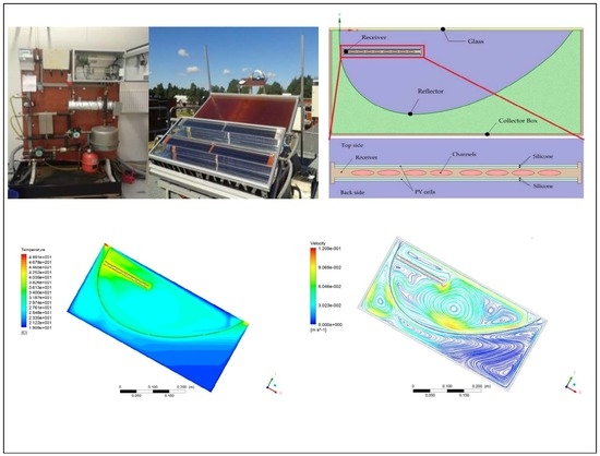
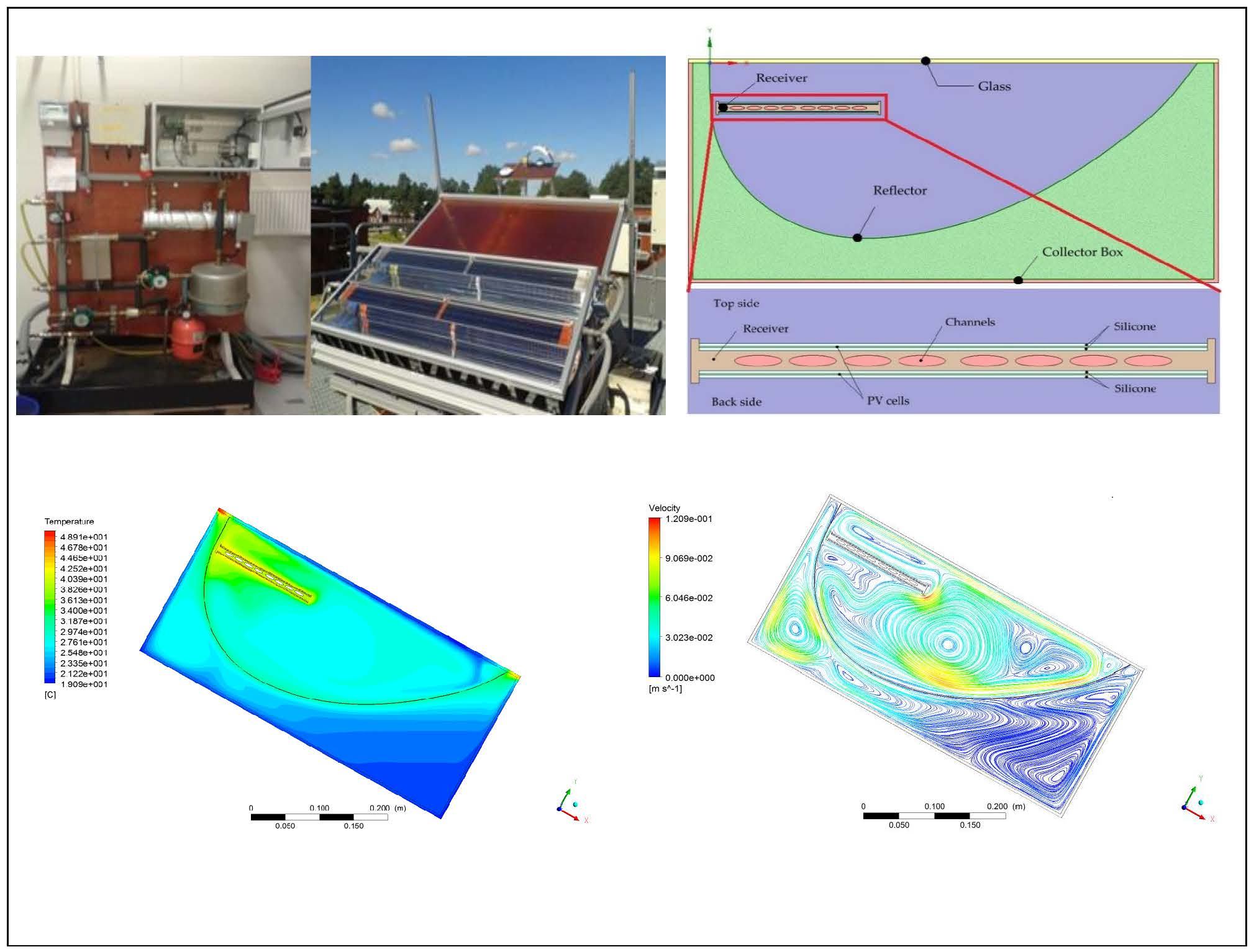
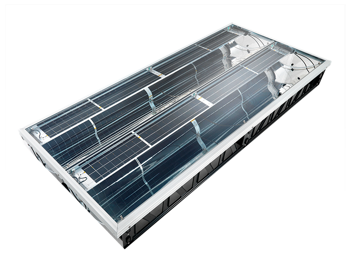
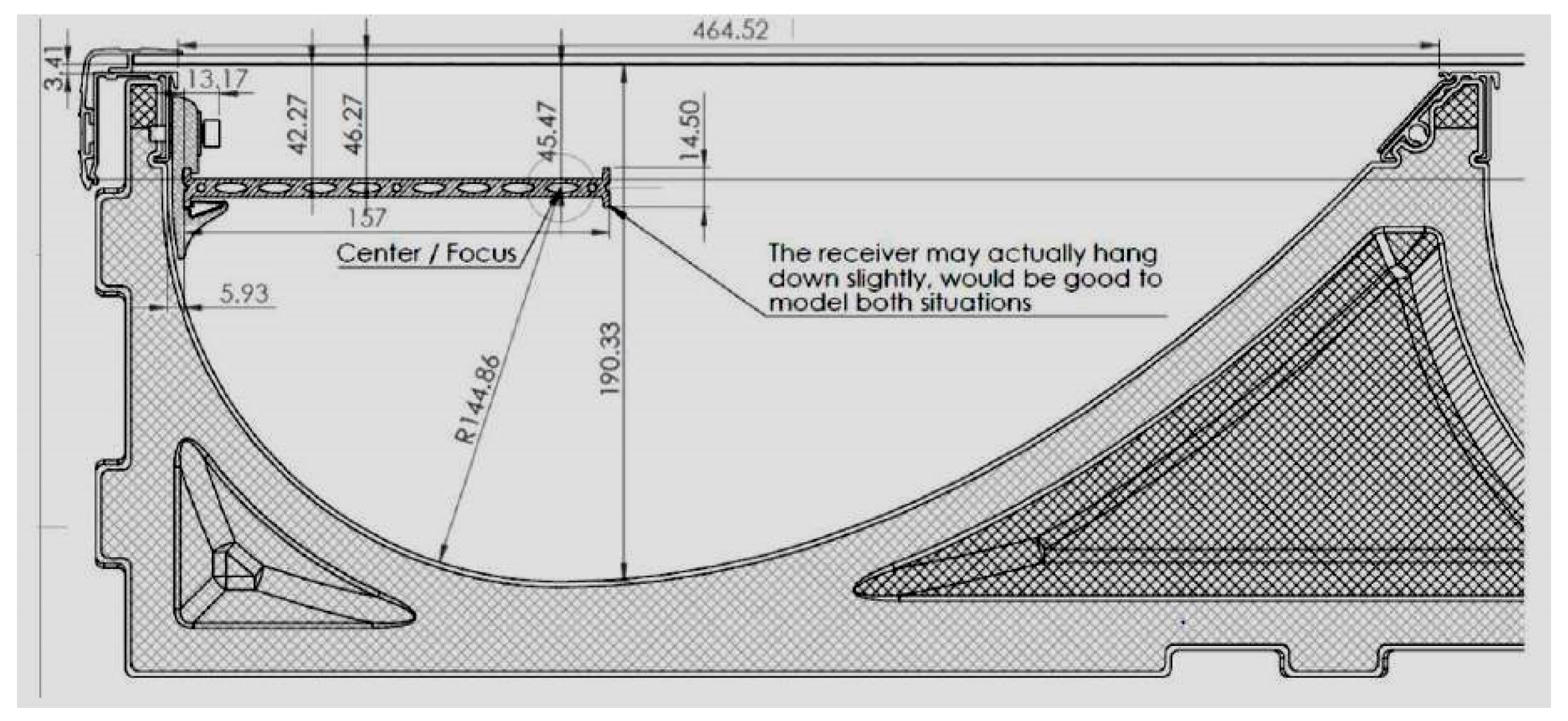
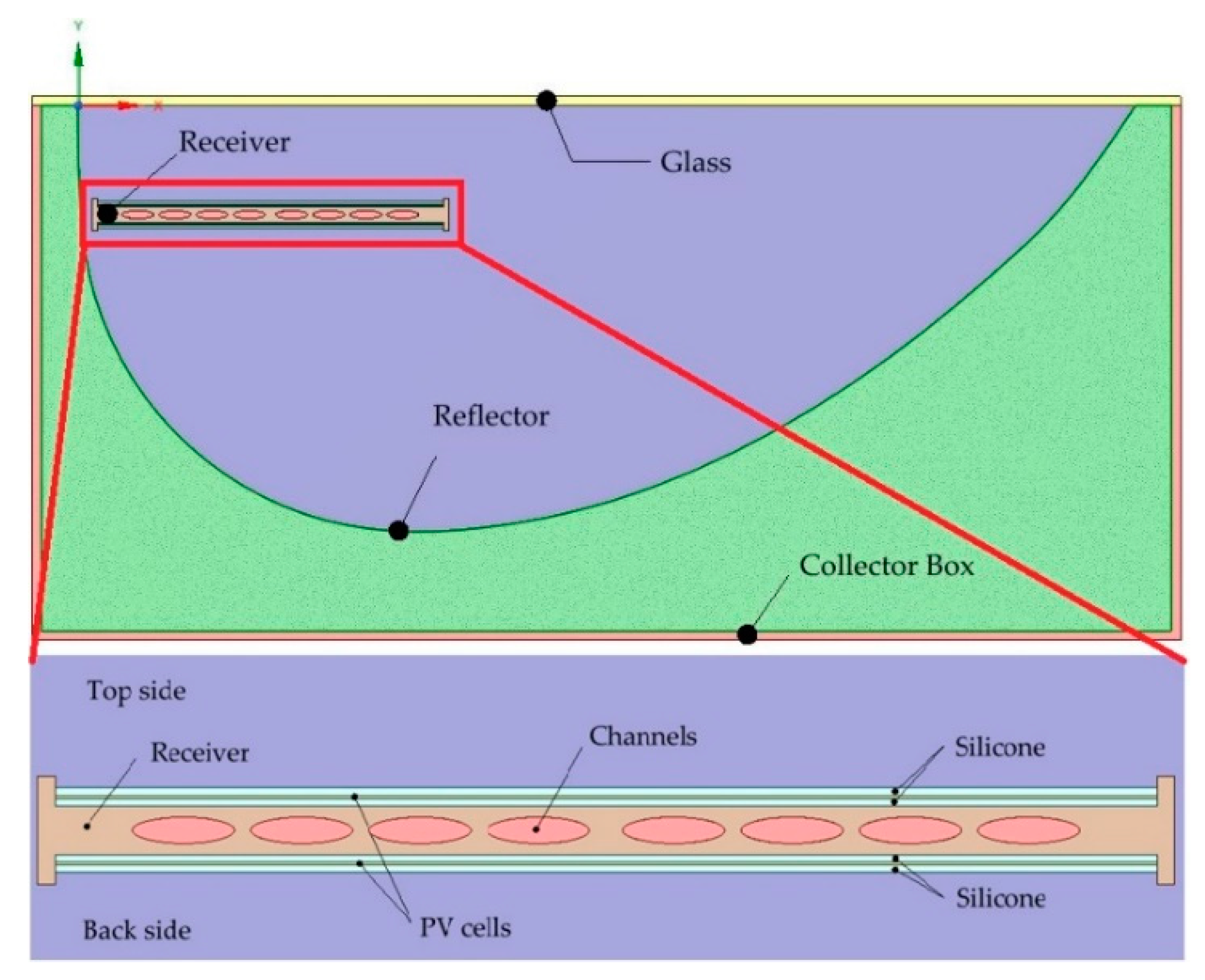
2.1. Description of the Collector and the Properties of its Components

Figure 1 shows the Solarus’s CPVT, which is called the PowerCollector. In Figure 1, it is possible to see the PV cell string layout on both sides (top side (facing the sky) and bottom side (facing the reflective material)) of the bifacial PVT receiver.

Figure 2 shows a schematic of the same collector from a top view [20]. The collector is 2.2 m² and it is divided into two troughs, each one with one receiver with 2.29 m of length and 0.158 m of width. It is characterized by an overall thermal efficiency of around 52% and the linear loss coefficient is 3.47W/(m² K) [21].

Reflector: Vattenfall AB has developed the reflector geometry of the collector, called Maximum Reflector Concentration (MaReCo). The reflector is a combination of a parabolic and circular reflective surface (commonly known as CPC reflectors) that concentrate the solar radiation onto the receiver. The details of the full geometry are described by Adsten et al. [22,23]. The reflective material has been selected from Almeco (VEGA125), with a total solar reflectance of around 96% for the full spectrum and 92% for the visible spectrum. The equation of the parabolic part of the reflector is (x² = y/0.0017), therefore the focal length is 144.86 mm (and circle radius). The focal point of the parabolic is located right on the center of the circle (Figure 3). Figure 4 shows how solar radiation is reflected to the receiver and PV cells.

Receiver: The receiver core is an aluminum extrusion with 8 elliptic channels. The PV cells are encapsulated with silicone on both sides of the receiver core.

Cell encapsulation and silicone: The PV cell encapsulation is done with two layers of silicone produced by Wacker. The encapsulation is done by pouring a bottom layer of 1 mm of silicone under the PV cells and a top layer of around 1 mm over the PV cells.

Standard Solar Cells: Each receiver side has two strings of 38 PV cells with an efficiency of 18.7% at Standard Test Conditions (STC) and connected in series. These PV cell series on both sides of the receiver are connected in parallel. The PV cell temperature coefficient was measured by Bernardo et al. and found to be 0.4%/C [24]. The PV cells have been cut, in order to be able to have dimensions of 52 by 148 mm. Overall, the collector has a total of 152 PV cells. The goal of cutting the cells is to lower the current, which is specifically important for concentrating collectors.

Glass: The solar glass is made out of low iron with a solar-weighted transmittance of 95% (stated by the producers, SunArc).

Table 2. The features of the PowerCollector.

Features	Values/Units
Collector production (nominal)	1350W thermal, 270W electrical
Collector total area	2.2 m2
Receiver area	0.362 m2
Concentration ratio	1.52
Reflector reflectivity	96% for the full spectrum and 92% for the visible spectrum
Receiver channel area	8 channels with 154 mm2 (one channel)
Silicone thickness	1 mm on both side of PV cells
Solar cell efficiency	18.7% (STC)
Solar cell Temperature coefficient	0.4%/C
Glass transmittance	95%

shows the features and details of the collector.

2.2. CFD Model of the Collector

Radiation, convection and conduction are the three ways of heat transfer that take place inside of the collector. The receiver and PV cells are heated by the sun’s radiation and then cooled by an HTF. The air inside of the collector starts moving due to the buoyancy-induced density gradient, creating free convection inside the collector. The physical behavior can be described by the continuity equation (Equation (1)), energy equation (Equation (2)) and the Navier Stokes equation (Equation (3)). These equations are Partial Differential Equations (PDE), nonlinear and coupled, therefore they need to be discretized and solved numerically [25].

$$\frac{\partial \mathsf{\rho }}{\partial \mathrm{t}}+\nabla ·\left(\mathsf{\rho }\mathrm{u}\right)=0$$

(1)

$${\mathsf{\rho }\mathrm{C}}_{\mathrm{p}}\left(\frac{\partial \mathrm{T}}{\partial \mathrm{t}}+\mathrm{u}·\nabla \mathrm{T}\right)+\nabla ·{\mathrm{q}}_{\mathrm{c}}=\mathrm{Q}$$

(2)

$$\frac{\partial \mathrm{u}}{\partial \mathrm{t}}+\left(\nabla ·\mathrm{u}\right)\mathrm{u}-\mathsf{\nu }{\nabla }^2\mathrm{u}=-\frac{1}{\mathsf{\rho }}\nabla \mathrm{P}+\mathrm{F}$$

(3)

where ρ is the fluid density, C_p is the specific heat constant, u is the fluid velocity, P is the fluid pressure, T is the fluid temperature and q_c can be defined by Fourier’s law—k∇T. Q and F are the heat generation and external forces, respectively.

2.2.1. Simulation Procedure

The CFD simulation has been developed by the finite volume method performed by ANSYS^® v2019 R3 fluent [26]. Firstly, the geometry of the collector was defined in the software and meshed optimally. Secondly, from the experimental results, the specific setup, variable and solution method were defined. Finally, the results of the model were analyzed and then compared with experimental results. The simulation model solved the continuity, energy and momentum equations inside the collector. Flow field, heat transfer, temperature gradient inside the receiver, thermal and electrical yield, and radiation field were obtained from these set of simulations.

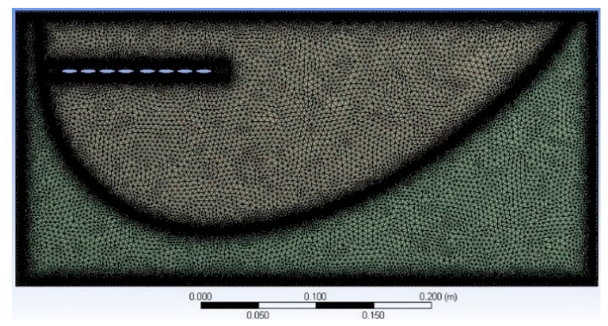
2.2.2. Geometry and Mesh of the Collector

A profile view (2D model) of the collector was used for the simulation (Figure 5). This geometry includes one trough of the collector, front box and detailed receiver with HTF channels, PV cells and silicone layers.

An air domain was defined inside the collector between the reflector, glass and receiver for the calculation of the fluid flow, free convection and radiation field. To simplify the geometry, some of the small parts of the collector were not considered. The 2D mesh was generated by ANSYS^® meshing tool (Figure 6). The collector has been meshed with a total number of 180,000 elements. The space around the receiver, the reflector and the surrounding edges were meshed carefully due to the strong temperature and velocity gradients.

2.2.3. Solution Methods

The simulation was performed in a pressure-based method and steady-state conditions, with the effect of gravity. The SIMPLE (Semi Implicit Method for Pressure Linked Equations) algorithm was used for pressure velocity coupling, first-order upwind discretization for the radiation, and a second-order upwind discretization for the momentum and energy. The simulations were performed by using the double-precision solver and standard under-relaxation factor. Body force weighted was used for pressure calculations. Due to the range of Rayleigh number (Ra = 10⁷), the laminar model was an excellent approximation to model the behavior of fluid inside the collector.

The PV cells produce electricity and reduce the total amount of heat transfer through the receiver. Then, a volumetric heat absorption was applied to the PV cells layer by using a UDF (User Defined Function) code. The efficiency of the PV cells was affected by their temperature. Therefore, the PV cells’ efficiency can be calculated by [4,27]:

$${\mathsf{ƞ}}_{\mathrm{cell}}\left(\mathrm{T}\right)={\mathsf{ƞ}}_0\left[1-{\mathsf{\beta }}_{\mathrm{PV}}\left({\mathrm{T}}_{\mathrm{PV}}-{\mathrm{T}}_0+{\Upsilon }_{\mathrm{G}}\log \left(\mathrm{G}\right)\right)\right]$$

(4)

β_PV is the temperature coefficient of the PV cell (0.4%/K for mono-crystalline cells) and is defined as the following:

$${\mathsf{\beta }}_{\mathrm{PV}}=\frac{1}{\mathrm{T}\prime -{\mathrm{T}}_0}$$

(5)

where T’ is the highest operating temperature of the PV cells, for which the efficiency drops to zero, T₀ is the standard temperature of 25 °C, and ƞ₀ is the efficiency of the PV cell operating at STC. ϒ_G is the intensity of the PV cell and in this condition, is set to zero because the effect of solar radiation on the PV cell is negligible. The electrical power output by the PV cells as the volumetric heat absorption is calculated by Equation (5), as can be seen below.

$$\mathrm{E}\left(\mathrm{T}\right)={\mathsf{ƞ}}_{\mathrm{cell}}\left(\mathrm{T}\right).\mathrm{G}.\frac{\mathrm{L}.\mathrm{W}}{{\mathrm{V}}_{\mathrm{cell}}}$$

(6)

where L.W are the dimensions (m), Vcell is the volume of the PV cell (m3) and G is the solar radiation (W/m2). This equation was applied as a UDF code for the PV cell in the model.

2.2.4. Material Parameter

Parameters such as materials, density, thermal conductivity, specific heat capacity and viscosity were considered independent from the temperature, except for the air. The air inside the collector was considered an incompressible ideal gas with a temperature-dependent density, as the free convection takes place inside the collector.

Table 3. Properties of different materials.

	Thermal Conductivity (W/m.K)	Density (kg/m3)	Specific Heat Capacity (J/kg.K)
Front Glass	1	2500	720
Reflector	200	2700	901
Receiver	210	2700	901
Silicon	0.2	970	1550
PV cell	124	2320	678
Collector Box	0.033	500	100

shows the properties of different materials.

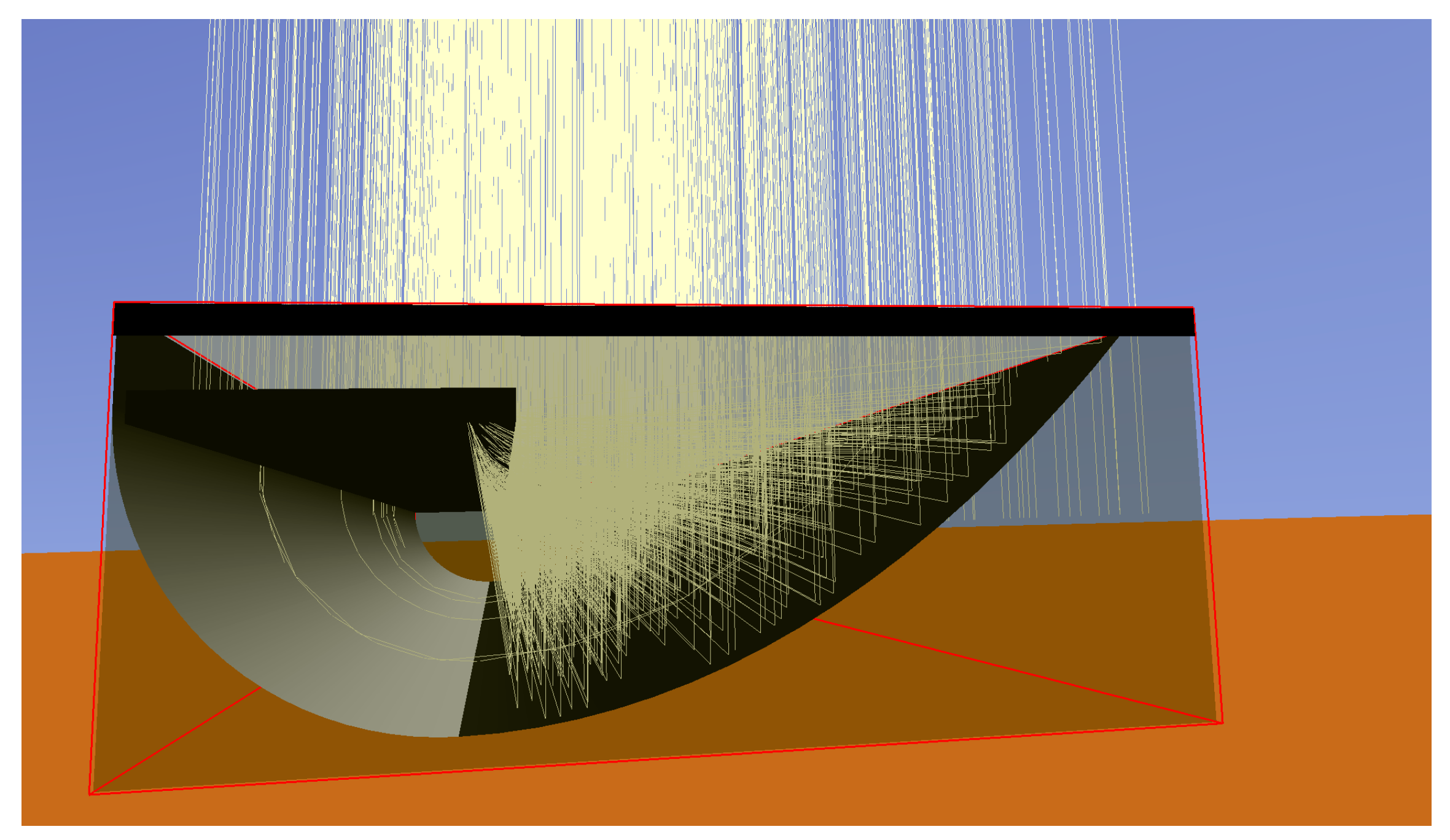
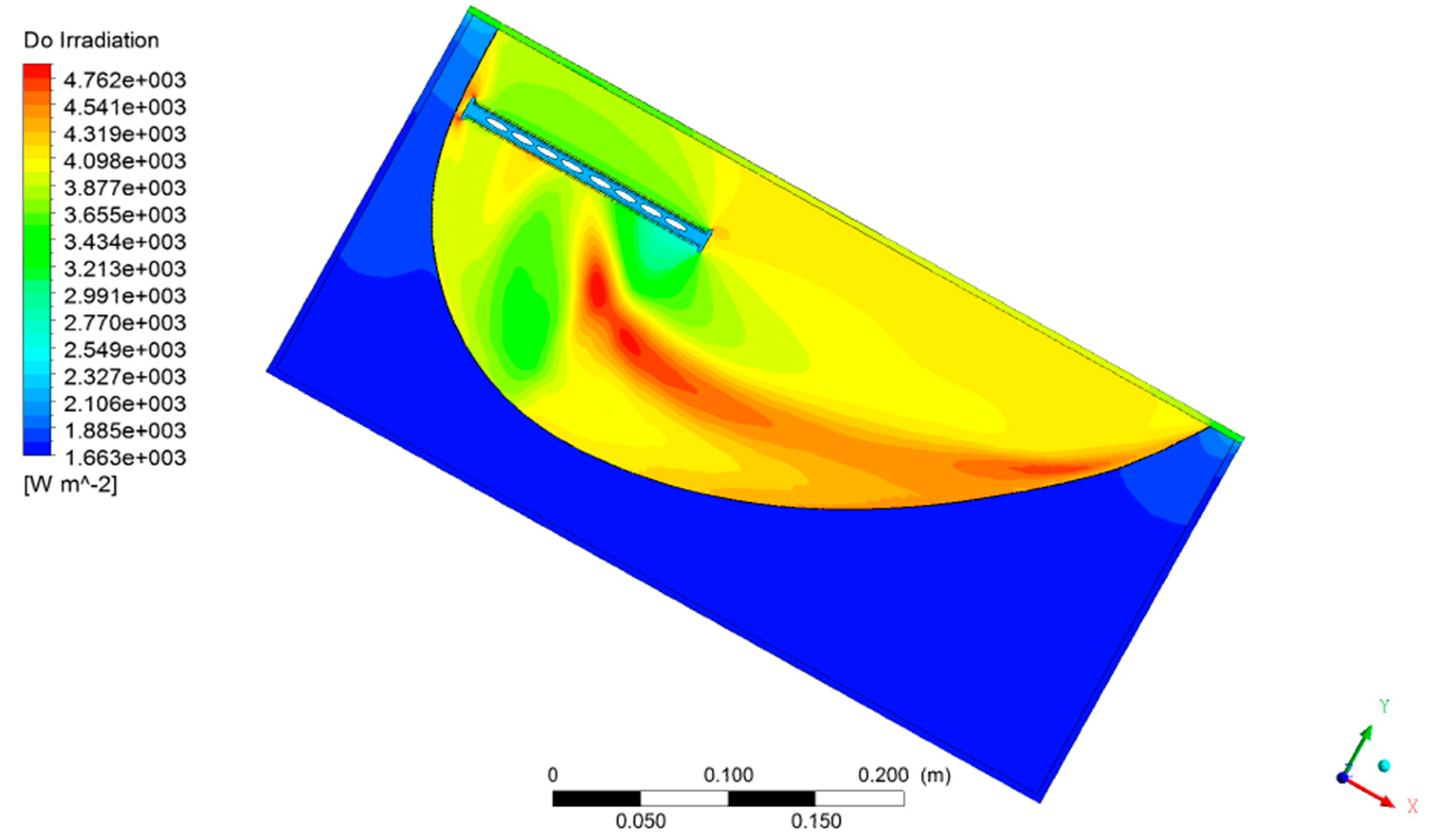
2.2.5. Radiation Model

To model the radiation field in the collector, the Radiative Transfer Equation (RTE) (Equation (6)) must be solved [28]:

$$\frac{\mathrm{dI}(\overrightarrow{\mathrm{r}}.\overrightarrow{\mathrm{s}})}{\mathrm{ds}}+\left(\mathsf{\kappa }+{\mathsf{\sigma }}_{\mathrm{s}}\right).\mathrm{I}(\overrightarrow{\mathrm{r}}.\overrightarrow{\mathrm{s}})= \mathsf{\kappa }.{\mathrm{n}}^2.\frac{\mathsf{\sigma }.{\mathrm{T}}^4}{\mathsf{\pi }}+\frac{{\mathsf{\sigma }}_{\mathrm{s}}}{4\mathsf{\pi }}.{{\displaystyle \int }}_0^{4\mathsf{\pi }}\mathrm{I}(\overrightarrow{\mathrm{r}}.\overrightarrow{\mathrm{s}}).\mathsf{\Phi }\left(\overrightarrow{\mathrm{s}}.\overrightarrow{\mathrm{s}}\prime \right)\mathrm{d}\mathsf{\Omega }$$

(7)

where r and s are the position and direction vectors, I is the radiation intensity, n is the refraction index, σ is the Stefan–Boltzmann constant (5.67 × 10^-8 W/m2.K4), and σ_s and κ are the scattering and absorption coefficients, respectively. T is the local temperature and Φ is the scattering phase function that describes the probability that a ray from one direction (s) will be scattered into a certain direction (s’). The numerical method used to solve the RTE equation was the Discrete Ordinate Method (DOM), as this model allows a specular surface to be defined. This method solves the radiation field inside the model for a finite number of discrete solid angle and direction vectors. The DOM method requires a directional discretization and, to avoid the ray effect, an angular discretization of 15 × 15 divisions (Theta divisions and Phi division) and 3 × 3 pixels (Theta pixels and Phi pixels) was specified [29]. All the surfaces were set as opaque with diffuse reflectivity, except for the glass and reflector. The glass was set as a semi-transparent surface and the reflector was set as a specular surface. The absorption and scattering coefficient were not considered for the air.

2.2.6. Boundary Conditions

Different categories of boundary conditions were defined. The forced convection heat transfer coefficient with an average temperature was used to model the fluid channels. From the experimental results, the average value for HTF was found. The heat transfer in the HTF domain was not solved. The heat transfer coefficient inside the channels is a function of the Nusselt number (Nu_d), the thermal conductivity of the fluid (k_f) and the hydraulic diameter (D_h), and is defined as [25]:

$${\mathrm{h}}_{\mathrm{w}.\mathrm{forced}}=\frac{{\mathrm{Nu}}_{\mathrm{d}}{\mathrm{k}}_{\mathrm{f}}}{{\mathrm{D}}_{\mathrm{h}}}$$

(8)

Reynolds calculations showed that the flow regime inside the channels was laminar. Because of the high thermal conductivity of the receiver, the temperature of the channels was uniform. Then, the Nusselt number was constant Nu_d = 3.66 [25]. The thermal generation of the collector is calculated by Equation (8), where h_w,forced is the heat transfer coefficient, T_f is fluid temperature and T_w is the temperature of the channels.

$${\mathrm{Q}}_{\mathrm{th}}={\mathrm{Ah}}_{\mathrm{w}.\mathrm{forced}}\left({\mathrm{T}}_{\mathrm{f}}-{\mathrm{T}}_{\mathrm{w}}\right)$$

(9)

The glass cover was modeled as a semi-transparent surface with an emissivity of 0.95 and with a thickness of 4 mm. The solar glass is made out of the iron glass with a solar weighted transmittance of 95%. Solar beam and diffuse radiation were defined according to the experimental measurements and solar angles were calculated using the setup place coordinates. The glass has a radiative heat loss to the sky (T_sky) and a forced convective heat loss to the ambient because of wind (T_amb). The heat transfer coefficient caused by wind and sky temperature is calculated as described by Kalogirou [4]:

$${\mathrm{h}}_{\mathrm{wind}}=\frac{8.6 .{\mathrm{V}}^{0.6}}{{\mathrm{L}}^{0.4}}$$

(10)

$${\mathrm{T}}_{\mathrm{sky}}=0.0552{\mathrm{T}}_{\mathrm{amb}}^{1.5}$$

(11)

where V is the wind speed (m/s) and L is the characteristic length of the collector (m). The average wind speed in the model was set to 3.14 m/s and the characteristic length was set to 2.31 m.

The receiver is made out of aluminum with an emissivity of 0.4. The PV cells have 0.4 mm thickness and are placed between two-silicone layers with 1 mm thickness. The boundary conditions of the PV cells and silicone were the conjugated wall because of conduction heat transfer between them. The temperature of these layers was analyzed and later on compared with the experimental data retrieved from the outdoor tests. The reflector was modeled with a specular surface (ϵ=0.05) with a 96% reflectivity and a 0.4 mm thickness. On the other hand, the backside of the reflector has been modeled as a diffuse surface (ϵ=0.3).

The collector box is made out of polycarbonate (ϵ=0.95) with a thickness of around 4 mm. It is exposed to the surrounding area and has a convective heat loss to the ambient. A forced convection heat transfer coefficient (h_wind) with ambient temperature was defined for the collector box boundary conditions.

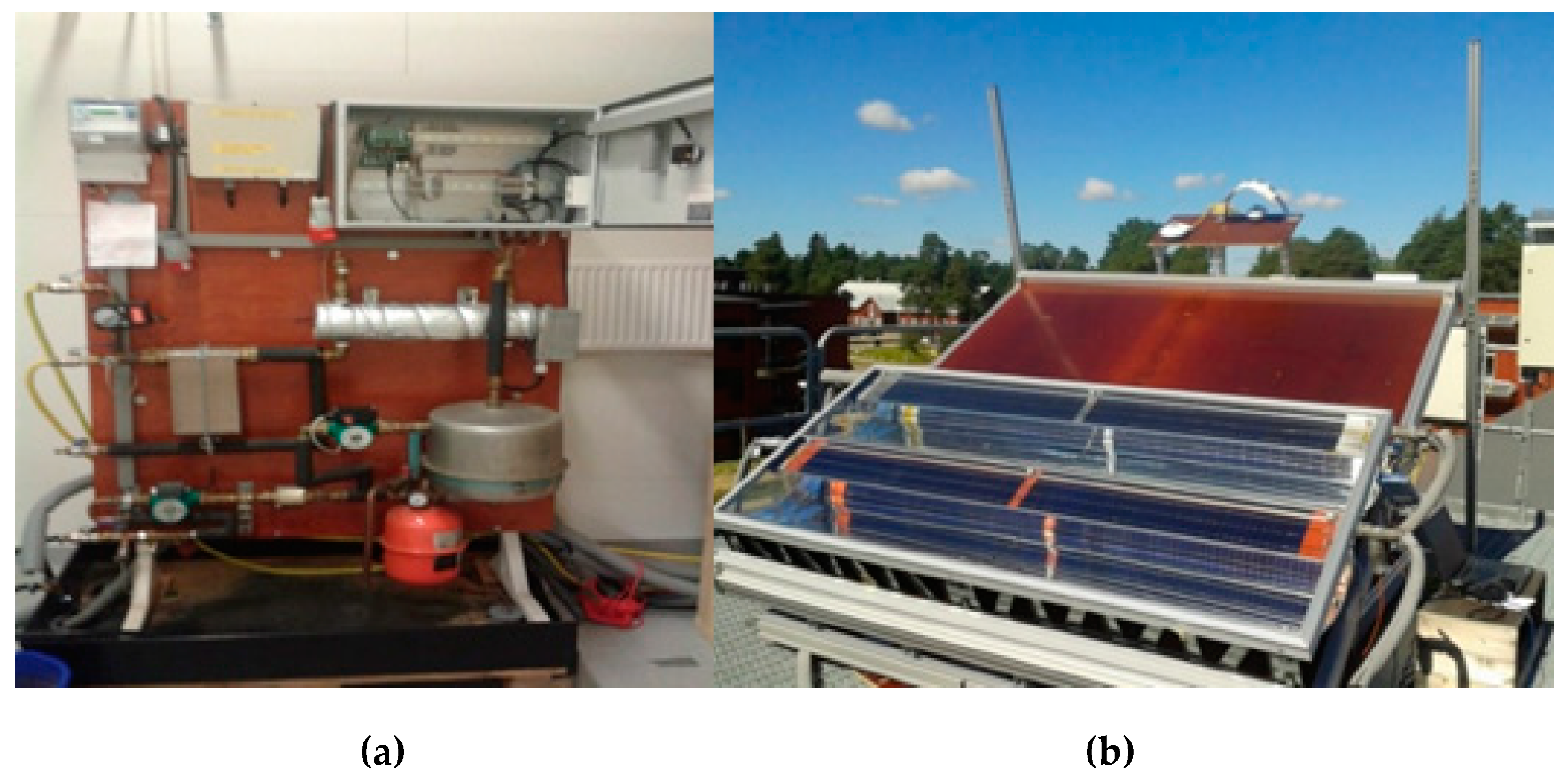
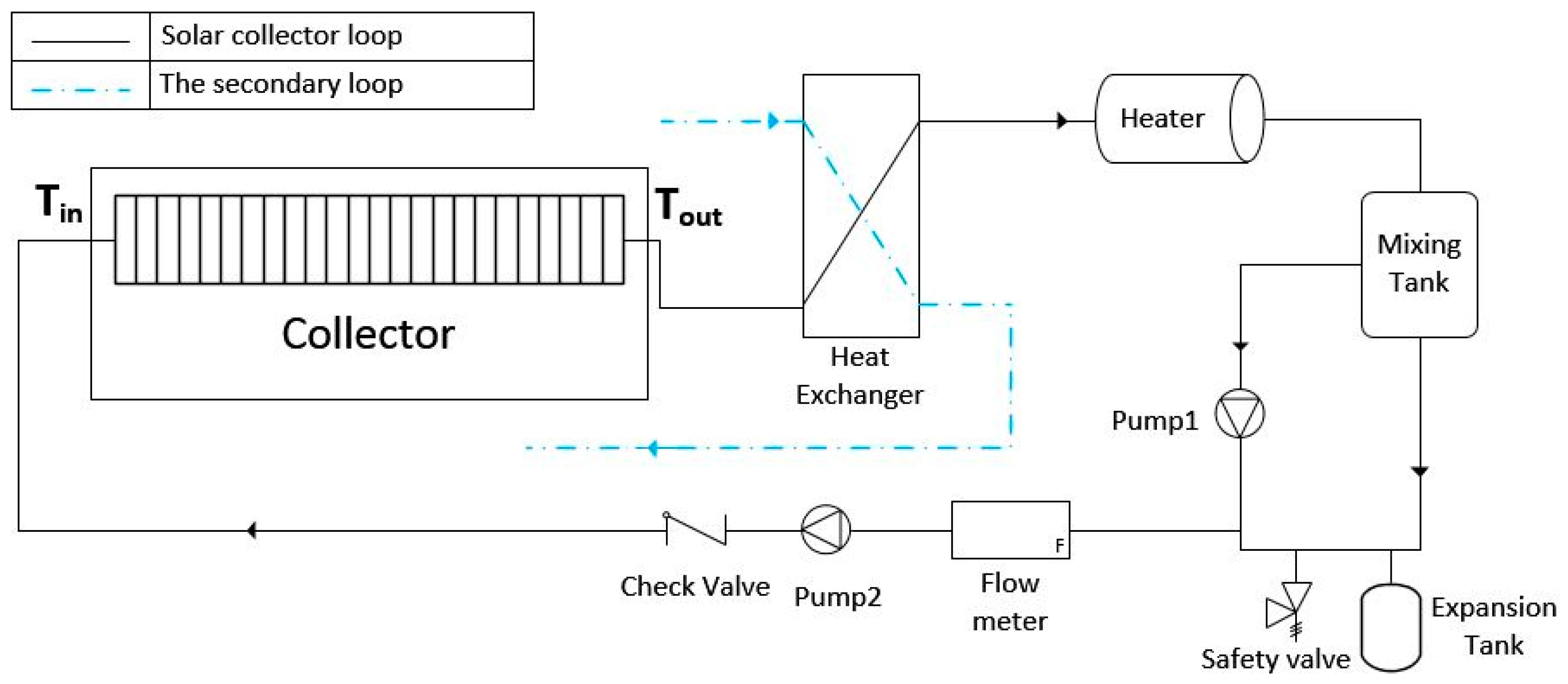
2.3. Experimental Test Method and Equipment Description

Figure 7 describes the experimental setup. The setup consists of temperature, flow and radiation measurements. The collector has been installed in the outdoor testing laboratory (coordinates: 60°N; 17°E) at Gävle University, with a surface tilt angle (β) of 30° (south-oriented).

Figure 8 shows a schematic of the experimental setup. The setup consists of two loops: a solar collector loop (closed loop) and a secondary loop (open loop). The solar collector loop relates to the HTF flowing between the collector and heat exchanger, supplied by a fixed flow by pump 2. Furthermore, on the solar loop, measurement equipment has been installed in order to measure the system operation, and these are presented below.

• KippZonen CMP3 and CMP6 pyrometers were used to measure solar direct and diffuse radiation.
• PT100 thermal resistances were used to measure the inlet and outlet fluid temperature and ambient temperature.
• K-type thermocouples were used for measuring the PV cells’ temperature.
• 2 Omega FMG80 flowmeters were used to measure the flow rate in each trough.
• A PicoLog USB TC08 datalogger was used to collect the data from the K-type thermocouples.
• A datalogger CR1000 from Campbell Scientific was used to visualize/store the parameters obtained by the PT100 ambient and water flow temperature sensors, the CMP3 and CMP6, and flowmeters.

The secondary loop relates to the outlet water from the heat exchanger. The heater and mixing tank were used to have a different value of HTF temperature. Whenever the heater is working, pump 1 recirculates the fluid, in order to achieve a uniform temperature.

Six measurements (A, B, C, D, E and F) were taken on three different dates and times. Measurements A and B on day one (August 17), C and D on day two (August 18) and E and F on day three (August 25) were conducted. The stagnation test was conducted on measurement F, where no HTF flow rate has been implemented and the heat losses were equal to the energy received from the sun [20]. For each measurement, the inlet and outlet water temperature for one trough of the collector, ambient temperature, solar beam and diffuse radiation, and temperature of different layers of the collector were measured (

Table 4. Different parameters of each measurement.

Measurement	Ambient Temperature (°C)	Inlet Water Temperature (°C)	Outlet Water Temperature (°C)	Direct Radiation (W/m2)	Diffuse Radiation (W/m2)	Incident Angle (⁰)	Solar Altitude(⁰)	Solar Azimuth (⁰)	Flow Rate (L/min)	Duration of Measurement (min)
A	18.6	33.6	36.6	978.3	93.1	18.5	48.5	199.4	2.2	10
B	19.1	42.9	46.2	922.8	77.2	26.4	56.3	231.9	1	5
C	20.1	46.3	48.4	946.0	77.2	17.9	47.8	189.4	2.2	10
D	20.8	44.7	47.5	892.9	76.4	28.1	58.1	235.7	1.2	5
E	21.6	36.2	39.0	757.8	145.5	21.4	51.4	200.9	2.1	3
F	23.1	-	-	422.5	114.6	29.2	59.2	231.8	0	3

). Table 4 shows the average values for each parameter. The incident angle is the angle between the sun’s rays and the normal on the surface of the collector.

Four K-type sensors (1, 2, 3 and 4) were located as described in Figure 9. Each K-Type sensor was soldered on a different part of the receiver. The K-type temperature sensors have been numbered according to the list below.

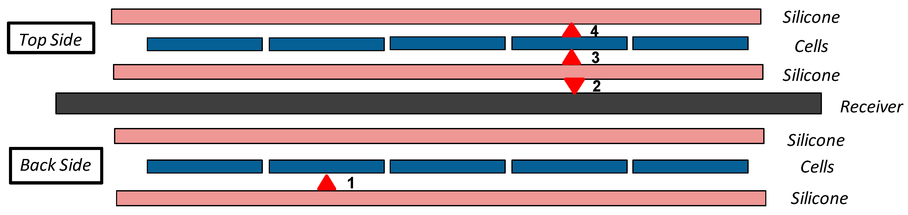
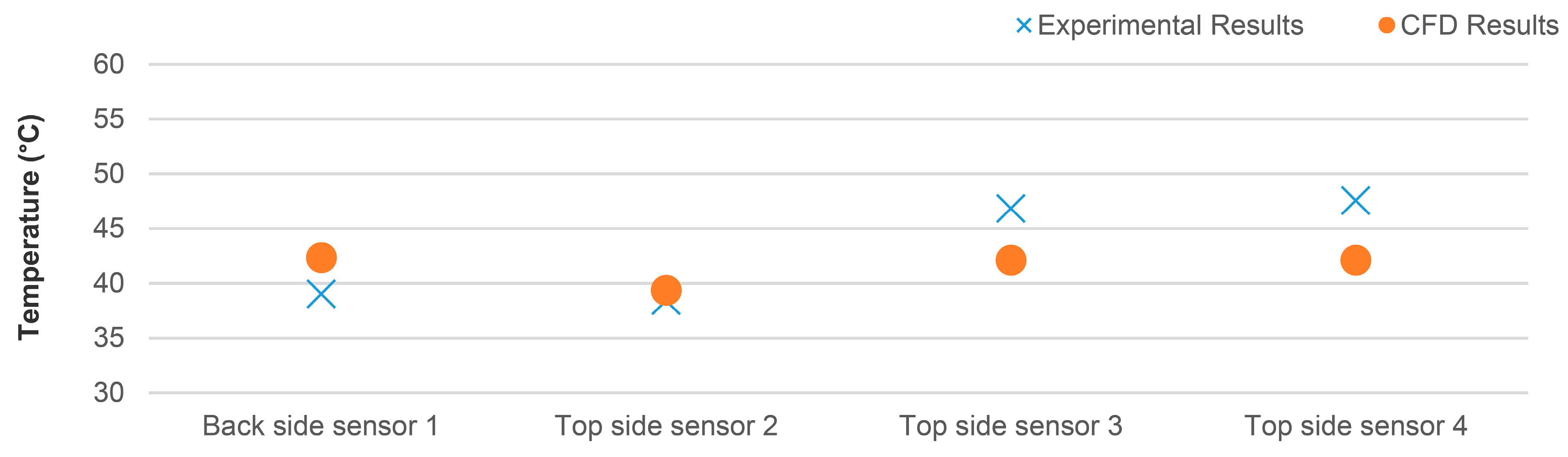
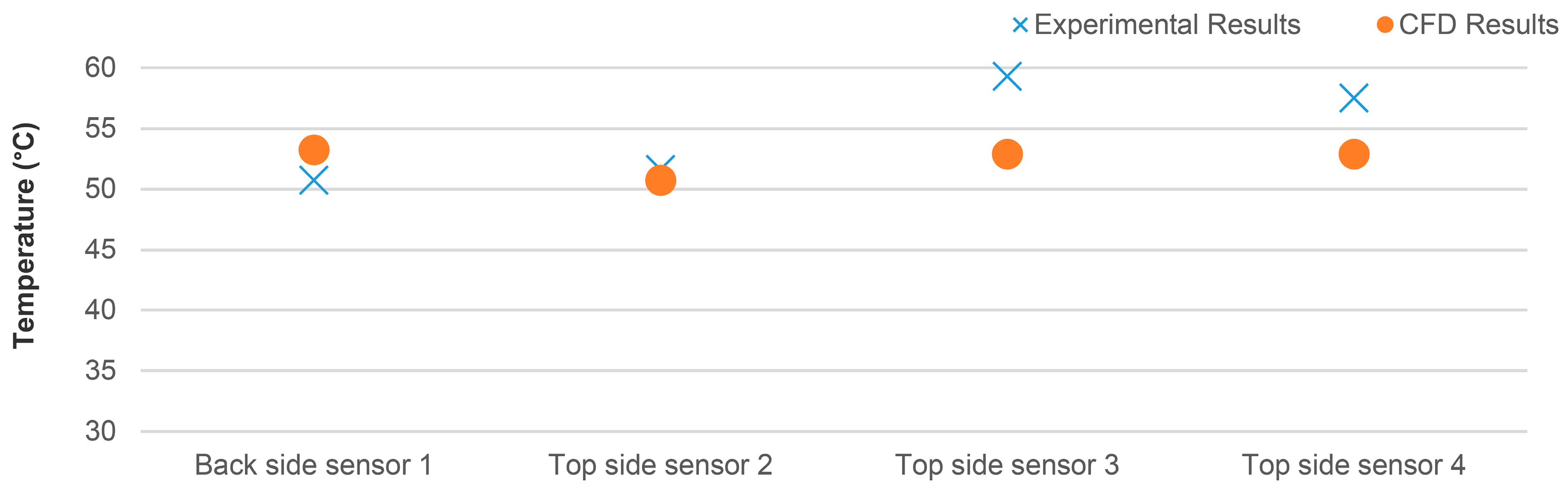
• Back side sensor 1: Temperature over the cell (second cell).
• Top side sensor 2: Temperature on the receiver (fourth cell).
• Top side sensor 3: Temperature under the cell (fourth cell).
• Top side sensor 4: Temperature over the cell (fourth cell).

3. Results and Discussion

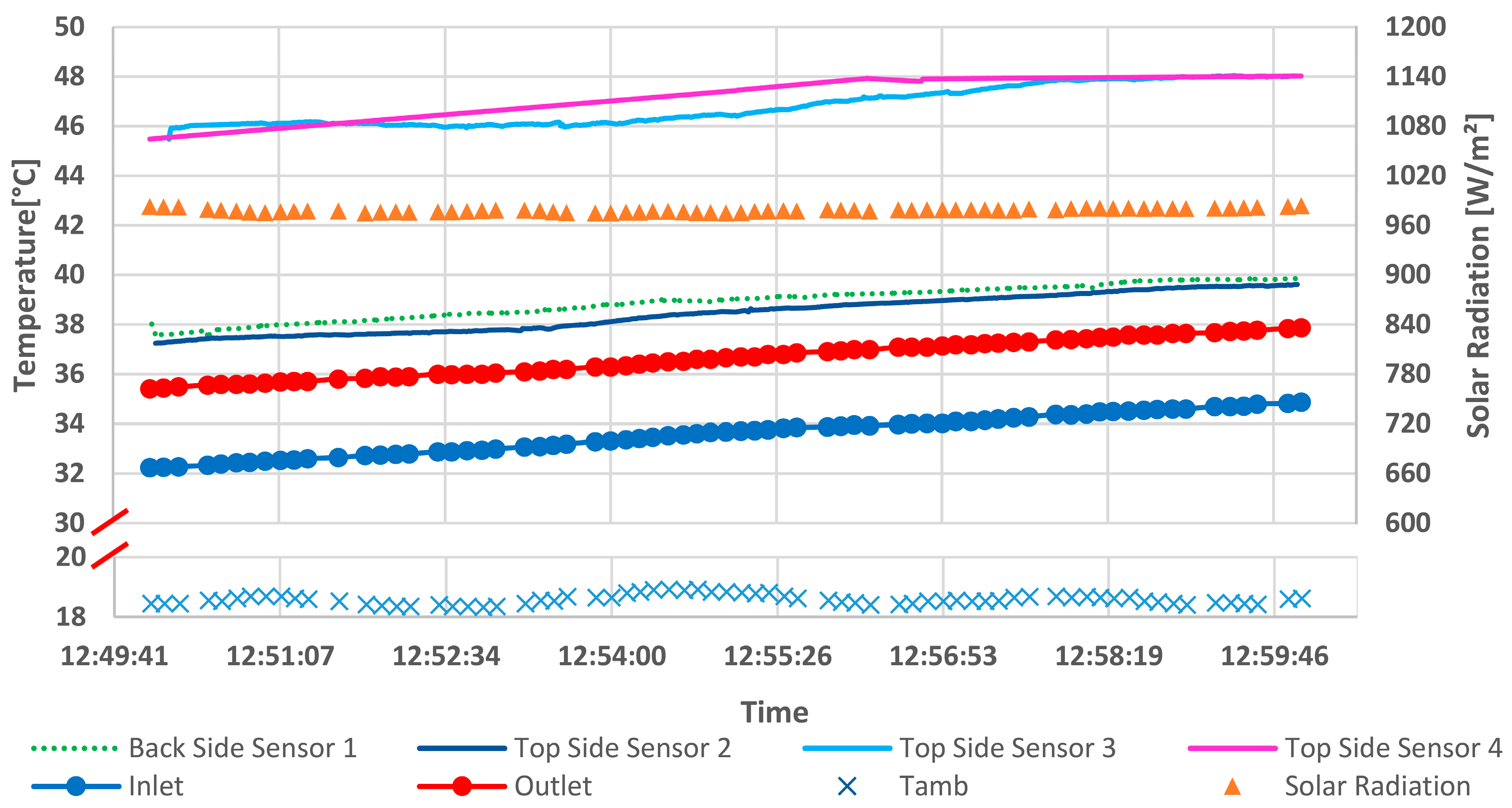
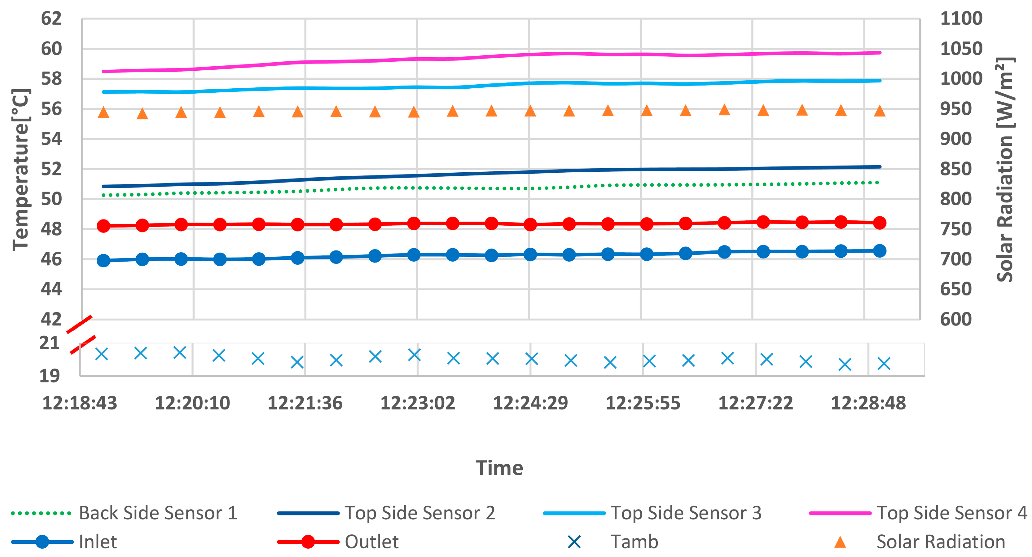
3.1. Experimental Results

In this section, experimental results are presented and analyzed. Figure 10, Figure 11 and Figure 12 show the temperature of different layers of the receiver, ambient temperature, inlet and outlet water temperatures, and solar radiation for measurements A and B. Top side sensor 2 shows a value close to the HTF temperature, showing a good thermal conductivity. Solar radiation is focused on the back side of the receiver with the highest temperature on the focal point. In these measurements, back side sensor 1 was located far from the focal point (as the focal point is set by the reflector’s specific geometry and sun’s relative position). Therefore, it shows a temperature close to the HTF. On the other hand, top side sensors 3 and 4 show nearly the same values due to the high thermal conductivity over the very thin PV cells (124W/m.K). Back side sensor 1 would be expected to show the highest temperature value located, but as the sensor is not under the focal point, this does not happen.

3.2. Validation of the CFD Model

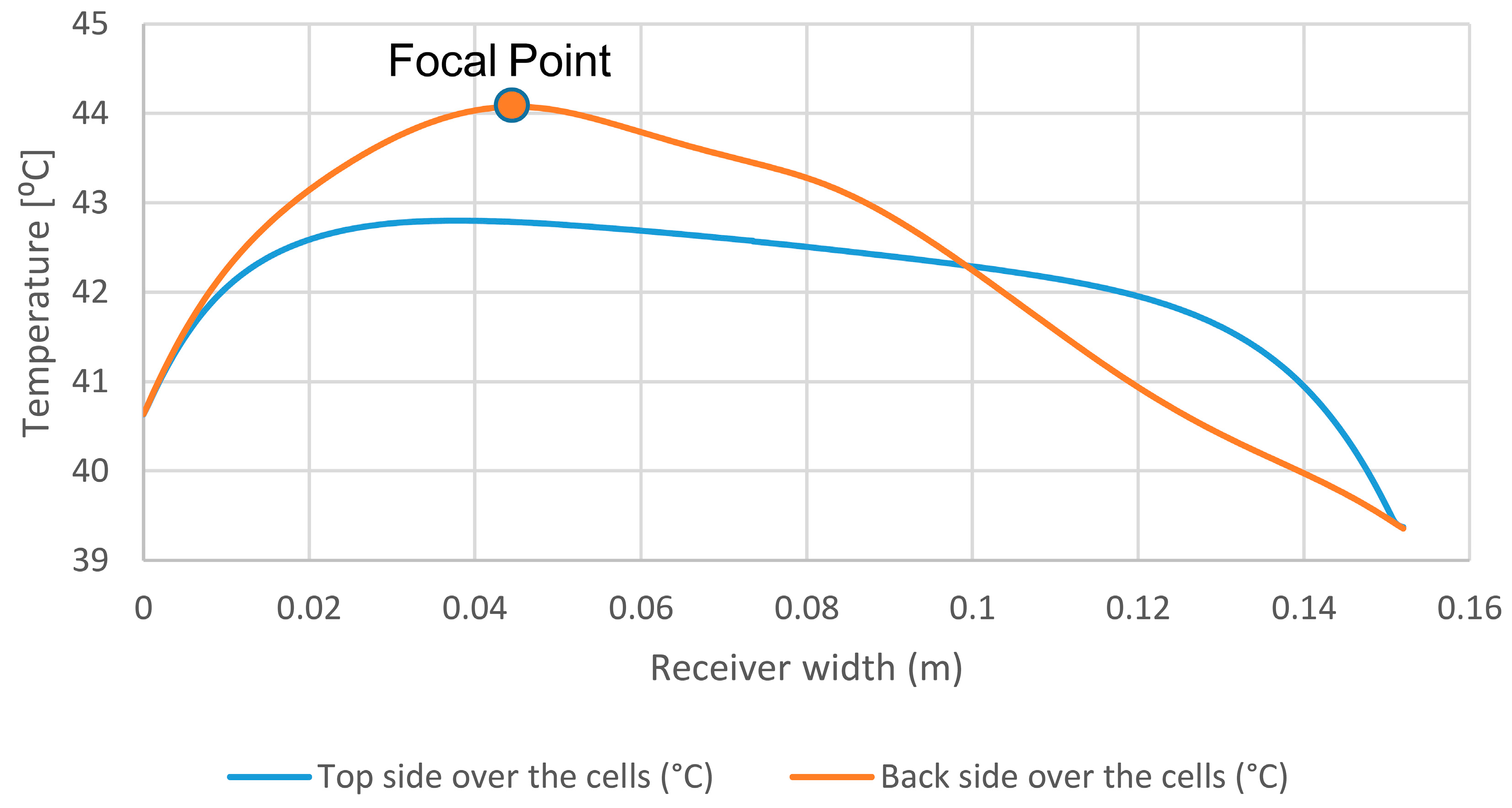
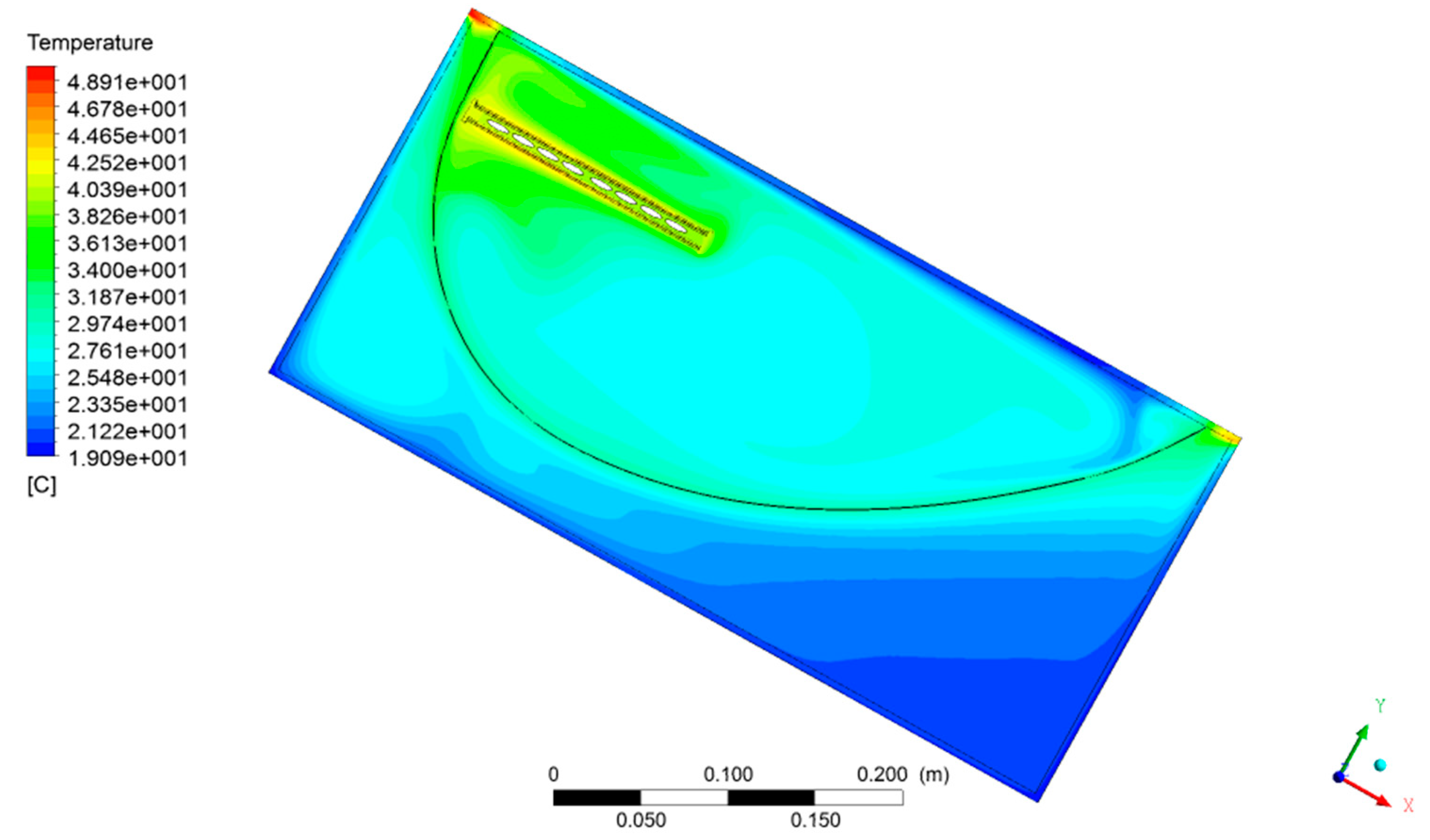
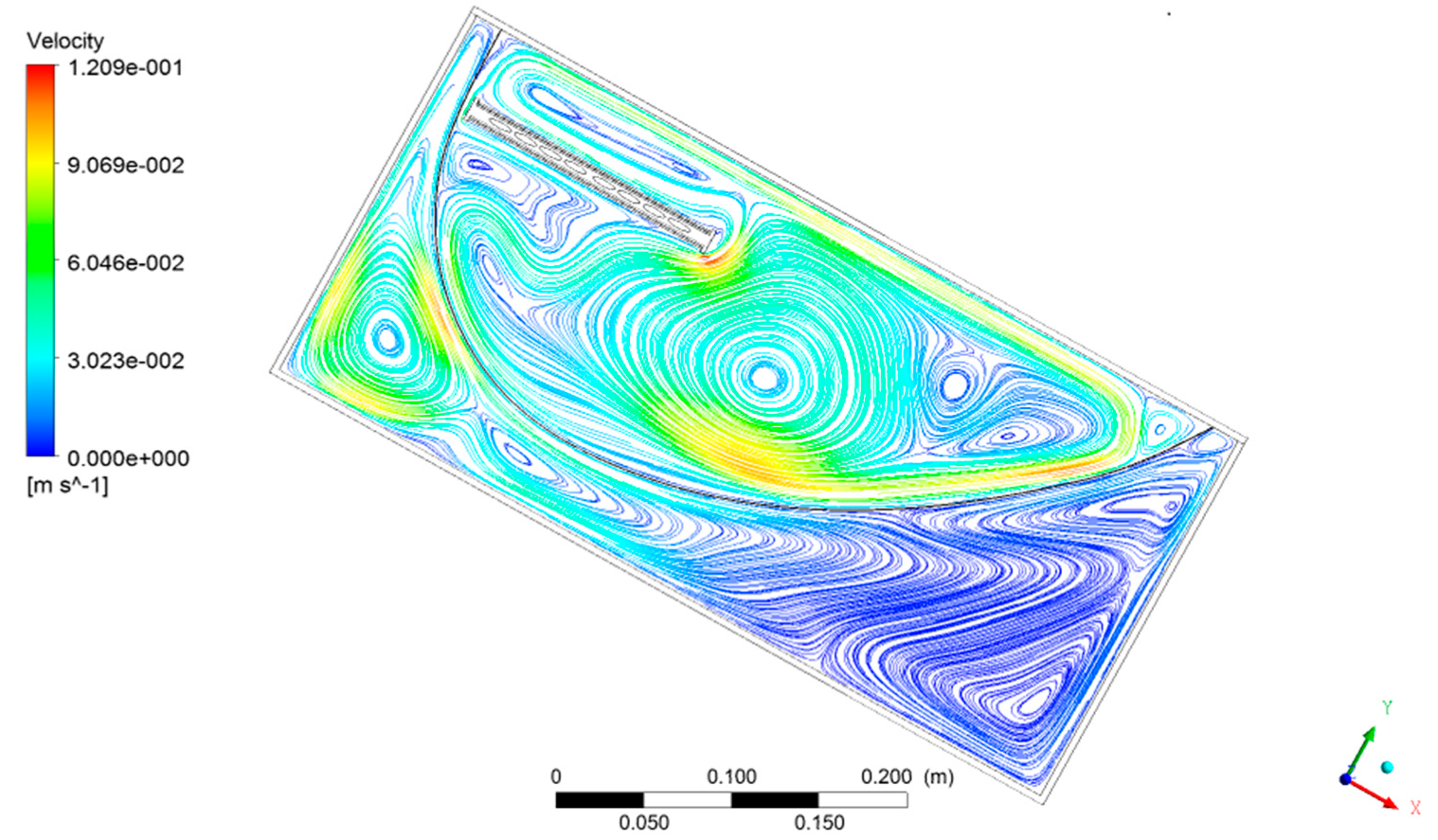
In this section, the CFD model is validated with experimental results. Figure 13 shows the CFD results for a temperature distribution over the cells on both sides of the receiver (outer part) for the conditions of measurement A. This Figure shows that the back side of the receiver (where the focal point is located) can reach the highest temperature and sensor 1 can show this temperature if it is under the focal line. The top side of the receiver has a flat distribution due to the uniform solar radiation (no focal line). Both ends of the receiver have the same value, which is lower than other parts of the receiver due to the convection heat transfer from the receiver to the air inside the collector. Figure 13 also shows that the placement of the sensor 1 on the back side of the receiver is important because the PV cells might reach a ΔT of around 5 °C (44 to 39 °C) along the receiver width. This accounts for the back side sensor 1 showing lower temperatures than the top side sensor 4.

Figure 14, Figure 15 and Figure 16 show the comparison between experimental and CFD results. The temperature of different layers of the receiver from experimental results were compared with the CFD results for measurements A, B and C. The experimental results are average values during the measuring time and CFD results are weighted average values along with the receiver (according to the temperature distribution).

Figure 14, Figure 15 and Figure 16 show a reasonable fit between the experimental and the CFD results, as the deviation from the CFD model varies from 0.2% up to 11.4%. The average deviation value for four sensors is 7%.

3.3. CFD Results

The validation of the model allows further analysis of the CFD results. Figure 17 shows the distribution of incident total radiation in the collector for a tilt angle of 30°, as in measurement A, where the temperature of different layers of the receiver, ambient temperature, solar radiation and flow rate was measured. The reference case is the only measurement A. Several parameters were changed to study their impact on the collector performance and compared with the reference case. The parameters were collector tilt angle, different HTF temperature, no front glass, receiver material and insulation. Figure 17 shows how solar radiation is focused on the back side of the receiver.

Figure 18 and Figure 19 show the distribution of temperature and velocity streamlines inside the collector for measurement A, respectively. Figure 18 shows that the hottest part of the collector is, as expected, the receiver, due to the high absorbance of light by the solar cells and the concentration. The bottom of the collector and front glass have the lowest temperature because of convection heat transfer to the ambient.

Figure 19 shows how the air moves inside the collector (an eddy movement). The air on both sides of the receiver gets hot, and due to the temperature-dependent density, travels upwards. Then, it moves under the front glass, and it’s temperature reduces because of heat losses to the ambient and goes down. The reflector absorbs a small fraction (4%) of solar radiation and gets hot then increases air temperature. The air goes upward and this circulation is repeated. In the collector box (under the reflector), the air warms up and goes up. The walls of the collector’s box show convective heat loss to the ambient. Therefore, the air temperature decreases and the air moves down.

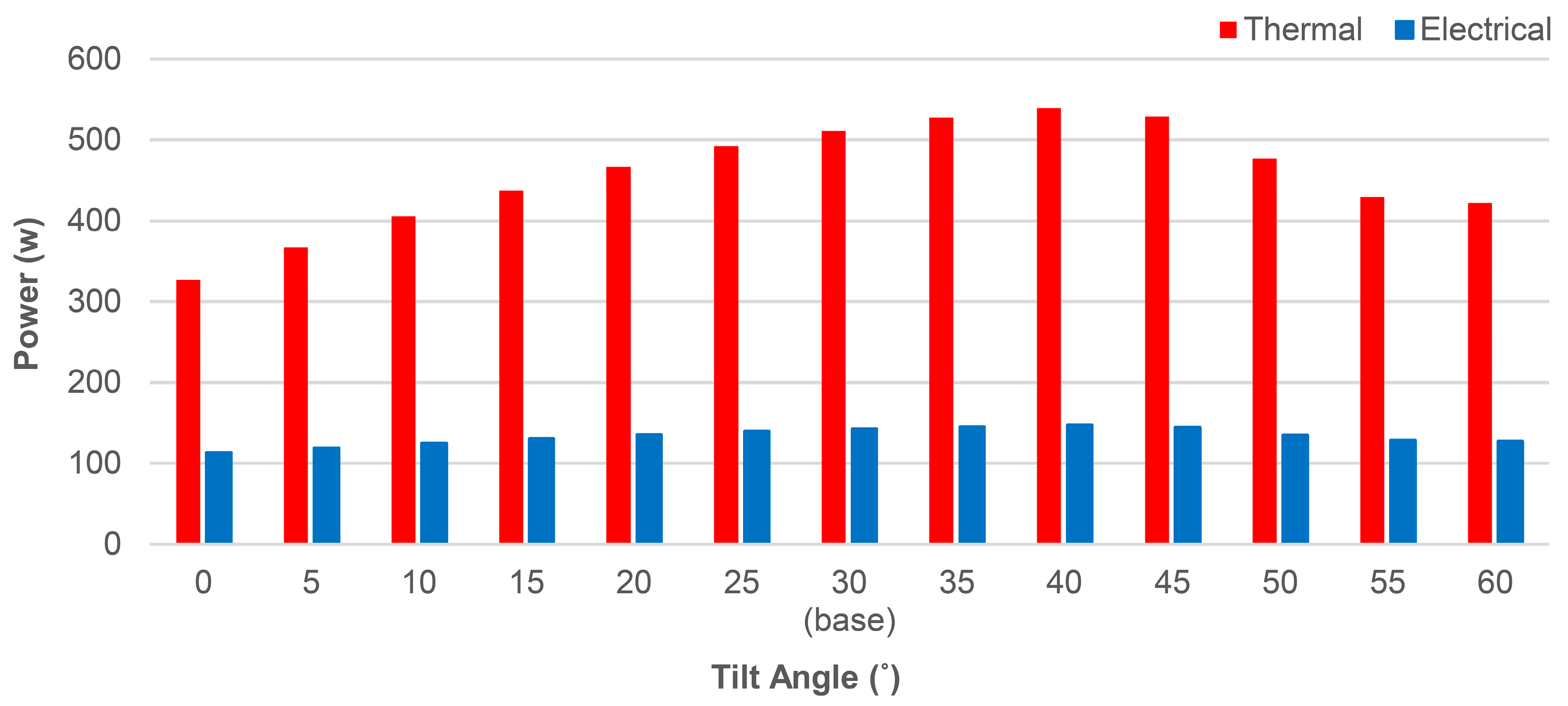
3.3.1. Collector Tilt Angle Variation

The collector tilt angle has been varied between 0° and 60° under the condition of measurement A (Table 4) to study the effect of tilt angle on the electrical and thermal productions of the collector. In Figure 20, the thermal and electrical power of the collector at different tilt angles is shown for a specific time of the year. For a 40° tilt angle, the incident angle is 8.5° and the thermal and electrical power reaches the maximum values of 539 W and 147 W, respectively. It should be mentioned that this is not the optimum angle of installation for the collector for the whole year and just shows the effect of tilt angle on the collector productions. It also shows that the effect of tilt angle on thermal production is more serious than the electrical one.

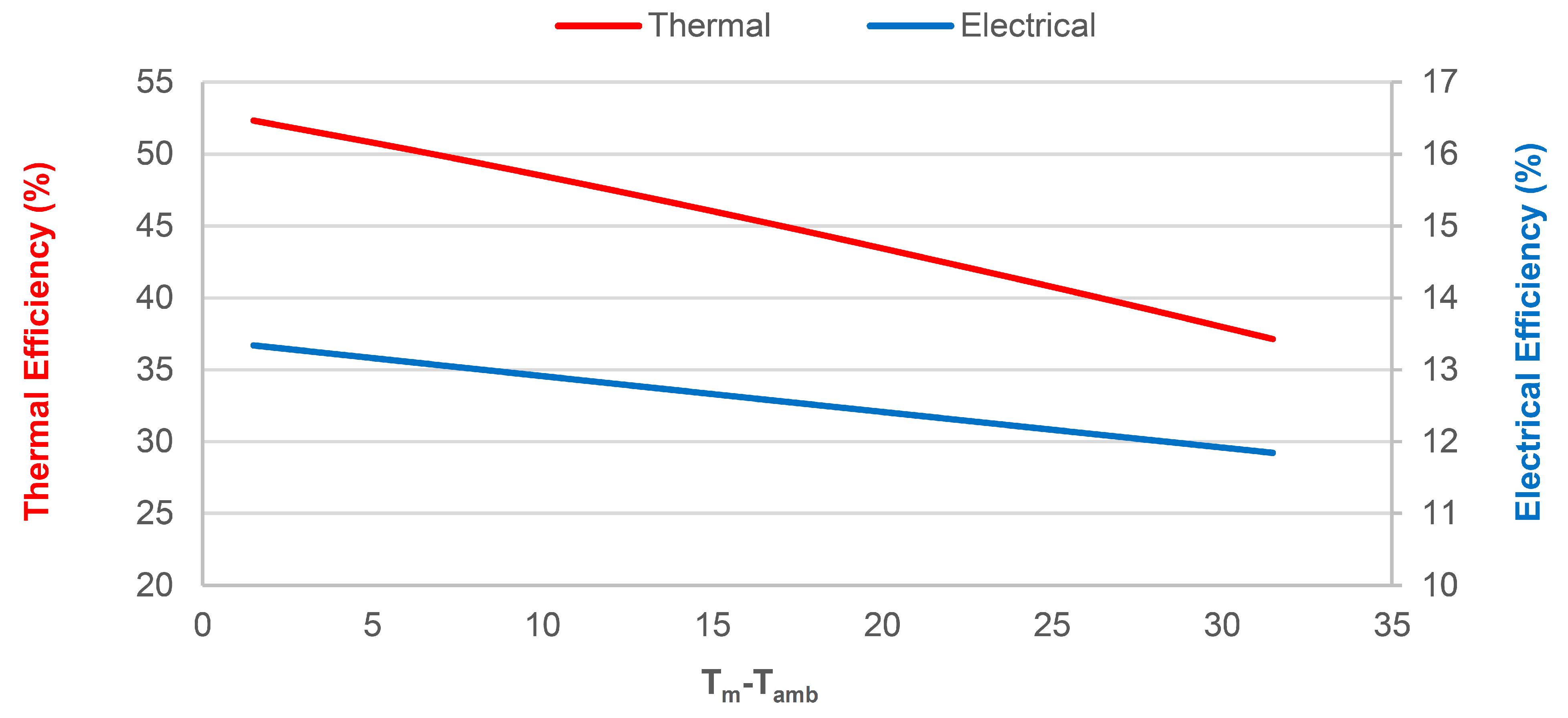
3.3.2. HTF Temperature Variation

Different HTF temperatures were modeled and are presented in Figure 21. Figure 21 shows the performance of the collector versus ΔT (T_m-T_amb). T_m is mean HTF temperature and T_amb is the ambient temperature. At higher HTF temperature, the thermal efficiency of the collector decreases and that is due to the decreasing temperature gradient between the receiver and HTF.

Figure 21 shows that the slope of thermal efficiency line and Equation (12) [4] is (U/G = 0.005) and solar radiation for measurement A is 978.3W/m². The collector heat loss coefficient (U) is calculated as 4.89 W/m².K.

$$\mathsf{ƞ}={\mathsf{ƞ}}_0-\frac{\mathrm{U}.\Delta \mathrm{T}}{\mathrm{G}}$$

(12)

Figure 21 also shows that at higher temperatures, the production of PV cells decreases, as expected. Under stagnation (when the HTF no longer extracts heat from the collector), the PV cell temperature varies from 42 °C (measurement A (T_m ₋T_amb = 16.5)) to 105 °C. This 63 °C increase in the temperature of the cells caused a 25% decrease in efficiency. This shows the importance of cooling and thermal potential. The collector reaches a maximum of 52% in thermal and 13.3% in electrical efficiency. According to these results, the effect of HTF on thermal production was more pronounced than on electrical production. This is shown by a steeper curve slope for the thermal efficiency line than for the electrical efficiency line.

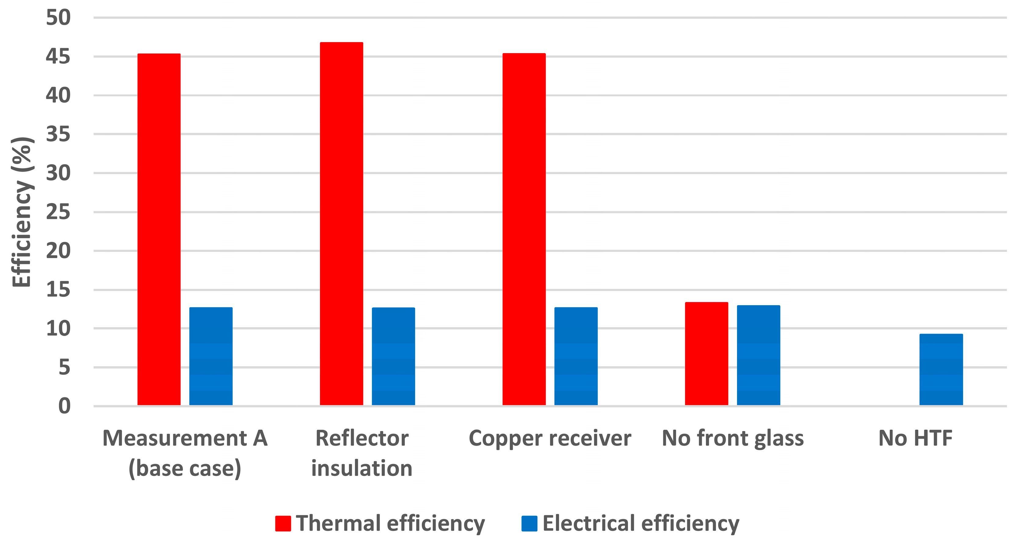
3.3.3. Collector Modification

Table 5. Performance of the different collector variations studied (T_amb = 18.6 °C, T_m = 35.1 °C).

	Back Side Cell Temperature (°C)	Top Side Cell Temperature (°C)	Thermal Power (w)	Electrical Power (w)
Measurement A (base case)	42.4	42.2	511	142.2
Reflector insulation	42.6	42.4	528	142.1
Copper receiver	42.3	42.1	512	142.3
No front glass	38.2	36.5	150	145.2
No HTF	105.7	105.2	0	103.6

presents three modifications, that have been suggested and studied, and later on compared with the base case presented in measurement A. To reduce the heat losses by convection in the collector box, insulation was applied on the backside of the reflector. This insulation increases the thermal power by 3% when working at a temperature of 23 °C above ambient (Figure 22).

To increase the heat transfer rate between the receiver and HTF, the receiver material was changed from aluminum to copper, due to the higher conductance of the copper. This change had no significant relevance in the collector output, which indicates that the aluminum is not the bottleneck for the transfer of heat between the solar cells and the HTF. It is important to point out that there is a very small temperature gradient across the 158 mm of the receiver width.

Another variation that has been studied was a collector without the front glass, in order to reduce the overall temperature inside the collector, since by removing the front glass, the hot air is released to the ambient. This effect also reduces the PV cells’ temperature and due to that, the electrical production increases by 2%. On the other hand, due to the lower temperature gradient, the thermal power decreased by 70% (T_amb = 18.6 °C, T_m = 35.1 °C). This result shows that, as expected, a glass cover is fundamental for any collector that has been expected to work at 10 °C above ambient temperatures.

4. Conclusions

The presented paper focused on the CFD modeling of a low concentrating PVT solar collector with an asymmetric reflector geometry produced by Solarus Sunpower. The presented CFD model was validated by the existing experimental data. The design of the collector, the installation of the set-up and the CFD model were described, analyzed and discussed. After the validation of results, the CFD model proved to be a powerful tool for solving the continuity, energy and momentum equations inside the collector, as well as helping to understand the collector´s behavior when variations to the design are introduced. Several variations were considered and compared with a base case of measurement A. Top side sensors 3 and 4 showed higher temperatures due to direct solar radiation. Top side sensor 2, located on the receiver core, showed nearly the same temperatures as the ones registered for the HTF. The back side sensor 1 (located far from the focal point) showed lower temperatures than the ones registered for the top side sensor 4.

As expected, the temperature of the HTF greatly affects the collector power, with both thermal and electrical efficiency decreasing with an increment in temperature. Under stagnation, the PV cells temperature reached a maximum of 105 °C (80 °C higher than standard temperature (25°C)) and the electrical production of the collector decreased by 32%. HTF, with an average temperature of 35.1 °C and 2.2 L/min flow rate, can decrease temperature to 42 °C. This 63 °C reduction in cell temperature caused a 25% increase in electrical efficiency. This result shows the importance of cooling.

With the aim of increasing the overall collector production, three modifications were studied. Firstly, by applying insolation on the back side of the reflector, the thermal power increased by 3%. Secondly, by changing the receiver material from aluminum to copper (due to the higher conductance), no relevant variations have been found, due to the low temperature gradient in the receiver.

Lastly, by removing the front glass, the electrical yield increased by 2%, which is caused by the lower temperature of PV cells. However, this also implies that the thermal yield is reduced by 70%, which means that this would not be a good trade-off from an energy output perspective. This result shows, as expected, that collectors for DHW require a front glass.

References

1. Masson-Delmotte, V.; Zhai, P.; Pörtner, H.-O.; Roberts, D.; Skea, J.; Shukla, P.R.; Pirani, A.; Moufouma-Okia, W.; Péan, C.; Pidcock, R.; et al. Global Warming of 1.5 °C. An IPCC Special Report on the Impacts of Global Warming of 1.5 °C; Intergovernmental Panel on Climate Change: Geneva, Switzerland, 2018. [Google Scholar]
2. Paris, 2015, Sustainable Innovation Forum. Available online: www.cop21paris.org (accessed on 17 November 2019).
3. Miller, O.D.; Yablonovitch, E.; Kurtz, S.R. Strong internal and external luminescence as solar cells approach the Shockley-Queisser limit. IEEE J. Photovolt. 2012, 2, 303–311. [Google Scholar] [CrossRef] [Green Version]
4. Kalogirou, S.A. Solar Energy Engineering: Processes and Systems, 2nd ed.; Elsevier: Amsterdam, The Netherlands, 2014. [Google Scholar]
5. Miljkovic, N.; Wang, E.N. Modeling and optimization of hybrid solar thermoelectric systems with thermosyphons. Sol. Energy 2011, 85, 2843–2855. [Google Scholar] [CrossRef] [Green Version]
6. Zondag, H.A. Flat-plate PV-Thermal collectors and systems: A review. Renew. Sustain. Energy Rev. 2008, 12, 891–959. [Google Scholar] [CrossRef] [Green Version]
7. Stylianou, S. Thermal Simulation of Low Concentration PV/Thermal System Using a Computational Fluid Dynamics Software. Master’s Thesis, Delft University of Technology, Delft, The Netherlands, 2016. [Google Scholar]
8. Chow, T.T. A review on photovoltaic/thermal hybrid solar technology. Appl. Energy 2010, 87, 365–379. [Google Scholar] [CrossRef]
9. Mbewe, D.J.; Card, H.C.; Card, D.C. A model of silicon solar cells for concentrator photovoltaic and photovoltaic/thermal system design. Sol. Energy 1985, 35, 247–258. [Google Scholar] [CrossRef]
10. Garg, H.P.; Adhikari, R.S. Conventional hybrid photovoltaic/thermal (PV/T) air heating collectors: Steady-state simulation. Renew. Energy 1997, 11, 363–385. [Google Scholar] [CrossRef]
11. Zondag, H.A.; De Vries, D.D.; Van Helden, W.G.J.; van Zolingen, R.C.; Van Steenhoven, A.A. The thermal and electrical yield of a PV-thermal collector. Sol. Energy 2002, 72, 113–128. [Google Scholar] [CrossRef] [Green Version]
12. Coventry, J.S. Performance of a concentrating photovoltaic/thermal solar collector. Sol. Energy 2005, 78, 211–222. [Google Scholar] [CrossRef]
13. Reichl, C.; Hengstberger, F.; Zauner, C. Heat transfer mechanisms in a compound parabolic concentrator: Comparison of computational fluid dynamics simulations to particle image velocimetry and local temperature measurements. Sol. Energy 2013, 97, 436–446. [Google Scholar] [CrossRef]
14. Buonomano, A.; Calise, F.; Vicidomini, M. Design, Simulation and Experimental Investigation of a Solar System Based on PV Panels and PVT Collectors. Energies 2016, 9, 497. [Google Scholar] [CrossRef]
15. Tyto, A. Performance Analysis of the Thermal Absorber of Solarus Photovoltaic-Thermal Collector. Master’s Thesis, Eindhoven University of Technology, Eindhoven, The Netherlands, 2017. [Google Scholar]
16. Li, W.; Paul, M.C.; Sellami, N.; Mallick, T.K.; Knox, A.R. Natural convective heat transfer in a walled CCPC with PV cell. Case Stud. Therm. Eng. 2017, 10, 499–516. [Google Scholar] [CrossRef]
17. Yi, S.P. Advanced Integrated Numerical Model for a Concentrated Photovoltaic-Thermal (CPVT) Collector. Master’s Thesis, Eindhoven University of Technology, Eindhoven, The Netherlands, 2018. [Google Scholar]
18. Campos, C.S.; Torres, J.P.N.; Fernandes, J.F.P. Effects of the Heat Transfer Fluid Selection on the Efficiency of a Hybrid Concentrated Photovoltaic and Thermal Collector. Energies 2019, 12, 1814. [Google Scholar] [CrossRef] [Green Version]
19. Tiemessen, M. Thermal Modelling and Experimenting on Solarus’ PowerCollector. Master’s Thesis, Eindhoven University of Technology, Eindhoven, The Netherlands, 2019. [Google Scholar]
20. Gomes, J. Assessment of the Impact of Stagnation Temperatures in Receiver Prototypes of C-PVT Collectors. Energies 2019, 12, 2967. [Google Scholar] [CrossRef] [Green Version]
21. Solarus Sunpower Sweden. Available online: www.solarus.se (accessed on 17 November 2019).
22. Adsten, M.; Helgesson, A.; Karlsson, B. Evaluation of CPC-collector designs for stand-alone, roof-or wall installation. Sol. Energy 2005, 79, 638–647. [Google Scholar] [CrossRef]
23. Rönnelid, M.; Perers, B.; Karlsson, B. Construction and testing of a large-area CPC-collector and comparison with a flat plate collector. Sol. Energy 1996, 57, 177–184. [Google Scholar] [CrossRef]
24. Bernardo, R.; Davidsson, H.; Gentile, N.; Gomes, J.; Gruffman, C.; Chea, L.; Mumba, C.; Karlsson, B. Measurements of the electrical incidence angle modifiers of an asymmetrical photovoltaic/thermal compound parabolic concentrating-collector. Engineering 2013, 5, 37. [Google Scholar]
25. Bergman, T.L.; Incropera, F.P.; DeWitt, D.P.; Lavine, A.S. Fundamentals of Heat and Mass Transfer, 7th ed.; John Wiley & Sons: Hoboken, NJ, USA, 2011. [Google Scholar]
26. Fluent, A.N.S.Y.S. User’s Guide Release 16.2; Ansys Inc.: Pittsburgh, PA, USA, 2015. [Google Scholar]
27. Guarracino, I. Hybrid Photovoltaic and Solar Thermal (PVT) Systems for Solar Combined Heat and Power. Ph.D. Thesis, Imperial College London, London, UK, 2017. [Google Scholar]
28. Howell, J.R.; Menguc, M.P.; Siegel, R. Thermal Radiation Heat Transfer, 4th ed.; Taylor & Francis: Milton Park, UK, 2002. [Google Scholar]
29. García-Gil, Á.; Casado, C.; Pablos, C.; Marugán, J. Novel procedure for the numerical simulation of solar water disinfection processes in flow reactors. Chem. Eng. J. 2019, 376, 120194. [Google Scholar] [CrossRef]
Figure 1. Solarus Power Collector.
Energies 13 01669 g001
Figure 2. Top view of the concentrated photovoltaic-thermal collector (CPVT) collector. The water connections are marked in blue and the electrical connections in red [20].
Energies 13 01669 g002
Figure 3. The detail of geometric concentration (all dominations in mm).
Energies 13 01669 g003
Figure 4. Concertation of solar radiation on the receiver and location of the focal point.
Energies 13 01669 g004
Figure 5. The geometry of the collector and details of the receiver.
Energies 13 01669 g005
Figure 6. Mesh of the collector.
Energies 13 01669 g006
Figure 7. (a) Solar Collector Test Rig at Gävle University. (b) The tested Solarus CPVT collector.
Energies 13 01669 g007
Figure 8. Schematic of the experimental setup.
Energies 13 01669 g008
Figure 9. The placement of each temperature sensor on the different layers of the receiver.
Energies 13 01669 g009
Figure 10. Measurement A: layers, water and ambient temperatures and solar radiation. The flow rate of measurement: 2.2 L/min.
Energies 13 01669 g010
Figure 11. Measurement B: layers, water and ambient temperatures and solar radiation. The flow rate of measurement: 1 L/min.
Energies 13 01669 g011
Figure 12. Measurement C: layers, water and ambient temperatures and solar radiation. The flow rate of measurement: 2.2 L/min.
Energies 13 01669 g012
Figure 13. Simulated temperature distribution over the cells on both sides of the receiver (outer part) for measurement A.
Energies 13 01669 g013
Figure 14. Measurement A: experimental results versus Computational Fluid Dynamics (CFD) results.
Energies 13 01669 g014
Figure 15. Measurement B: experimental results versus CFD results.
Energies 13 01669 g015
Figure 16. Measurement C: experimental results versus CFD results.
Energies 13 01669 g016
Figure 17. Discrete Ordinates (DO) radiation contour inside the collector.
Energies 13 01669 g017
Figure 18. Temperature contours inside the collector.
Energies 13 01669 g018
Figure 19. Velocity streamlines inside the collector.
Energies 13 01669 g019
Figure 20. Thermal and electrical power of the collector for different tilt angles.
Energies 13 01669 g020
Figure 21. Thermal and electrical efficiency of the collector for different HTF temperatures.
Energies 13 01669 g021
Figure 22. The thermal and electrical efficiency for collector’s modifications.
Energies 13 01669 g022