Abstract
The dynamic bottom-up modelling of greenhouse gas (GHG) abatement measures in industry makes it possible to derive consistent transformation paths on the basis of heterogeneous, process-specific developments. The main focus is on the development of a transparent methodology for small-scale modelling and combination of individual GHG abatement measures. In this way, interactions between GHG abatement measures are taken into account when deriving industrial transformation paths. The presented three-part methodological approach comprises the preparation (1) and implementation (2) of GHG abatement measures as well as the resulting effects on the output parameters (3) in a technology mix module. In order to consider interactions in the measures implementation, year-specific overall measure matrices are created and prioritised based on the GHG abatement costs. Finally, the three-part methodology is tested in a consistent technology mix scenario. The results show that the methodology enables integrated industrial technology mix scenarios with a high level of climate ambition based on a plausible development of energy consumption and emissions. Compared to the reference scenario, the process-and energy-related emissions decrease by 90 million tCO2 (77% of the 1990 level in 2050). The developed methodology and the related technology mix scenario within the framework of the bottom-up industry model SmInd can support strategic decision-making in politics and an efficient transition to a greenhouse gas neutral industry.
1. Introduction
While considerable attention is paid to defossilising the supply, transport and household sectors, knowledge of how greenhouse gases can be abated in industry sector is lagging behind [1,2,3]. An analysis of recent German energy and climate scenarios shows that a combination of different GHG abatement measures in the industrial energy transition is usually more effective in achieving the climate goals [4,5,6,7], than focusing on stringent transformation paths without an openness to different technologies [8]. However, industrial heterogeneity leads to a wide range of GHG abatement technologies [9,10,11,12], some of which often show interdependencies [1]. Therefore, the combination of GHG abatement measures by modelling a consistent industrial technology mix scenario often leads to difficulties. For example, the order of GHG abatement measures in the implementation process is crucial for the development of efficient transformation paths. The implementation order in currently existing scenarios is often estimated exogenously by experts [4,13]. A few industrial models make it possible to compute technology-independent, consistent transformation paths that take interdependencies between individual small-scale GHG abatement measures into account [14]. With the many and complex ways in which GHG abatement measures affect industrial production volumes, energy consumption and emissions [15], as well as the related interdependencies between the individual measures, further problems arise in modelling industrial scenarios. Existing German industrial models have so far addressed these problems only to a limited extent. Therefore, the following section provides an overview of the current research state of numerous German industrial models and outlines further research needs. The analysis serves as a basis for this research contribution and further objectives.
The FORECAST Industry simulation model of the Fraunhofer Institute for Systems and Innovation Research (ISI) maps German and European industry from the bottom-up using five submodules. The submodules comprise energy-intensive processes, furnaces, electric motors and lighting, steam and hot water as well as space heating and cooling [14,16]. Energy-and emission-intensive processes are modelled using activity parameters such as production volume and specific consumption [17]. To reflect the development of less energy-intensive processes, generic parameters such as gross value added are used [14,17]. Similarly the development of activity parameters, as well as the framework parameters based on forecast data are specified exogenously in the model. GHG abatement options for energy efficiency, fuel switch, CO2-capture and storage as well as recycling management and material efficiency are implemented in the model [14] from a microeconomic perspective [16]. The methodology for implementing GHG abatement measures depends on the respective submodule [14]. The use of technology in the submodule “Steam and Hot Water”, for example, is determined by a utility function which, in addition to the classic CAPEX and OPEX, also includes technology revenues and state subsidies [18]. In addition, the technology stock is recorded in order to make the investment decision based on economic developments and natural reinvestment cycles. Also, the fuel switch is carried out by application of a utility function [19]. Investments in efficiency technologies are made taking the related amortisation-time into account [14]. The measures are prioritised with regard to the resulting present value of the technology investment. The transformation speed is therefore model-endogenous and partly non-linear [14]. Diffusion curves are implemented for several submodules to specify the transformation speed [14]. The diffusion of energy efficiency measures in the assets is based, for example, on logistic growth curves depending on the amortisation period. Simulation results are energy carrier, application and technology-specific energy consumption, load profiles, emissions and technology costs [14,17]. Analogously to process heat, process cooling is also subdivided by temperature level [17,20]. At industry level, a distinction is made between seven economic branches and applications as well as 15 energy carriers. FORECAST Industry is used in energy and climate studies [21,22].
In order to calculate the future economic branch-specific final energy consumption by energy carrier and application, the Prognos model maps industry in a bottom-up manner using activity parameters [5,23,24,25]. Based on the German energy balance and industry statistics, the model distinguishes between up to 14 economic branches, 26 applications and 35 energy carriers [5,24]. In order to determine future energy consumption, the branch-specific value density (Wh/€) and the specific energy consumption (Wh/kg) for particularly energy and emission-intensive branches are decisive variables [5]. In addition to energy-and emission-intensive industries, cross-sectional technologies are treated separately at industry level [24]. Economic branch-specific developments in gross value added (€) and production volume provide the basis for calculating the future final energy consumption of the respective branch [5,23]. Prognos uses the VIEW economic model to extrapolate the economic branch-specific gross value added and the number of employed persons [26]. Efficiency improvements, energy carrier substitutions and value density developments observed in the past are transferred to the future on a trend basis [24]. Measure clusters address technical changes in industrial production processes and are translated into economic cash flows [23]. The branch-specific GHG abatement measures are prioritised according to macroeconomic abatement costs. In addition to GHG abatement costs, practical restrictions as well as social acceptance are taken into account [5]. Furthermore, the saving potentials and costs of the GHG abatement measures are dynamically forecasted [23,25]. The diffusion of efficiency measures is based on replacement rates which are oriented on the lifetime and profitability of the facility replacement [24]. In addition, a certain technology modification is included in the more efficient facilities [24]. The simulations result in industry-specific energy consumption, energy costs and emissions [25]. The Prognos industrial model is used, inter alia, to calculate energy and climate-policy scenarios in [5,25].
The industrial module of the “Price-Induced Market Equilibrium System” (Primes) model of the University of Athens calculates the energy and emission development of the 28 EU member states [23,27,28]. Industry is divided into nine main and 24 sub-branches. In turn, the branches include individual processes and cross-sectional technologies [27]. The energy demand of the processes, cross-sectional technologies and branches is derived from the General Equilibrium Economic Model [27]. The Primes Industrial Model contains, inter alia, GHG abatement measures for process route, energy carrier, raw material switch and CO2-capture [14]. The implementation of the GHG abatement measures is determined from a microeconomic perspective in a cost-minimising, non-linear optimisation. The implementation of the GHG abatement measures is performed according to the economic optimality, the technology lifetime, the available capacity, the market penetration depending on the relative costs and risk, and the technology readiness level. Branch-and country-specific energy consumption and emissions form the model output [28].
The industrial module of the WISEE model is a bottom-up model of the Wuppertal Institute that maps production technologies of selected value chains using resources, product and energy flows [13]. Industrial simulations are based on at least twelve industrial processes. Parameters gathered in stakeholder processes provide the basis for deriving exogenous industrial transformation paths with the model. The focus lies on manufacturing processes, by means of which energy efficiency and GHG abatement potentials are highlighted. To deduce system-optimal, endogenous transformation paths for future industrial development is not part of the model [13]. Energy consumption is determined bottom-up via specific energy consumption and production volumes. Future emissions are calculated by multiplying energy consumption and emission factors. The model is based on three GHG abatement options: more energy-efficient production, increased material and resource efficiency and intensified recycling [13]. There is no model-endogenous rather a model-exogenous implementation of the three GHG abatement options [13]. The model results include emissions and final energy consumption subdivided by production and manufacturing processes [29].
In the industrial model of the Institute of Energy Economics at the University of Cologne (ewi) (DIMENSION+), in contrast to the Prognos and ISI models, no industry-related endogenous bottom-up modelling is carried out. Economic branch-specific transformation paths are determined top-down from a macroeconomic perspective [4,23,30]. The economic branch-specific development of the final energy consumption is determined on the basis of existing GHG abatement clusters, not on the endogenous implementation of individual GHG abatement measures [23]. Annual developments in gross value added, efficiency increases and recycling rates in industry serve as a database [30,31]. Historical developments and expert interviews provide the background. Capital costs are not taken into account in the industrial model when determining exogenous transformation paths [4,30,31]. Energy consumption and emissions at industry level as well as from individual energy-and emission-intensive processes are provided with model calculations.
The literature review supports the assumption that very few industrial models provide technology-independent, consistent transformation paths for German industry. For example, in the DIMENSION+ and WISEE models there is no endogenous implementation of individual measures, rather industrial transformation paths are predominantly exogenously defined [13,30]. With FORECAST Industry [14], the Prognos Industry Model [24] and the Industry Module of the Primes Model [27], it is possible to map transformation paths for German industry in consistent technology mix scenarios. However, “Primes Industry” is strongly focused on European industry [28]. The exact calculation and implementation methodology of Prognos AG’s industrial model for the combination of various GHG abatement measures and the consideration of interactions between individual measures remains unclear [24], as these are not fully accessible to the public. In addition, [24,27] do not describe the level of detail with which GHG abatement options are implemented in the model. However, [24] proposes the conclusion that GHG abatement measures in the Prognos industrial model are only implemented at branch-and not process-level. FORECAST Industry takes a microeconomic perspective, systemic connotations are not the main emphasis of the simulations. Heterogeneous industry also requires differentiated approaches in order to be able to use different perspectives in the derivation of industrial transformation paths.
Based on the research needs outlined above, the main objective of this publication is to develop a transparent methodology for small-scale modelling of individual GHG abatement measures in German industry and to test them on the basis of selected model calculations in a consistent technology mix scenario. This includes the development of an integrated open-independent modelling method that allows the combination of GHG abatement measures in a technology mix module at individual measure level and takes interactions of measure implementation into account. Restrictions and measure implementation, as well as methodological characteristics of scenario development with a time horizon up to 2050 are described in detail. In addition to the developed methodological, exemplary paths for energy consumption, emissions and other relevant industrial parameters up to 2050 are presented. The technology mix scenario assumes a high level of industrial climate ambition. Another objective is illustrating the effects of learning curves on technology development in the industry sector by means of sensitive model calculations.
2. Materials and Methods
The sector model industry (SmInd) conducts energy and emission dynamic calculations with a time horizon up to 2050 [1,32]. SmInd has several substructures that divide the whole of German industry, in a top-down manner, into 14 branches [33]. In the energy carrier application matrix (EAM), the consumption of economic branches is combined by energy carrier and application. A distinction is made between ten electricity (space heating, hot water, process heat, process cooling, air-conditioning, compressed air, pumps, information and communication technology, other mechanical energy, lighting) and three fuel (process heat, mechanical energy, space heating and hot water) applications. For “process heat” at branch level, a subdivision by temperature is provided as well [33,34], which is based on [35]. A distinction is made between four temperature levels (Process heat less than 100 °C, between 100 °C and 500 °C, between 500 °C and 1000 °C and above 1000 °C). In order to perform bottom-up analyses, 22 selected energy-and emission-intensive processes are assigned to the economic branches [1,32].
2.1. Description of the Basic Functionality of the Model
Figure 1 summarises the bottom-up technology modelling in SmInd. Individual production facilities are assigned to processes that are mapped using activity parameters. For these processes, annual production volumes [22,25], specific electricity and fuel consumption are available [1]. In turn, the processes are subordinated to economic branches on the left side of the figure. As part of the modelling of the technology mix scenario in SmInd, the processes are extended by a fuel distribution [36,37,38,39,40,41]. Cross-sectional technologies are modelled at a non-process-specific industrial level based on [42]. The model distinguishes ten cross-sectional technologies. Some examples are shown in Figure 1 on the right side. In the middle of Figure 1 the different hierarchical levels in the model are shown. A total of four hierarchy levels are distinguished in the model.
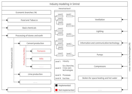
Figure 1.
Industrial technology modelling in SmInd. Terms written in black are already implemented in the model. The red terms are not yet available in the model, but should be implemented in the future.
The functional principle of SmInd and its integration into the FfE model landscape (right-hand side) is shown in Figure 2. The figure also contains the level of detail of individual input and output variables on the left side. The operation base is the reference scenario, which contains the energy and emission-oriented reference development of German industry from 2015 to2050. In the reference scenario, the branch-specific energy consumption by energy carrier is determined based on existing scenarios up to the target year. In turn, this data serves as a basis for specifying energy consumption by application and temperature level according to [33,35]. Based on the energy carrier precise consumption, emission factors are used to compute the energy-related emissions of the reference scenario. Specific process emission factors are also used to determine the process-related emissions based on the production volume of the process. In addition to the bottom-up calculation, process-related emissions are also distributed top-down to the economic branches on the basis of the national inventory report [1]. The energy costs are based on the given energy prices and energy consumption data and are stored depending on the specific energy carrier. The reference scenario and the activity parameters are the baseline of all other implemented and calculated scenarios [1,32].
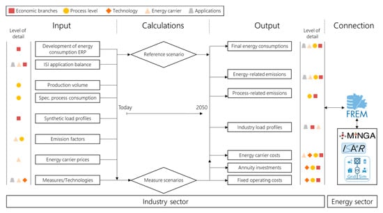
Figure 2.
Inputs and outputs of SmInd and integration into the FfE model landscape.
In the following section, the methodical and implementation-oriented enhancement of SmInd based on a technology mix module is developed by combining all available GHG abatement measures of the model and considering interdependencies between them. The SmInd modelling process is conducted using Matlab.
2.2. Overview of the Methodological Procedure
The procedure consists of four main steps, as shown in Figure 3.
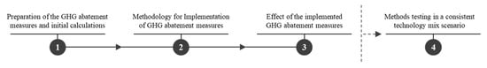
Figure 3.
Overview of the methodological procedure.
In step (1), the individual, small-scale GHG abatement measures and the associated parameters are prepared and converted into a matrix containing all relevant data. In addition, measures for generic efficiency progress are derived from existing ones for the portion of energy consumption that is not covered by individual GHG abatement measures. In step (2), a methodology for implementing and combining small-scale GHG abatement measures in the industry sector is developed. In this context, a new methodology of measure prioritisation as well as implementation-related restrictions are presented. In addition, learning curves are taken into account. In the third step (3), a modelling approach is developed, analysing the effects of GHG abatement measures on energy consumption, emissions and production volumes. Interdependencies between the individual GHG abatement measures are taken into consideration as well. In addition, changed CAPEX and OPEX are calculated, which have accrued for the individual abatement measures and for the whole industrial transformation path. In the fourth step (4), the methodology is tested in a consistent technology mix scenario.
2.3. Preparation of GHG Abatement Measures and Initial Calculations
The technology mix module combines both process-specific and process-unspecific GHG abatement measures. Process-unspecific GHG abatement measures are termed as cross-sectional measures. Cross-sectional measures refer to applications such as industrial lighting or gas consumption in the entire industry sector, whereas process-specific GHG abatement measures are always assigned to a specific process such as steel production. Figure 4 summarises the allocation of the technology mapping to the measure categories in the technology mix module.
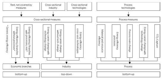
Figure 4.
Assignment of modelled technologies to the measure categories and effect level.
Process measures are divided into five measure categories in the technology mix module and affect the production processes as well as the associated industrial production facilities (Furnaces, electrolysers, mills and other industrial production facilities). Efficiency measures reduce the energy consumption of the processes. The process route change describes the conversion of conventional to new production processes for manufacturing the same product. In the technology mix module, it is possible to switch from one reference to several substitution processes. The energy carrier change with technology change at process level describes the conversion of existing facilities enabling the switch to climate-neutral energy sources. CO2-capture reduces both energy and process-related emissions in selected industrial production processes. No CO2-storage takes place because the captured CO2 is used in the supply sector to produce synthetic methane. The material and resource efficiency is indirectly considered in the model via the development of the production volumes and the specific process consumption and is therefore not described in more detail in the following sections. Process measures are always linked to the activity parameters of the production process. A detailed description of the measure categories can be found in [1,32]. The description of the technology mix scenario provides examples in the Section 1.
The technology mix module also distinguishes between five cross-sectional measure categories. Increasingly efficient cross-sectional technologies (lighting, electric drives, boilers for space heating and hot water generation and other cross-sectional technologies) reduce energy consumption compared to the reference scenario. The use of industrial heat pumps and electrode heating boilers as a result of the energy carrier change with technology change at cross-sectional level also enables the electrification of fuel applications in low-temperature heat. In addition, energy carrier changes are implemented without technology change, substituting natural with synthetic gas or coal with biomass. If coal is still used in industrial processes at the end of the scenario path, it can be ex-post replaced with a climate-neutral solid fuel over a period of five years.
The efficiency measures at process and cross-sectional level cover a large part of industrial energy consumption. To model a consistent technology mix scenario, both the remaining consumption of the economic branches with processes and economic branches without process efficiency must be assigned with generic efficiency progress. For economic branches that contain energy-and emission-intensive processes with relevant efficiency measures, the necessary parameters for the formation of a generic economic branch-specific measure are computed on the basis of the existing process measures. For this purpose, the mean of the relevant parameters is calculated. Average electricity and fuel savings as well as the associated CAPEX and OPEX form the basis of the generic efficiency measure. Since no relation to the production volume of energy-intensive processes or the number of factories (cross-sectional technologies) is possible, the diffusion of efficiency improvements also depends on the average of implemented efficiency measures. Therefore, generic efficiency measures differ from the specific parameters of the process and other cross-sectional measures. Therefore, the absolute change in electricity and fuel consumption is inserted in the measure matrix (kWh) [1]. CAPEX and OPEX (€/kWh) are incurred for each kilowatt hour by implementation of generic efficiency at industry level. The described methodology of generic energy efficiency applies analogously to economic branches without processes. However, in this case, average values of all relevant process efficiency measure parameters are formed in order to generate generic, economic branch-specific energy efficiency measures. The calculated generic efficiency per economic branch is divided by the average lifetime of the relevant process efficiency measures. Thus, annual parameters of the generic energy efficiency measures are generated. The generic efficiency measures at economic branch level are considered as ordinary efficiency measures in the measure matrix.
To model individual GHG abatement measures in industry and to combine them in a technology mix module, the existing model structure has to be changed from the implementation of measure clusters to individual GHG abatement measures [1]. The resulting overall matrix contains 27 parameters per GHG abatement measure that are required for the measure implementation and combination (see Appendix A, Table A1). The technology mix module combines 117 individual measures for GHG abatement, which can be assigned to ten measure categories (see Figure 5). Accordingly, up to nine different implementation and evaluation logics are required in the technology mix module depending on the measure category.
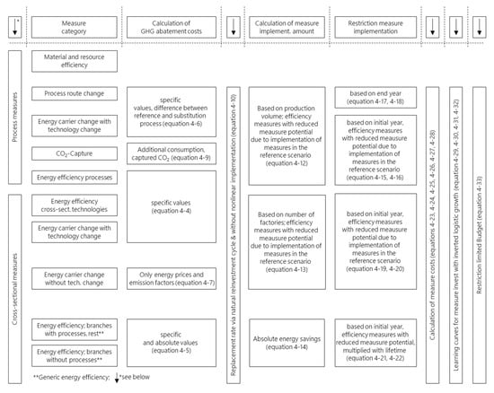
Figure 5.
Assignment of equations according to measure categories to implement GHG abatement measures in TMI.
To determine the effect of individual GHG abatement measures or measure categories, filter mechanisms are available in the technology mix module allowing selection of individual measures or categories. Thus, it is possible to compute and analyse the effects of individual GHG abatement measures or categories on energy consumption, emissions and process costs, economic branches or industry as a whole. As a result of the initial calculations, year-specific matrices with small-scale GHG abatement measures filtered according to predefined criteria are available. These are used as a basis for the temporally bound implementation of measures in the technology mix module.
2.4. Methodology for Implementing GHG Abatement Measures
At the beginning of the measure implementation, an individual measure matrix is available in the technology mix module for each year, which contains all year-specific relevant GHG abatement measures. In the technology mix module, it is possible to implement the measures with fundamentally different implementation logic. Two implementation logics are already implemented in the model:
- Implementation of the GHG abatement measures as a result of a ranking specified by expert assessment
- Implementation of measures according to annual, static GHG abatement costs
A target commitment is possible for the implementation logic, whereby the level of climate ambition in industry can be specified (e.g., specified GHG abatement by 2030). In the following technology mix module, the measures are implemented according to annual, static GHG abatement costs.
Figure 5 shows the basic methodology for the GHG abatement measure implementation depending on the measure category. The allocation of the equation to the respective implementation step and the measure category can also be taken from Figure 5.
As a result of the annual change in hourly emission factors and energy prices, each individual measure causes year-specific GHG abatement costs. If, in addition, learning curves, which influence the investment costs of GHG abatement measures depending on the implementation degree, are used, the basis for calculating year-specific GHG abatement costs changes. To compute the year-specific, static GHG abatement costs for each measure, the mean of the fluctuating electricity and fuel prices over the year is determined according to [43]. To compute GHG abatement costs, the annuity factor has to be calculated, which is defined according to [44].
The calculation of the GHG abatement costs is based on Equation (1) [45]. According to [45] this equation is only permissible if a measure leads to a CO2 abatement compared to the reference technology. A positive denominator of the equation is therefore a basic prerequisite for its validity:
| €/tCO2) abatement costs of measure j | (tCO2) emissions with measure |
| (€) costs of reference | (tCO2) emissions reference |
| (€) costs of measure | (tCO2) change in emissions |
| (€) change in costs | |
The calculation of the year-specific, static GHG abatement costs per measure in the model depends on the respective measure category. Dependent on the measure category, various parameters must be included. The full costs as given in Equation (1) are not used to calculate the GHG abatement costs, but only the changed costs resulting from the implementation of the GHG abatement measure.
The GHG abatement costs of the measure category “Energy efficiency processes” are calculated in the technology mix module according to Equation (2). The formula contains specific parameters related to the production volume:
| (€) abatement costs efficiency process of measure j | (€/MWh) price for electricity |
| () investment costs | (€/MWh) price for fuel f |
| (1/a) annuity factor | (%) quota of fuel f in the process |
| () fixed operation costs | (tCO2/MWh) emission factor electricity |
| () change in electricity | (tCO2/MWh) emission factor of fuel f |
| () change of fuel f | (dL) measure j |
| (dL) number of fuels | ∅ (dL) symbol for average of a variable |
The differential costs consist of the additional annuity investment and fixed operating costs as well as the changed energy costs due to the measure in the numerator. The denominator includes the changed emissions compared to the reference case. The changed energy consumption is multiplied by the average energy carrier-specific emission factors in the denominator. As fuel-specific consumption changes are not available in the measure matrix, the annual fuel distribution of the process is used to calculate the GHG abatement costs. Equation (3) is used by analogy for the cross-sectional measure of the measure category “Energy efficiency—cross-sectional technologies” at industry level. Instead of the fuel distribution at process level, the distributions at industry level are used. In addition, the specific values do not refer to tonnage, but to the number of factories where the measure can be applied. This also applies to the cross-sectional measure of the measure category “Change of energy carrier with technology change” (see Equation (3)).
Equation (3) is used to calculate GHG abatement costs for generic efficiency. For this measure category, the energy change is stored in the overall measure matrix without a specific reference value. Accordingly, the calculation is performed on the basis of absolute values. To calculate the energy consumption for each energy carrier, the change in fuel consumption is used on the basis of the annual fuel distribution at industry level:
| (€) abatement costs efficiency branch of measure j | (MWh) change of electricity |
| (€/MWh) investment costs | (MWh) change of fuel f |
| fixed operation costs | (%) quota of fuel f in branch |
A different methodology for calculating GHG abatement costs is used for the process route change, because the production volume of the process routes changes as a result of the measure. As different routes also have different fuel distributions, the energy carrier distribution changes as a result of the measure. This results in different absolute fuel costs and emissions. By switching from blast furnace to H2-steel, for example, hydrogen is mainly used as a reductant instead of coke, which entails different energy carrier costs.
To calculate the GHG abatement costs of the process route change, the change in the fuel-specific energy costs between the reference and substitution process of the individual process routes is equal to the product of specific consumption, the share of the fuel in the total fuel consumption and the average fuel price in the numerator. In the denominator, the change in emissions resulting from the changed fuel allocation is equal to the difference between the emissions from the reference and substitution processes. In turn, the emissions are equal to the product of the specific consumption, the share of the respective fuel in the total fuel consumption and the average emission factor. In addition, the changed process-related emissions are taken into account (see Equation (4)):
| (€) abatement costs, production route change | (dL) reference process |
| (MWh/) specific consumption | (dL) substitution process |
| () process emission factor | |
In addition to the process route change, the equation can be used to compute GHG abatement costs for the measure category “Change of energy carrier with technology change” at process level (see Equation (5)). A target distribution of the fuels must be defined for the energy carrier change with technology change, because the fuel distribution is not fixed in case of a process route change.
The GHG abatement costs for the cross-sectional measure category “energy carrier change without technology change” are calculated according to Equation (5). Changes in energy consumption, investments and fixed operating costs are not expected as there is no change in technology. Therefore, the abatement costs result from the difference in energy prices or emission factors between substitution and reference energy carriers in the numerator or denominator:
| (€) abatement costs energy carrier change without technology change | (dL) substitution |
| (dL) reference | |
| (dL) energy carrier | (dL) number of energy carriers |
The GHG abatement costs of CO2-capture take into account both the changed energy-related and process-related emissions. Initially, the existing direct energy-related emissions per tonne of production volume of the process without CO2-capture are determined (see Equation (6)). The GHG abatement is calculated from the difference between saved and additional emissions as a result of CO2-capture. In turn, the captured emissions consist of process-related, existing energy-related and direct energy-related emissions resulting from the increase in energy consumption. When calculating the abated emissions, the capture rate, which varies per process, must be taken into account (see Equation (7)). The additional emissions are subtracted from the abated emissions resulting from the use of CO2-capture. These consist of the additional indirect emissions and the additional direct emissions that cannot be captured:
| (€) abatement costs | (%) rate of CO2-capture |
| () production volume | () direct emissions of the process |
Next, the complete matrix of measures is prioritised according to the calculated GHG abatement costs. Accordingly, measures with lower GHG abatement costs are preferably implemented. The prioritised measure matrix is determined and processed on an annual basis. The year-specific implementation of each individual GHG abatement measure in SmInd depends on the following two fundamental restrictions:
- Full implementation of the measure
- Budget restriction
To comply with the first restriction, criteria must be observed that describe the complete implementation of a GHG abatement measure. An individual, annual measure implementation amount is calculated for each individual measure. Irrespective of the measure category, the calculation of the implementation amount is based on the annual replacement rate [32]. Each GHG abatement measure is assigned to a lifetime, which is used to determine the replacement rate of the technologies according to Equation (8):
| (%/a) replacement rate per year of measure j | (a) lifetime of measure j, const |
As a first step, it is assumed that the technologies are renewed at the end of their lifetime. The natural replacement rate per year describes the natural reinvestment cycles over the lifetime of an technology. The measure category “energy carrier change without technology change” does not consider a technology lifetime. On the basis of internal expert estimates based on developments in the supply sector, it is determined at what transformation rate the energy carrier change can be conducted without technology change.
As a second step, it is also possible to apply a non-linear measure ramp-up in the technology mix module. The following function could be used for a nonlinear measure ramp-up (see Equation (9)):
| (%/a) replacement rate per year of measure j | (a) lifetime of measure j, const |
| (a) time | |
In the following calculations and evaluations, a linear measure ramp-up with natural replacement rates is assumed for each individual measure.
The application factor is also required for calculating the implementation amount [32]. Application factors reflect limitations with regard to market penetration and the associated existing technologies of industrial production processes [46]. The application factors of the GHG abatement measures are taken from the literature or are estimated by industry experts [46].
The calculation methodology of an implementation amount varies dependent on the measure category. To calculate the implementation amount for process measures according to Equation (10), the production volume of the process is used [32]:
| () measure implementation amount according to production volume per year | () production volume, initial year |
| (%) application factor | () production volume, year t |
| (%/a) replacement rate per year | (%) reduced measure potential |
The equation is divided into two parts: In the first part, the implementation amount is calculated using the start production volume (part 1). Due to the already partially existing implementation amount in the reference scenario, the potential for measures in the technology mix module must be reduced. This only applies to energy efficiency measures. The first part of the equation only changes depending on the natural replacement rate per year. In the second part (part 2), the annually fluctuating production volumes are taken into account. For this purpose, the difference between the production volume of the current year and the previous year is calculated and multiplied by the replacement rate per year. The production volumes of the processes in the simulation model are exogenously defined for the period between 2015 and 2050 [22,25]. A distinction is made between three production volume fluctuation cases:
Case 1—The production volume increases compared to the previous year: If the production volume increases in time step t compared to the previous year (t − 1), the implementation amount for the time step t increases as well. The additional production volume of the industrial process is however, not fully added to the converted production volume, but multiplied by the replacement rate. In this context, it should be noted that the additional production volume is also produced with older facilities that were not previously fully utilised. An industrial production volume increase, would first and foremost contribute to the use of existing facility production capacities. The construction of a new facility to accommodate an additional production volume can only be assumed above a certain threshold value. Consequently, the additional production volume is subject to a replacement process in a realistic manner.
Case 2—The production volume decreases compared to the previous year: If the production volume in time step t decreases compared to the previous year (t − 1), the implementation amount also decreases in year t. However, the decreasing production volume of the industrial process is also not fully subtracted from the implemented production volume. It is taken into account that not only does the production volume of the production processes equipped with the enhanced technology decrease, but also that of all existing facilities.
Case 3—The production volume remains constant compared to the previous year: As the production volume does not change compared to the previous year, the implementation amount for the current year is only influenced by the change in the replacement rate. The replacement rate in the technology mix module is constant as long as natural replacement rates based on lifetimes are used.
Cross-sectional measures are implemented according to Equation (11). Cross-sectional measures refer to overall industrial parameters. Therefore, their implementation is not linked to the production volume of a process, but based on the number of factories for which the GHG abatement measure can be applied:
| () measure implementation amount according to number of factories per year | (dL) number of factories, year t |
| (dL) number of factories, initial year | |
For the reason that only efficiency measures are implemented in the reference scenario, there is no limitation of the measure potential for all other measure categories. In this case, the reduced measure potential is equal to 1. For generic energy efficiency, the measure implementation is linked to the average lifetime of other efficiency measures. Accordingly, the replacement rate is already allowed for by the annual embedding of the measure in the measure matrix itself. Moreover, no effect-reducing application factor is considered. Correspondingly, the annual measure implementation amount results from the energy savings, implemented as shown in Equation (12):
| () measure implementation amount according to energy savings per year |
The criteria for the full implementation of a measure also differ with regard to the measure category. Process measures are considered fully implemented as soon as the entire production volume is produced with or supported by the technology (see Equations (13) and (14)):
| (| f | MWh) measured potential of j |
When a process route is changed, the following equation is used for complete implementation due to the natural production fluctuations (see Equations (15) and (16)). The fluctuating production volume after the complete implementation of the process route change measure is distributed evenly over the remaining process routes via a production volume module:
| () measure implementation amount process route change |
The complete implementation of the cross-sectional measures is based on the annual number of factories for which the measure is implemented. The initial measure potential is calculated on the basis of Equation (17). The complete implementation of cross-sectional measures is therefore completed if Equation (18) applies:
The full implementation of generic energy efficiency measures is determined by Equations (19) and (20). The measure potential is included in the reference scenario on the basis of the already implemented measures, the lifetime and the limited measure potential due to the already increased efficiency:
If a GHG abatement measure is fully implemented, it is removed from the subsequent measure matrices on an annual basis. In addition to the implementation, the equations also serve for the “explementation”, i.e., the removing of measures. A fictitious, negative production volume or number of factories is used to remove measures, which is subtracted from the implementation amount. Especially in scenarios with a time horizon up to 2050, the explementation is a relevant instrument for addressing technologies that bridge the gap to climate-friendly energy technologies.
In addition to the complete implementation of a measure, the budget restriction must also be adhered. In SmInd, the budget restriction describes the year-specific budget for the industry sector, which limits the annual measures implementation. Initially, the costs arising from the GHG abatement measures have to be computed. The measure costs are divided into investments and fixed operating costs. The variable operating costs, which are mainly caused by changes in energy consumption and energy prices, are not taken into account in the budget approach.
To calculate the total annuity investment, the annuity must first be determined according to Equation (21). Afterwards, a matrix is constructed in which the annuity investments over the lifetime are entered line by line (see Equation (22)). To determine the annual annuity investments, the matrix is summed column by column (see Equation (23)):
| (€) annuity of technology j | (€/ | €/f | €/MWh) specific investment for j |
| (€) Capital Expenditure of technology j in year t | (a) initial year |
| (a) end year | (a) lifetime |
| (€) matrix with annuity | (€) matrix entry of row i and column l |
| (a) time steps | |
The fixed operating costs of the technologies are also taken into account. Fixed operating costs are non-annuity expenditures. Fixed operating costs mainly subsume operational costs for maintenance and repair. The fixed operating costs are stored in a vector (see Equation (24)), which is then totalled on an annual basis (see Equation (25)):
| (€) Operation Expenditure of technology j in year t | (€/| €/f | €/MWh) specific operation costs for technology j in year t |
| (€) vector with fixed factory costs of measure j | |
The total measure costs per individual measure are the sum of CAPEX and OPEX according to Equation (26):
In the technology mix module of the sector model, it is also possible to assume that learning curves underlie the implemented technologies which, depending on the implementation amount, reduce the investments. Different learning curves can be used in the technology mix module. The Bernoulli nonlinear, ordinary first-order differential equation characterises logistic growth with saturation and is used below (see Equation (27)). Equation (28) represents the solution of Equation (27):
| change of the parameter | upper barrier for growth |
| proportionality constant | current value of the parameter |
| time | |
The solution function is inverted according to Equation (30) in order to reflect decreasing costs with increasing technology diffusion. To determine the technology diffusion, the implementation degree of the measure at time step t is first computed according to Equation (29). Second it is inserted into the solution of the differential equation. As described in Equation (30) the technology costs decrease with increasing output:
| (%) Measure Implementation Grade as a function of time for measure j |
The graph of the solution function describes an S-shaped curve in which the cost degression is initially low. However, the cost degression increases with increasing technology experience and reaches its maximum at the turning point of the function. If the turning point is exceeded, the cost degression decreases with increasing output. The lower limit of the cost degression is expressed by variable G. The lower limit of the cost degression is expressed by variable G. In the technology mix module, the lower limit is determined with a 50% cost reduction relative to the initial cost value of the GHG abatement measure. In order to reach the turning point of the inverted saturation curve at exactly half the cost saving, a value of 0.25 is defined for the proportionality constant.
The calculation methodology of CAPEX, OPEX and TOTEX in the technology mix module does not change due to learning effects. Accordingly, the cost parameters in the technology mix module with learning curves are also calculated according to the Equations (21)–(26).
The year-specific measure conversion ends when the annual budget has been used up. This can be expressed by the following Equation (31). The budget is given exogenously at the beginning of the simulation:
| (€) given budget as a function of time |
Taking into account the restrictions, a year-specific measure matrix is created at the end, which contains the implemented measures with the parameters required for evaluation. For this purpose, the measure matrix is extended by the static abatement costs. Additionally it is extendet by the annuity measure costs, the non-annuity fixed operating costs, the annuity total measure costs as well as the annual and cumulative measure implementation amount.
2.5. Evaluation Logic of the Applied GHG Abatement Measures
The effects of measure implementation on the output parameters of the model are determined in a separate evaluation module, whose basic functionality is shown in Figure 6. In the technology mix module the measure implementation is therefore not influenced by the amended energy consumption and emissions.
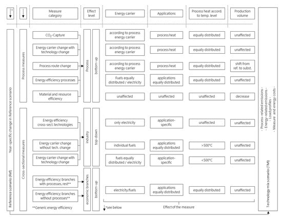
Figure 6.
Functionality of the evaluation module in the technology mix module.
Figure 1 shows the evaluations of the model calculations based on the reference scenario towards the technology mix scenario from left to right. The individual measure categories are shown in the figure according to the different evaluation methods. In order to explain the figure in more detail, an exemplary evaluation is first carried out using energy efficiency technologies. The technology mix scenario is based on the change in the reference scenario. The measure category “Energy efficiency processes” has an effect at process level. Consequently, a bottom-up approach is used. At the economic branch level, the efficiency measure only affects electricity and fuel consumption. No further distinction is made between energy carriers. Since the effect on different applications such as mechanical energy or process heat is not included in efficiency measures in the model, the measure is equally distributed across all applications. This also applies to the temperature distribution defined in the process heat. Production quantities are not affected by efficiency measures.
In order to use generic and homogeneous functions in the evaluation module, the heterogeneous GHG abatement measures must always act at the parameter level with the highest degree of detail. Therefore, a process-specific GHG abatement measure does not affect the total energy consumption of the industry, but the energy consumption of the respective process. Subsequently, the changed energy consumption is aggregated bottom-up to a higher parameter level. The effect of the measure categories on the respective parameter level is also shown in Figure 6.
In order to build on the reference scenario, it is necessary to clarify how to deal with the year-specific changes already made in the reference case. On the one hand, the reference change must be computed for all parameters that are affected by the measure implementation at the lowest parameter level. On the other hand, the reference change must be entered for those parameters that cannot be calculated bottom-up from the activity parameters:
- Process energy consumption and production volume (lowest parameter level of the processes)
- Energy carrier application matrix (EAM) (lowest parameter level of the economic branches)
Although GHG abatement measures also affect parameters at the industry level, their reference development need not be incorporated into the technology mix module. In the technology mix module, amended parameters at industry level are always distributed top-down to the processes, cross-sectional technologies and economic branches. Energy consumption is subsequently aggregated to higher parameter levels.
Furthermore, it must be determined how the year-specific reference change is taken into account in the technology mix module. In principle, two methods are conceivable: in the first option, the reference change has a percentage effect on the parameters of the technology mix module. Inconsistencies such as those that could arise from any negative parameters as a result of the absolute reference change are thus avoided. However, the reference change would be increasingly attenuated, because most parameters would decrease as a result of the GHG abatement measures. The percentage reference changes would be calculated increasingly on the basis of lower values in the technology mix module. For this reason, the second option, where the absolute reference change is related to the parameters of the technology mix module, is considered below. Thus, the change of the parameters in the technology mix module due to the reference change has an equi-constant distance to the change of the parameters in the reference scenario.
Regardless of the parameters, the reference change results from Equation (32). The reference change is applied to the parameters of the technology mix module according to Equation (33). In addition to the reference change, the GHG abatement measures implemented must also be taken into account:
| parameter in technology mix including reference change in t | change of parameters in reference |
| measure effect on parameter P in t |
The measure implementation is not linked to the changed parameters of the evaluation module. Therefore, it is a risk with the second option that both the reference change and the GHG abatement measures continue to be implemented even though parameters such as energy consumption or production volumes have already reached a zero value. If this problem occurs, a compensation function returns the parameters to their initial state. In the long term, however, it makes sense to include the evaluation module in the measure implementation function.
Each GHG abatement measure has an individual effect and is therefore implemented separately. Interactions of the individual measures are thus taken into account. The measure sequence previously determined based on the GHG abatement costs and measure implementation plays a decisive role in the measure effect. If, for instance, the process route changes from primary to secondary steel production before CO2-capture is used in the primary steel route, lower energy consumption and emissions from the original production process remain. The CO2-capture potential in primary steel production is reduced accordingly.
The methodology of the measure effect in the evaluation part of the technology mix module is described in detail below. Initially, the change in electricity and fuel consumption is calculated according to Equations (34) and (35):
| (MWh) absolute change of electricity in t by measure j | (MWh): absolute change of fuel in t by measure j |
| (MWh/tp | MWh/f) specific change of electricity | (MWh/ | MWh/f) specific change of fuel |
The calculation of the change in electricity and fuel consumption is different for the measure categories of process route change, energy carrier change with technology change and energy efficiency at economic branch level. For the process route change, the annual energy difference between the reference route and the substitution route is calculated. Instead of calculating the energy difference between two process routes, for the energy carrier change with technology change at process level the initial fuel distribution is compared with the target one. Equations (36) and (37) apply for both measure categories:
| (MWh): absolute change of electricity in t by measure j | (MWh): absolute change of fuel in t by measure j |
| (MWh/t): specific electricity consumption of reference or substitution | (MWh/t): specific fuel consumption of reference or substitution |
| (%): vector with percentage of fuels of reference or substitution process | |
For generic energy efficiency at the economic branch level, the annual, absolute energy savings are already available in the measure matrix. Therefore, Equations (38) and (39) apply:
| (MWh): change of electricity | (MWh): change of fuel |
Equations (34)–(39) calculate the annual change in electricity and fuel consumption. However, the measures implementation is not always connoted with decreasing electricity and fuel consumption. For example, the electrification of low-temperature heat reduces fuel consumption, but electricity consumption increases. The total energy consumption is still reduced due to the higher efficiency through electrification. The effect of the individual GHG abatement measures at parameter and parameter level depends on the respective measures category. Since production processes do not fully cover the economic branches and therefore aggregation from process to industry level is not possible, process measures affect both the electricity and fuel consumption of the process itself and the EAM of the economic branch. Furthermore, there are endogenous changes in the process production volume as a result of process route change. Accordingly, Equations (40) and (41) require a recalculation of the production volumes for the reference process (e.g., primary steel production) and the substitution process (e.g., H2-steel production). The production volume of the final product produced in Germany does not change as a result of the measure implementation:
| (t): production volume of reference route in t | (t): measure implementation amount of production route change |
| (t): production volume of substitution route in t | |
The effect on the electricity and fuel consumption of the processes is described by Equations (42)–(44). On this basis, the specific electricity and fuel consumption is also recalculated in Equations (45) and (46):
| (MWh) absolute electricity consumption of the process | (MWh/) specific electricity consumption of the process |
| (MWh) absolute fuel consumption of the process | (MWh/) specific fuel consumption of the process |
In order to implement the effect of a process measure on the EAM at economic branch level, different methods are required depending on the measure category. As long as the effect on specific energy carriers and applications is not known for some measure categories, the percentage distribution of the EAM available at time t is first calculated according to Equation (47):
| (%) percentage of element a in row I and column l | (dL) Matrix A with m times n elements |
| (div) element a of matrix in row i and column l | |
On the basis of the percentage EAM, the amended electricity and fuel consumption changes the existing applications and energy carriers according to Equations (48) and (49):
| (MWh) matrix with percentage distribution of energy carrier and applications electricity | (MWh) matrix with distribution of energy carrier and applications, fuels |
| (%) matrix with percentage distribution of EAM electricity | (%) matrix with percentage distribution of EAM fuels |
In contrast, the effect of process route changes and CO2-capture on the EAM can be determined based on the existing energy carrier distribution of the process. The process route change only affects the process heat of the EAM (see Equations (50) and (51)):
| (MWh) process heat, electricity | (MWh) vector with distribution of fuels for process heat |
| (%) vector with percentage distribution of fuels for process heat | |
Similarly, the measure category “energy carrier change with technology change” at process level only affects the process heat of the EAM. In contrast to the process route change, a target distribution for the production process with modified technology is used instead of the process difference.
The increased energy consumption due to CO2-capture only changes the process heat of the EAM. For this purpose, the changed fuel consumption is multiplied by the fuel distribution of the process in which CO2-capture is implemented (see Equation (52)). The change in electricity consumption is computed analogously to Equation (50):
| (MWh): vector with constant percentage distribution of fuels |
The process heat of the EAM is still divided by the temperature level. Where no temperature levels are available for each measure, the previously calculated process heat for process measures is distributed to the temperature levels on the basis of the existing temperature distribution for each economic branch. For this purpose, the existing percentage temperature distribution of the process heat is calculated according to Equation (47). The process heat subdivision between electricity and fuel consumption is computed as shown in Equations (53) and (54):
| (MWh) vector with distribution of power heat by temperature level, electricity | (%) vector with percentage of power heat by temperature level, electricity |
| (MWh) matrix with distribution of power heat by temperature level, fuels | (%) matrix with percentage of power heat by temperature level, fuels |
For the process route change from the primary steel route to the H2-steel route, it is also taken into account that the required hydrogen is only used in a temperature band above 500 °C.
With the exception of generic energy efficiency, the changed energy consumption is calculated top-down for the cross-sectional measures in the technology mix module. For generic energy efficiency, therefore, Equations (48) and (49) are used to compute the EAM, and Equations (53) and (54) to calculate the temperature-distributed process heat. The remaining cross-sectional measures affect the EAM at industry level. The application affected by the cross-sectional measures, is already available in the measure matrix. Accordingly, the EAM is calculated as shown in Equations (55) and (56):
| (MWh) vector with distribution of energy carriers of application x, fuels | (%) vector with percentage of EAM of applications x, fuels |
| (MWh) value of EAM of application x, electricity | |
Despite the available related applications for cross-sectional measures, the fuel change in the measure matrix is so far not distributed by energy carriers. However, it is taken into account that fossil fuels are substituted first’. Secondly the GHG abatement measures also have an effect on renewable fuels such as biomass. The measures category “efficiency of cross-sectional technologies” only affects electricity-based applications.
The distribution of process heat by temperature level at industry level is available for the measure categories “energy carrier change with technology change” and “energy carrier change without technology change” for each individual measure. The measure effects on the temperature band of the process heat is described in Equations (57) and (58):
| (MWh) power heat for temperature level x, electricity | (MWh) vector with power heat for temperature level x by energy carrier, fuels |
| (%) vector with percentage of power heat for temperature level x by energy carrier, fuels | |
Subsequently, the changed energy consumption is subdivided from industry level to economic branch level. The distribution is based on the premise that the energy carrier and application distribution of the economic branches do not change as a result of the measure implementation at industry level. In addition, the measures does not change the share of economic branches in the total industrial energy consumption.
In order to divide the changed energy consumption, resulting from the implementation of individual cross-sectional measures, in a top-down manner from industry to economic branch level the percentage share of economic branches in the total energy consumption of the EAM at industry level must first be computed (see Equation (59)). The resulting distribution of energy consumption from industry level to economic branch level is based on Equations (60) and (61):
| (MWh) EAM at branch level, old | (%) matrix with percentage of EAM at branch level based on EAM at industry level |
| (MWh) EAM at branch level, new | (MWh) EAM at industry level |
Once the cross-sectional effect of the measures is distributed across the economic branches, the changed parameters resulting from the measure implementation are available both for process measures and for cross-sectional measures at the economic branch level. Once the effect of the individual GHG abatement measure is applied, three function-based aggregation steps are carried out, for both cross-sectional and process measure categories:
- The energy carrier application matrices are aggregated from economic branch to industry level
- At economic branch as well as at industry level, the energy carrier application matrices are reduced by the dimension of the applications. Therefore, the energy consumption is aggregated by energy carrier.
- Afterwards, the energy carrier-specific vectors are aggregated to electricity, fuel and total energy consumption per economic branch and industry.
After the effect of an individual measure is applied, the new percentage distribution of the EAM and the temperature distribution of the process heat are computed at both economic branch and industry level, based on Equation (47). Additionally, based on Equation (59), the new percentage share of the economic branch-specific EAM’s in the total industrial energy consumption is also determined.
On the basis of the energy consumption in the technology mix module, the standardised, real data synthesised load profiles contained in the model are multiplied by the energy-carrier-specific consumption at economic branch level (see Equation (62)). The load profiles are differentiated once by energy carrier and once by application “space heating and hot water” and the remaining applications [32]. Finally, the load profiles are aggregated from economic branch level to industry level:
| (MWh) load profile according to energy carrier branch, and application | (MWh) consumption according to energy carrier branch and application |
| (%/100) standardised load profile of branch b | |
In addition, the model distinguishes between energy-and process-related emissions. In industry, energy-related emissions are caused mainly by the conversion of energy sources to generate electricity and heat. GHG abatement measures that reduce electricity and fuel consumption, consequently also reduce energy-related emissions. By contrast, process-related emissions do not result from the conversion of energy sources into other forms of energy, but are emitted by the operation of a facility or by process-related conversion steps of goods or materials used in production.
In SmInd, there are currently two options available for reducing process-related emissions: process route change and CO2-capture. When switching from primary to H2-steel, for example, the process-related emissions are significantly reduced, because the direct reduction of iron oxide with hydrogen results in significantly lower process-related emissions. Process emission factors are used to compute the process-related emissions. The use of CO2-capture in the production process usually increases both electricity and fuel consumption [22]. Initially, the utilisation of CO2-capture results in additional energy-related emissions. However, some of the additional direct energy-related emissions can in turn be reduced by CO2-capture, depending on the capture rate. In addition, CO2-capture also reduces process-related emissions, depending on the capture rate. The captured emissions are calculated in SmInd according to Equations (63)–(65):
| (tCO2) additional capture through increased energy consumption | (tCO2) capture of process-related emissions |
| (tCO2) capture of energy-related emissions according to fuel | (%) percentage fuels of process p |
| (MWh/) specific energy consumption of process p | MICC,k,p () implementation amount of carbon capture of process p |
| (a) actual time step | (a) initial year |
| (%) carbon capture rate | |
The total energy-related emissions in the technology mix module in SmInd are equal to the product of the final energy consumption and the energy carrier-specific emission factor. The resulting emissions are abated by the captured energy-related CO2 emissions. The calculation methodology applies in an analogous way for process, economic branch and industry level, based on Equation (66). The process-related emissions at process level are calculated in the technology mix module according to Equation (67):
| (tCO2) energy-related emissions | (dL) number of fuels |
| (MWh) final energy consumption of energy carrier ec | () production volume process p |
| (tCO2) process-related emissions | |
The change in process-related emissions due to the process route change is already included in the changed production volume and the process-specific emission factor. If the production volume decreases as a result of the process route change, the mathematical product of the production volume and the process-specific emission factor also decreases.
The process-related emissions at economic branch level are not implied by the process-related emissions at process level and therefore cannot be determined bottom-up via activity parameters. Hence, according to (68), the measure effect at process level is taken into account for the calculation of process-related emissions at economic branch level:
| () production volume of process p after measure implementation | () production volume of process p before measure implementation |
| (tCO2) process-related emissions, branch level | |
The changed energy costs resulting from measures implementation are computed according to Equation (68). The energy carrier precise energy consumption at economic branch level is multiplied by the specific energy carrier prices. The economic branch-specific energy costs are subsequently aggregated to industry level. Finally, several modules aggregate energy consumption, load profiles, energy-and process-related emissions as well as energy carrier and measure costs to a higher parameter level in the model.
2.6. Modelling Parameter and Description of the Scenario
Technology Mix Industry (TMI) combines GHG abatement measures in a consistent industrial energy and climate scenario. In the scenario, interactions between the small-scale GHG abatement measures are taken into account. A CO2-abatement target in the industry sector is not included in the TMI scenario. Table 1 summarises the general data of the TMI.

Table 1.
Overview scenario Technology Mix Industry (TMI).
In the TMI scenario, model calculations are conducted annually between 2015 and 2050, with energy consumption and emissions being calculated annually on an hourly basis using synthetic load profiles. The implementation of GHG abatement measures is not conducted on the basis of a cost-minimising target function. However, the GHG abatement measures are prioritised by abatement costs and replaced over natural reinvestment cycles dependent on the facility lifetime. The additional implementation of measures in the TMI scenario begins in 2021. The model has an macroeconomic perspective. Accordingly, neither an additional CO2 price nor other taxes or levies are taken into account in the industry sector. The assumed interest rate for investments is 3.5% without distinction between equity and debt capital. In the scenario, an unrestricted budget is predefined. Accordingly, the measures are implemented independently of their costs. CO2 capture as well as slightly increased industrial use of biomass are part of the TMI scenario. The scenario-sensitive analyses include learning curves that reduce the investments in the technology mix module. It is explicitly indicated, if learning curves are included in the evaluation.
The development of final energy consumption in the TMI scenario is determined by the implementation of additional GHG abatement measures compared to the start scenario. The categories of measures contained in Figure 4 are implemented in the TMI. These measure categories contain a total of 117 individual measures for industrial GHG abatement, which are combined in the TMI scenario.
The data of the measures used in the TMI scenario are available in [46,47]. Table 2 shows the mean of the input data for each measure category. Furthermore, the initial and end year are included for each measure category. However, individual GHG abatement measures of the respective measure category can also be fully implemented before 2050 (latest end year). In the following section, the individual measure categories and the most important associated individual measures for GHG abatement in the scenario are briefly described.
Table 2.
Characteristic parameters and values by measure category in TMI.
2.6.1. Energy Efficiency Processes
For the process-specific increase in energy efficiency, a distinction is made between the internal use of waste heat, the conversion of waste heat back into electricity (e.g., Organic Rankine Cycle) and the increase of general process efficiency, e.g., through improved process control and monitoring. The additional diffusion of efficiency technologies to increase process efficiency in the TMI scenario begins in 2021. The included process-specific efficiency measures are almost completely implemented by 2050 with a natural replacement rate. The scenario contains 71 process efficiency measures with an average natural replacement rate of 6% per year. In addition, the average application factor is 56%.
2.6.2. Energy Efficiency Cross-Sectional Technologies
In addition to process-specific efficiency, efficient cross-sectional technologies and their efficient use and operation are key drivers for reducing final energy consumption in the TMI scenario. These include the increasingly efficient supply of air conditioning, space heating and hot water, compressed air, pumps, information and communication technology, other mechanical energy, and lighting. Increasing efficiency of power-based cross-sectional technologies is implemented in the TMI scenario between 2021 and 2050.
2.6.3. Generic Energy efficiency
Due to a strongly heterogeneous German industry [10], the complete modelling of more efficient energy utilisation via individual GHG abatement measures is not practicable. Accordingly, the change in the efficiency of the remaining energy consumption, which is not reflected by the 22 energy-and emission-intensive processes in SmInd, is represented by generic energy efficiency measures. The average replacement rate for generic efficiency measures is, based on energy efficiency at process level, also 6% per year.
2.6.4. Process Route Change
The process route change measure category summarises process-specific GHG abatement measures that involve a change away from the classic production process. The process route change is not necessarily accompanied by a reduction in the final energy consumption, but usually promises a change to climate-neutral energy sources. In the TMI scenario, the glass industry increasingly deviates from the classic production processes of hollow glass and flat glass production to switch to electricity based glass production. Firstly, the final energy consumption can be significantly reduced through increased electrical efficiency compared to the use of gas. Secondly, instead of the fossil fuel natural gas, electricity is used, which is almost climate-neutral if renewables are used for electricity generation. Additionally, in the TMI scenario, primary steel production using blast furnaces is substituted by alternative processes. For this purpose, H2-based direct reduction with a subsequent melting process is used and the proportion of recycled steel (secondary steel production) is increased.
2.6.5. Energy Carrier Change with Technology Change—Cross-Sectional Measure
In the case of emission-free electricity, GHG abatement is also achieved by electrifying industrial low-temperature heat. Proven technologies such as the industrial heat pump and the electrode heating boiler are available in an industrial temperature range of up to 250 °C. This involves a technology change from fuel-based to electricity-based heat generation plants and the related infrastructure. In contrast to the process route change, the production process itself does not change. The electrification of low-temperature heat in a temperature range below 100 °C Space heating and hot water as well as process heat below 100 °C by use of the industrial heat pump offers a high potential for reducing fuel consumption, while electricity consumption hardly increases.
2.6.6. Energy Carrier Change with Technology Change—Process Measure
In addition to low-temperature electrification, a partial energy carrier change with technology change in the cement and lime industry is carried out. By changing the solid fuel burner to a multi-fuel one, the use of gaseous fuels becomes possible. As many cement and lime kilns already have a multi-fuel burner installed, the remaining application potential is assumed to be only 20%.
2.6.7. Energy Carrier Change without Technology Change
A change of energy carrier without a technology change requires that industrial processes can be operated unchanged even if the energy carrier is changed. This is the case, for example, with similar properties of reference and substitute fuels. The substitution of natural gas by synthetic methane therefore does not require any technology change and therefore no additional investment. For this measures category, the energy consumption of the process does not change. However, emissions are reduced if synthetic methane is produced from renewable carbon sources and almost emission-free electricity. In addition to replacing natural gas with synthetic methane, coal is increasingly being substituted by solid biomass in the TMI scenario. It is assumed that the biomass is raised to a similar energy level to coal through additional conversion steps in advance. Biocoal with similar properties is already available on the market [48,49]. Thus, no technology change is necessary for the energy carrier change from coal to biomass. Therefore, the electricity and fuel consumption does not change with this GHG abatement measure either.
2.6.8. CO2-Capture
CO2-capture in industry is in particular an important instrument for reducing process-related emissions, such as those generated during the deacidification of limestone in the cement industry [39]. In addition to the cement industry, the steel industry is a not negligible emitter of process-related emissions, which are mainly caused by the reduction of ferric oxide to iron by coke in the blast furnace route [50]. In the TMI scenario, CO2-capture is conducted for the cement and steel industries. The use of carbon capture in the model is possible from 2030.
3. Results and Discussion
Figure 7 shows the difference in industrial final energy consumption between the reference and the TMI scenario in 2050, unbundled by energy carrier and measure category. The development of energy consumption between 2020 and 2050 of the reference as well as the TMI scenario is also available in Appendix C, Figure A1. In order to better classify the results in the technology mix module based on the developed methods, a comparison with the studies [4,5,22,25] is possible.
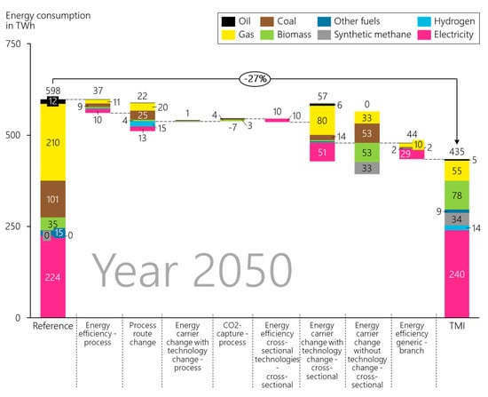
Figure 7.
Difference in industry’s final energy consumption between Reference and TMI-Scenario.
Due to additional electrical consumers (power-to-heat) in industrial heat generation in the low-temperature range and the partial electrification of appropriate high-temperature processes, despite significant efficiency gains, electricity consumption rises by 16 TWh in the TMI scenario compared to the reference scenario. The remaining coal consumption is also completely substituted by biomass in 2050. Mainly due to the process route change from blast furnace route to H2-steel production in the steel industry, an industrial hydrogen consumption of about 14 TWh results. Total energy consumption decreases from 598 TWh in the reference scenario by 27% (163 TWh) to 435 TWh in the TMI scenario in 2050. This is mainly due to efficiency gains of about 90 TWh from process and cross-sectional efficiency. The efficiency increase in energy and emission-intensive industrial processes such as cement, steel and aluminium production reduce the final energy consumption by around 37 TWh. As a result of the increasing efficiency of electricity-based cross-sectional technologies, the final energy consumption decreases by just under 10 TWh in the TMI scenario between 2021 and 2050. Due to the generic increase in efficiency, electricity and fuel consumption decrease by 29 TWh and 15 TWh respectively between 2021 and 2050. Consequently, including generic efficiency, the final total energy consumption decreases by 44 TWh. The reduction in electricity and fuel consumption is counteracted, among other things, by the use of CO2-capture, which results primarily in an increased fuel consumption of around 7 TWh in 2050 compared to the reference scenario.
Although the process route change reduces coal, gas and oil consumption, it also increases hydrogen and electricity consumption. However, this measures category reduces energy consumption overall by 22 TWh compared to the reference scenario. In the year 2045, about 4.8 million t. electric hollow glass and 2 mill. t of electric flat glass are produced in the TMI scenario. As a result, glass in Germany is produced entirely using electricity-based processes in 2045 in the TMI scenario. The complete process route change reduces gas consumption by around 8 TWh in the TMI scenario. Due to the lower specific energy consumption in electricity-based glass manufacturing, the process route change involves an additional electrical consumption of only 5 TWh. In addition, compared to the reference scenario, approximately 10 mill. t of additional secondary steel and H2-steel are produced in 2050 in order to fulfil the forecast steel production of approximately 32 mill. t in Germany [25] in 2050. The alternative steel routes increase the electricity consumption by approximately 8 TWh by 2050. The production of H2-based steel requires an additional 13 TWh of hydrogen in 2050 compared to the reference scenario. In contrast to secondary steel production, the H2-steel route is not necessarily associated with a decline in final energy consumption. Due to increased efficiency in the blast furnace route, the cumulated energy difference between the blast furnace route and the H2-steel production in the TMI scenario becomes negative. This is also based on the fact, that efficiency potentials in H2-steel production, based on experience in process control, can only be exploited after 2050. Accordingly, the conversion of the blast furnace route to the H2-route in the TMI scenario does not reduce the final energy consumption by 2050. Nevertheless, GHG emissions are significantly reduced by the process route change, because in contrast to the blast furnace route, there are hardly any process-related emissions left in H2-steel production. In addition, energy-related emissions are reduced by the substitution of coke by hydrogen, gas and electricity (see Figure 7).
The electrification of low-temperature heat in a temperature band below 100 °C by use of industrial heat pumps results in a reduction of fuel consumption of 78 TWh and an additional electricity consumption of 22 TWh in the TMI scenario. Electrification and the associated integration of renewable heat sources can therefore increase efficiency by a factor of 3.5. In 2050, space heating, hot water and low-temperature process heat in the TMI scenario are provided almost entirely by electrical energy. Only individual barriers at some factories prevent the complete electrification of the applications in the scenario. The use of the electrode boiler in a temperature band between 100 and 250 °C leads to a reduction in fuel consumption of 30 TWh and an increase in electricity consumption of 29 TWh in the TMI scenario compared to the reference scenario in 2050. The increase in efficiency decreases with rising temperature levels, as environmental heat or geothermal energy can only be integrated to a lesser extent at high temperatures [51].
By using the energy carrier change with technology change in the cement and lime industry, fuel consumption can be reduced by about 0.6 TWh due to the more efficient use of gas. In addition, synthetic methane will increasingly be used instead of gas for firing the facilities in the new multi-fuel burners in the TMI scenario. In 2050, the rotary kilns are fired largely with synthetic methane and alternative fuels.
By changing energy carriers without changing technology, coal and gas are substituted by biomass and synthetic methane respectively. No changes in investments are expected; only the variable operating costs change as a result of this measures category. In total, slightly more than 50 TWh of coal and 30 TWh natural gas are substituted by biomass and synthetic methane respectively.
Figure 8 shows the ramp-up of the individual measure categories (left). Furthermore, the figure compares the ramp-up of all process efficiency measures implemented in the model (71) (right). Figure 8 underlines that the energy savings achieved in TMI scenario, compared to the reference scenario, require the full implementation of almost all GHG abatement measures in the model. Only individual efficiency measures, CO2-capture and energy carrier change with technology change at process level still have GHG abatement potentials after 2050. However, it is also clear that the ramp-up of measures must begin as soon as possible in order to achieve the computed energy and emission savings by 2050. The left diagram shows the individual modelling of efficiency measures in SmInd. Figure 8 highlights that individual efficiency measures are above and below the scenario average (black dotted line) of the measure ramp-up with regard to their reinvestment cycle (replacement rate).
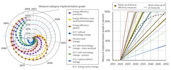
Figure 8.
GHG abatement measure ramp-up of the different categories (left) and ramp-up of individual small-scale efficiency measures (right).
Figure 9 illustrates the effect of the measure ramp-up on energy and process-related emissions and the associated change in emissions between the reference and TMI scenarios in 2050, specified by measure category. The emissions development between 2020 and 2050 of the reference and TMI scenario is also available in Appendix C, Figure A4.
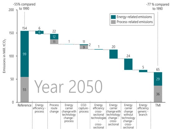
Figure 9.
Emission difference between reference and TMI scenario according to category in 2050.
Overall, in 2050 there is an emissions saving of about 90 mill. tCO2 in the TMI compared to the reference scenario. Even in the reference case, the emissions of German industry fall by 55% compared to 1990. In the TMI scenario, the additional savings result in a 77% emissions reduction compared to 1990. Further abatement potential for energy-related emissions lies in the substitution of natural gas and oil by indirect or direct electrification. Although energy efficiency measures promise to reduce electricity consumption, they hardly (still) contribute to reducing CO2-emissions due to the low electricity emission factor in 2050. Also due to the low electricity emission factor of 60 g/kWh on average in 2050, low-temperature electrification (energy carrier change with technology change—cross section) is responsible for a large part of the emission abatement between reference and TMI scenario.
The abatement of process-related emissions has proven to be particularly difficult in industry. The process route changes in the steel industry from the blast furnace route to the H2-and recycling route respectively result in a process-related emission abatement of 11 mill. t of CO2. CO2-capture in the cement industry also promises a reduction in process-related emissions of 9 mill. tCO2 in 2050. Despite the increased electricity and fuel consumption caused by the additional required energy to capture CO2 in the production process (see Figure 7), additional energy-related emissions of around 2 mill. tCO2 can be avoided in 2050. Although the use of multi-fuel burners in the cement industry involves the conversion to climate-neutral fuels such as gas, in 2050 it only results in a CO2 abatement of around one million tonnes. This is primarily because of the potential limit reflected in the application factor, because around 80% of rotary kilns in Germany are already equipped with multi-fuel burners. The use of biomass and synthetic methane without technology change results in a high abatement of emissions, as mainly emission-intensive coal and natural gas are replaced by emission-free fuels.
The analysis reveals that the emission savings can be attributed to four large GHG abatement clusters. Figure 10 summarises the clusters and their share in the total emission abatement as well as further important TMI scenario results.
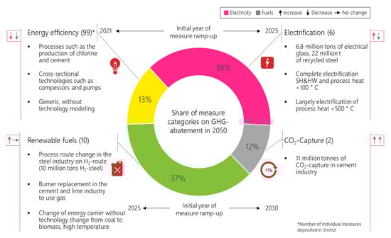
Figure 10.
The four major levers for reducing GHG emissions in industry.
Figure 10 illustrates that especially electrification and the use of renewable fuels offer great potential for abating GHG emissions in the TMI scenario. With a share of almost 40% each, further research is needed to focus on these two abatement options. Nevertheless, energy efficiency is also an option that should not be neglected because of the limited area potentially available for renewable energy generation, so that pressure on the supply sector is reduced.
Figure 11 shows the electricity costs course in the reference and TMI scenarios as a function of energy consumption changes.
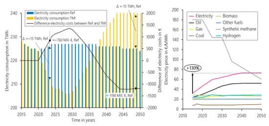
Figure 11.
Left: Development of electricity consumption in the Ref and TMI scenarios and difference in electricity costs between them. Right: Endogenic energy prices of ISAaR used in both scenarios.
Apart from electricity consumption alone in 2023 and 2049, there are also large differences in electricity costs. The additional consumption of 15 TWh in the reference scenario related to the implementation of efficiency measures from 2021 in the TMI scenario, on the one hand, results in additional costs of €760 mill. In the TMI scenario, on the other hand, the same electricity difference results in additional costs of around €1190 mill. in 2049. This is based on increasing electricity prices between 2015 and 2050 (130%). By multiplying the energy prices in Table A2 by the energy consumption in Figure A1, the absolute energy costs of the two scenarios in 2050 can be calculated.
Figure 12 shows the total costs of the TMI scenario divided by investment, fixed operating costs and energy costs per year (left bar per year). The right bar reflects the total costs, taking learning effects into account.
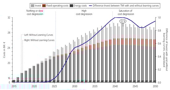
Figure 12.
Cost of the TMI scenario without (left bar) and with (right bar) learning curves differentiated according to investment, fixed operating and energy costs, additionally standardised difference between investment with and without learning curves (purple line).
Figure 12 illustrates that learning curves only affect investment. Therefore, learning effects are only taken into account in the production and provision of technologies used to abate greenhouse gases. Effects that influence fixed operating costs are not included. The blue line shows the standardised cost difference between the investments with and without learning effects. Three phases can be outlined in the course of the inverted logistic growth:
- Cost degression initially rises slowly between 2021 and 2025
- Strongest cost degression in the middle section between 2025 and 2040
- Cost degression increases moderately; no further degression of investment can be observed in 2040. The subsequent decrease of the curve after 2043 can be explained by the complete repayment of the first annuity investments recorded in the balance sheet from the initial years of measure implementation.
The largest difference in investment between the TMI scenario with and without learning curves can be observed in 2040 (EUR 826 million). In 2050, the cost difference is still €780 million. Cumulatively, investment is reduced by EUR 15 billion between 2020 and 2050 by taking learning curves into account in the TMI.
In addition to the evaluation of measure categories, the small-scale modelling of individual measures also makes it possible to evaluate individual GHG abatement measures. As it is not practicable to evaluate all 117 individual measures, the process route changes from the blast furnace route to the H2 and secondary steel routes are evaluated as an example.
Figure 13 shows the ramp-up of GHG abatement measures according to the degree of measure implementation and the production volume of individual process routes for steel production.
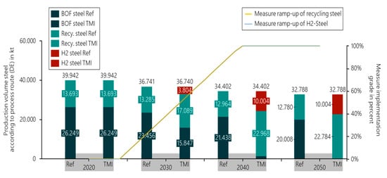
Figure 13.
Production volume of steel production according to process route and start of production of process route changes in the steel industry, 2020–2050, BOF: Blast Oxygen Furnace.
Total exogenous steel production in Germany decreases by 7 mill. t by 2050 [22,25]. Figure 13 illustrates that the ramp-up of the process route change in the TMI scenario begin between 2020 and 2030. In the TMI scenario, steel production is completely shifted to the secondary and H2-steel routes by 2040.
Figure 14 shows the energy carrier-specific change in energy consumption as a result of the alternative process routes. The changes in energy and process-related emissions are also listed (secondary axis).
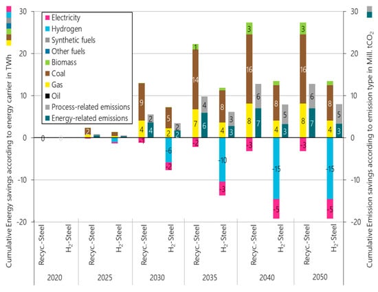
Figure 14.
Changes in energy and emissions as a result of process route changes, lower/higher energy consumption compared to Reference is positive/negative, lower/higher emissions compared to Reference are positive/negative.
Due to the process route change from blast furnace-to secondary steel both energy and emission savings are significantly higher compared to the process route change from blast furnace-to H2-steel.
On the one hand, the production of secondary steel requires significantly less energy than the production of H2-steel. The difference in energy consumption between blast furnace steel and secondary steel is correspondingly much higher. As a result, energy consumption and energy-related emissions decrease more strongly compared to the H2-route. On the other hand, the process-related emissions of the secondary steel route are significantly lower than those of the H2-steel route.
Although there is a higher process-related emission difference between blast furnace and secondary steel production, a complete shift to the secondary steel route is not possible because there is not enough scrap available worldwide [52]. Accordingly, the production of primary steel (H2-steel) in industry is still necessary. Both measures determine a significant increase in electricity consumption, which is related to the increased integration of the electric arc furnace. The H2-steel route also shows an additional consumption of 15 TWh of hydrogen. Through efficiency measures in the overall technology mix scenario, the hydrogen consumption is reduced to around 14 TWh by 2050.
Finally, Figure 15 shows the cost difference between TMI and reference scenario of the two process route changes in the steel industry. The process route changes are shown both with (left bar) and without learning curve effects (right bar). In addition, the standardised difference in investment between the implementation with and without learning curves of both measures is shown.
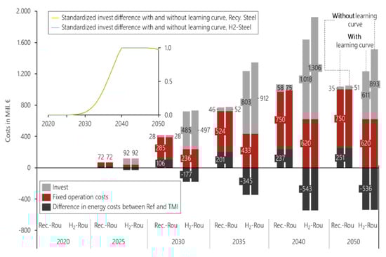
Figure 15.
Difference of the energy carrier and fixed operating costs including investment between the Reference and TMI scenarios with and without learning curves, standardised investment difference between the measure implementation with and without learning curves, 2020–2050.
In particular, the H2-route involves significantly higher investments than the secondary steel route. Accordingly, learning curve effects on absolute investment are also higher. If the standardised investment difference curves are used, the same natural reinvestment cycle of both process routes results in an almost identical curve shape. However, the fixed operating costs are significantly lower in the H2-steel route. In secondary steel production, energy carrier costs rise compared to the blast furnace route, as both electricity consumption and electricity price increase significantly in the scenario. As a result of the significantly lower hydrogen price (~28 €/MWh) compared to the electricity price (~76 €/MWh) in 2050, the energy carrier costs in the H2-steel route decrease compared to primary steel production. In 2050, secondary steel production with learning effects also incurs additional annuity costs of €341 mill. compared to the H2-route due to the lower energy costs.
4. Conclusions
In this publication, the methodological and implementation-oriented extension of the sector model industry (SmInd) with a technology mix module is presented, combining 117 individual GHG abatement measures and allowing for interactions between the individual measures. The technology mix module enables the construction of consistent technology mix scenarios in industry. Typical results of the technology mix module are evaluated not only at industry level, but also at individual measure level.
For the development of the technology mix module, the following three steps are conducted: Initially, preparatory calculations are carried out to cover the entire final energy consumption of industry through GHG abatement measures. In addition to the already existing measure categories [1,32], an implementation methodology of four measure categories is developed: energy efficiency of the cross-sectional technologies, material and resource efficiency, the energy carrier change without technology change from coal to biomass and generic energy efficiency. The GHG abatement measures are incorporated into an overall measure matrix containing all relevant parameters. As a result of the measure matrix it is possible to determine year-specific initial and end years for the implementation of individual measures.
Depending on the measure category, a methodology for the combination of individual GHG abatement measures is under development, considering both, the implementation and the effect of the individual measures. For the year-specific ranking of GHG abatement measures, year-dependent, static GHG abatement costs are calculated. Subsequently, the overall measure matrix is prioritised according to these costs. In this context, annuity investments, non-annuity energy costs and fixed operating costs as well as year-specific emission factors are used. The implementation of the measures in the model is currently related to two restrictions: the complete implementation of the measures and a specified monetary budget. The complete implementation of a measure is determined by the measure’s potential and natural reinvestment cycles, which depend on the technology lifetime [32]. In addition, the technology mix module offers the possibility of parameterising the measure ramp-up using any mathematical function on the basis of real data and thus simulating a non-linear measure ramp-up. The budget restriction enables the limitation of the measure’s implementation according to measure costs. Both fixed operating costs and investments are included. To calculate the investments, the model offers an additional option of learning effects implementation. The learning curves are oriented to parameterised, inverted logistic growth curves.
Effects of the measures on the output parameters of the technology mix module are determined in the evaluation module. In order to use generic and homogeneous functions in the evaluation module, the heterogeneous GHG abatement measures always affect the parameter level with the highest degree of detail. The reference change must also be taken into account. For this purpose, a methodology is developed, in which year-specific reference changes have an equi-constant effect on the parameters of the technology mix module. Interactions are taken into account by implementing the GHG abatement measures according to the previously computed GHG abatement costs ranking. Afterwards, the parameters are aggregated from lower to higher parameter levels.
The developed methodology for combining small-scale GHG abatement measures in an industrial technology mix module leads to a technology mix scenario (TMI) with typical results. Compared to the reference scenario, industrial final energy consumption in the TMI falls by 163 TWh in 2050. Compared to 2020, energy consumption in the TMI scenario decreases by 256 TWh. In the TMI scenario, the energy and process-related GHG emissions of industry in Germany decrease by 90 mill. tCO2 to 65 mill tCO2 in 2050 compared to the reference scenario. Compared to 1990 (283 mill. tCO2), an emission reduction of 77% is achieved in the TMI scenario (reference: 55%). This requires a ramp-up of the measures as soon as possible, as otherwise the industrial GHG abatement measures cannot be fully implemented by 2050 on the basis of natural reinvestment cycles. Due to its higher efficiency, the electrification of heat contributes particularly to the reduction of energy consumption and emissions. Renewable fuels have the potential to reduce both energy and process-related industrial emissions. In addition to electrification and the use of renewable fuels, energy efficiency and CO2-capture contribute also, but to a lesser extent, to GHG abatement in industry. If, in addition, inverted logistic growth curves for mapping learning effects in the development of climate protection technologies are taken into account, investment expenditure falls considerably in the context of the industrial energy transition (€15 bill. between 2020 and 2050 in the TMI). The fixed operating costs do not change, as the complexity of estimating the learning effect on operating processes in industry goes beyond the analysis objective of this paper.
The evaluation of individual small-scale GHG abatement measures using the example of process route changes in the steel industry shows that the blast furnace route in the TMI is completely replaced by the H2-and secondary routes in 2040. About 10 mill. t. of additional secondary and H2-steel are produced in 2050. Energy analyses at the level of individual measures show that coal and natural gas are predominantly replaced by electricity and hydrogen in the steel industry. Energy and process-related emissions are abated considerably more by the change of process route to secondary steel production than by the switch to H2-steel. The availability of scrap in 2050 limits the potential of secondary steel. Despite higher investments and fixed operating costs, the total costs of H2-steel production are significantly lower due to high electricity and low H2-prices compared to secondary steel production in 2050. The low hydrogen costs result from the fact that hydrogen production in the supply sector is predominantly based on natural gas and steam reforming respectively in the scenarios. The prices for renewable-energy-based hydrogen would probably be significantly higher (currently between 150 €/MWh and 200 €/MWh) [53,54,55].
The methodology enables the simulation of industrial transformation using detailed technology mix paths. Thus, as a result of the technology mix module in SmInd it is possible to support political decision-making and an efficient transition to greenhouse gas neutral industry [14]. The results show the implied transformation speed on the basis of natural reinvestment cycles. Effects of transformation and transformation speed in the sector become visible through industrial energy consumption and emissions. Despite the implementation of ambitious GHG abatement measures, the industrial energy transition in the scenario only achieves a GHG abatement of 77% in 2050 compared to 1990. Accordingly, much greater efforts are necessary in industry than implied in the TMI scenario. Industrial companies in Germany must prepare themselves for significantly greater efforts along the industrial transition path. In particular, support and openness are necessary for the development and the implementation of technologies that significantly reduce process-related emissions in the industry.
Despite the comprehensive methodology for small-scale modelling of GHG abatement measures in the industry, there are limitations in the simulation model that must be addressed in the future. In the model, the measures are partly linked with deterministic assumptions. For example, biomass is defined as a substitute for coal. A market decision regarding the substitution fuel on the basis of energy carrier prices would be conceivable in order to increase the degree of freedom of the model. A first step has already been taken through measures implementation based on GHG abatement costs. However, measure implementation according to static GHG abatement costs also entails false incentives: with the decrease in the electricity emission factor, the abatement costs for efficiency measures increase intensively. Regarding GHG abatement costs, it is therefore less worthwhile to increase efficiency. However, reduced efficiency increases energy carrier prices, as increased energy demand leads overall to higher prices in the supply sector. This would, in turn, reduce the abatement costs for the efficiency measure, as the energy saving leads to a higher reduction in energy costs. However, energy prices and emission factors for the observation period are determined exogenously by the supply sector. An increasingly intensive interaction with the supply sector is necessary to take the changed energy demand of the final energy sectors into account and to calculate new emission factors and energy prices. An annual rolling principle would make energy consumption changes in industry visible in the supply sector. Accordingly, new energy carrier prices and emission factors could be determined on the basis of the changing energy demand in the supply sector. Furthermore, data on the effects of individual GHG abatement measures are also not considered in detail in the model. Missing temperature levels as well as the fuel distribution of individual GHG abatement measures also affect the results. On the one hand, temperature-distributed process heat consumption of the energy and emission-intensive processes could be a remedy. A fuel subdivision of the GHG abatement measures, on the other hand, is difficult to collect due to the lack of industrial data. However, if an increase in the detail level of the modelling does not provide any significant added value, an extension should not be conducted. In particular, the GHG abatement measures for electrification and the use of renewable fuels have considerable GHG abatement potential. Accordingly, it would make sense to increase their level of detail, whereas the small-scale modelling of efficiency measures promises less added value. As the measure implementation is not linked to the amended parameters of the evaluation module, there is a risk that the parameter change continues to be implemented even though parameters such as energy consumption or production volumes have already reached a zero value. If this problem occurs, a compensation function returns the parameters to their initial state. In the long term, however, the evaluation module should be integrated into the measure implementation module.
In contrast to other scenarios that calculate or define endogenous or exogenous transformation paths, the implementation speed of the measures in the TMI scenario is not bound to a given level of climate ambition. Accordingly, the integration of a CO2-target into the measures implementation is already being processed. Two concrete options are conceived: on the one hand, a limit is set with regard to GHG abatement costs in connection with a GHG abatement target. Measures are only implemented as long as the GHG abatement target requires. On the other hand, the second option offers increased degrees of freedom for the model by setting year-specific GHG abatement targets. With this option, the model can freely decide when and to what extent the GHG abatement measures are to be applied as long as the CO2 reduction is achieved in the target year. With this option it is also possible to specify the objective by using accumulated total emissions as target parameters. Restrictions include, for example, the limited annual ramp-up of measures or cost parameters. Both options should be feasible with and without optimisation. The linear optimisation basis is a cost function that calculates the combination of measures with minimum costs and a given CO2-level. In order to enable calculations at company level as well, the measures implementation should continue to be taken from a macroeconomic to a microeconomic perspective, including taxes and levies. A differentiation of the interest rate with regard to debt and equity capital and the typical amortisation period of industrial factories is also envisaged [1].
While considerable attention is paid to defossilising the supply, transport and household sectors, the understanding of how greenhouse gases can be reduced in the industry sector is lagging behind [1,2,3]. Today, German politics and society are already targeting climate neutrality and, therefore, an almost complete cross-sector abatement of greenhouse gases by 2050 [8,56]. The dynamic bottom-up modelling of GHG abatement measures in industry provides the possibility of deriving consistent transformation paths on the basis of heterogeneous, process-specific development. Thus, the developed and implemented methodology in SmInd can support strategic decision-making in politics as well as an efficient transition to a GHG neutral industry. In order to achieve the ambitious cross-sector climate targets, industry must continue to make major efforts in the future [8].
Funding
The project on which this publication is based was funded by the Federal Ministry of Education and Research (BMBF) under the funding code O3SFK300-2. The authors are fully responsible for the content of this publication.
Conflicts of Interest
The authors declare no conflict of interest. The funding authority had no role in the design, execution, interpretation, or writing of the study.
Appendix A
Table A1.
Parameters of the yearly process and economic branch comprehensive measure list.
Table A1.
Parameters of the yearly process and economic branch comprehensive measure list.
| Index | Parameter |
|---|---|
| (1) | Measure identification number |
| (2) | Electricity change |
| (3) | Fuel change |
| (4) | Application factor |
| (5) | Lifetime |
| (6) | Investment |
| (7) | Fixed operating costs |
| (8) | Measure category |
| (9) | Substitution process of process route change |
| (10) | CO2-capture rate |
| (11) | Identification number of process or cross-section on which the measure has an effect |
| (12) | Initial year measure implementation |
| (13) | End year measure implementation |
| (14) | Economic branch name, on which the measure has an effect |
| (15) | Process name on which the measure has an effect |
| (16) | Identification number substitution process of process route change |
| (17) | Identification number economic branch |
| (18) | Natural replacement rate |
| (19) | Function of replacement rate |
| (20) | Static GHG abatement costs |
| (21) | Annuity measure investment |
| (22) | Non-annuity fixed operating costs |
| (23) | Annuity measure costs |
| (24) | Yearly measure implementation amount |
| (25) | Cumulated measure implementation amount |
| (26) | Energy carrier change reference |
| (27) | Energy carrier change substitution |
Appendix B
Energy prices and Emission factors.
Table A2.
Energy prices used in the technology mix scenario.
Table A2.
Energy prices used in the technology mix scenario.
| ⦰ Energy Price (€/MWh) | ⦰ Energy Price (€/MWh) | Literature and Origin | |
|---|---|---|---|
| Energy Carrier | 2020 | 2050 | |
| Coal | 8 | 9.6 | [57] Scenario B, [25], mean of hard coal and lignite |
| Natural gas | 22.7 | 28.1 | [57] Scenario B, [25] |
| Mineral oil | 29.8 | 51.8 | Own estimation [57,58,59] |
| Biomass | 27.6 | 26.3 | Own estimation [60] |
| Other fuels | 20 | 20 | Own estimation [60] |
| District heating | 19.2 | 34.4 | Based on simulation, FFE-ISAaR, [60] |
| Electricity | 46.2 | 72.6 | Based on simulation, FFE-ISAaR, [60] |
| Hydrogen | 23.6 | 28.1 | Based on simulation, FFE-ISAaR, [60] |
| Synthetic methane gas | 180 | 60 | Based on simulation, FFE-ISAaR, [60] |
Table A3.
Emission factors used in the technology mix scenario.
Table A3.
Emission factors used in the technology mix scenario.
| ⦰ Emission Factors (tCO2/MWh) | ⦰ Energy Price (tCO2/MWh) | Literature and Origin | |
|---|---|---|---|
| Energy Carrier | 2020 | 2050 | |
| Coal | 0.347 | 0.340 | Own calculation according to [61] mean of Hard coal and lignite |
| Natural gas | 0.198 | 0.198 | [61] |
| Mineral oil | 0.277 | 0.277 | Own calculation, [61] |
| Biomass | 0 * | 0 * | Renewable carbon cycle |
| Other fuels | 0.293 | 0.293 | Own calculation, [61] |
| District heating | 0.372 | 0.161 | Based on simulation, [60] |
| Electricity | 0.367 | 0.067 | Based on simulation, [60] |
| Hydrogen | 0 | 0 | Assumption |
| Synthetic methane gas | 0 * | 0 * | Renewable carbon cycle |
* Biomass and synthetic methane are accounted for with zero emissions in the scenario despite incipient direct emissions during combustion. This is due to the assumed renewable carbon cycle for the fuels.
Appendix C
Energy Consumption over time of Technology Mix Scenario (TMI).

Figure A1.
Energy consumption by energy carrier in the Reference (left) and TMI scenarios between 2020 and 2050.

Figure A2.
Energy consumption by fuel application and energy carrier in Reference and TMI scenarios between 2020 and 2050 (SH & HW: Space Heating and Hot Water).

Figure A3.
Energy consumption of process heat by temperature level and energy carrier in Reference and TMI scenarios between 2020 and 2050.
Emissions of Technology Mix Scenario (TMI)

Figure A4.
Energy and process-related emissions in the Reference (left) and TMI scenarios between 2020 and 2050.
Appendix D

Figure A5.
Production volume of processes according to measure category process route change in Reference and TMI scenarios between 2020 and 2050.
Table A4.
Production volume of processes in Reference and TMI scenarios between 2020 and 2050.
Table A4.
Production volume of processes in Reference and TMI scenarios between 2020 and 2050.
| Reference | TMI-Scenario | |||||||
|---|---|---|---|---|---|---|---|---|
| Industrial Process | 2020 | 2030 | 2040 | 2050 | 2020 | 2030 | 2040 | 2050 |
| milk | 13,934 | 13,686 | 13,672 | 13,654 | 13,934 | 13,686 | 13,672 | 13,654 |
| paper | 22,743 | 23,028 | 23,080 | 23,668 | 22,743 | 23,028 | 23,080 | 23,668 |
| cellulose | 1299 | 1053 | 884 | 761 | 1299 | 1053 | 884 | 761 |
| wastepaper | 15,467 | 16,215 | 16,525 | 17,380 | 15,467 | 16,215 | 16,525 | 17,380 |
| steam cracking | 12,588 | 13,527 | 14,698 | 15,874 | 12,588 | 13,527 | 14,698 | 15,874 |
| polyethylene | 3070 | 3299 | 3626 | 4008 | 3070 | 3299 | 3626 | 4008 |
| methanol | 941 | 941 | 941 | 941 | 941 | 941 | 941 | 941 |
| ammonia | 3255 | 3172 | 3153 | 3142 | 3255 | 3172 | 3153 | 3142 |
| chlorine | 4703 | 4848 | 4857 | 4849 | 4703 | 4848 | 4857 | 4849 |
| high glass | 4391 | 4535 | 4675 | 4845 | 4391 | 3207 | 1133 | 0 |
| flat glass | 1819 | 1878 | 1936 | 2007 | 1819 | 1147 | 0 | 0 |
| electric hollow glass | 0 | 0 | 0 | 0 | 0 | 1328 | 3542 | 4845 |
| electric flat glass | 0 | 0 | 0 | 0 | 0 | 731 | 1936 | 2007 |
| cement | 31,104 | 30,175 | 29,541 | 28,916 | 31,104 | 30,175 | 29,541 | 28,916 |
| brick | 10,936 | 10,609 | 10,291 | 9891 | 10,936 | 10,609 | 10,291 | 9891 |
| lime | 6605 | 6513 | 6512 | 6482 | 6605 | 6513 | 6512 | 6482 |
| primary steel | 26,249 | 23,456 | 21,438 | 20,008 | 26,249 | 15,847 | 1430 | 0 |
| secondary steel | 13,693 | 13,285 | 12,964 | 12,780 | 13,693 | 17,089 | 22,968 | 22,784 |
| H2-steel | 0 | 0 | 0 | 0 | 0 | 3804 | 10,004 | 10,004 |
| primary aluminum | 439 | 381 | 349 | 323 | 439 | 381 | 349 | 323 |
| primary copper | 397 | 397 | 397 | 397 | 397 | 397 | 397 | 397 |
| secondary copper | 281 | 281 | 281 | 281 | 281 | 281 | 281 | 281 |
References
- Sektorenkopplung, T.; HÜBNER, T.; GUMINSKI, A.; VONROON, S.; PICHLMAIER, S. Modellgestützte Analyse synthetischer Brennstoffe in der Industrie bei ambitioniertem Klimaschutz; Forschungsgesellschaft für Energiewirtschaft (FfE): München, Germany, 2019. [Google Scholar]
- Loftus, P.J.; Cohen, A.M.; Long, J.C.; Jenkins, J.D. A critical review of global decarbonization scenarios: What do they tell us about feasibility? Wiley Interdiscip. Rev. Clim. Change 2015, 6, 93–112. [Google Scholar] [CrossRef]
- Edenhofer, O. Climate Change 2014 Mitigation of Climate Change – Industry; Cambridge University Press: New York, NY, USA; Cambridge, UK, 2014. [Google Scholar] [CrossRef]
- Kruse, J. dena-Leitstudie Integrierte Energiewende—Teil B; ewi Energy Research & Scenarios gGmbH: Köln, Germany, 2018. [Google Scholar]
- Gerbert, P.; Herhold, P.; Burchardt, J.; Schönberger, S.; Rechenmacher, F.; Kirchner, A.; Kemmler, A.; Wünsch, M. Klimapfade für Deutschland; The Boston Consulting Group (BCG): München, Germany, 2018. [Google Scholar]
- Köckhuber, C.; Guminski, A.; von Roon, S. Die Grenzen der Elektrifizierung—Analyse und Bewertung von Green Fuels als Ergänzung zu Strom im dekarbonisierten Energiesystem in: et—Energiewirtschaftliche Tagesfragen 67; Jg. (2017) Heft 8; etv Energieverlag GmbH: Essen, Germany, 2017. [Google Scholar]
- Klein, S.; Steinert, T.; Fricke, A.; Peschel, D. Erneuerbare Gase—ein Systemupdate der Energiewende. Berl.Enervis Energy Advis. Gmbh 2017, 13, 2017. [Google Scholar]
- Hübner, T.; Guminski, A.; Rouyrre, E.; von Roon, S. Industrie 2050: Energiewende in der Industrie. In et-Energiewirtschaftliche Tagesfragen (Ausgabe 8, 2019); etv Energieverlag GmbH: Essen, Germany, 2019. [Google Scholar]
- Hübner, T.; Regett, A.; Fattler, S.; Guminski, A.; Pichlmaier, S.; Conrad, J.; von Roon, S. Application-side merit-order-curves for synthetic fuels in the German energy system. In Proceedings of the 13th International Conference on Energy Economics and Technology 2019, Dresden, Germany, 12 April 2019. [Google Scholar]
- Hübner, T. Die Rolle synthetischer Brennstoffe zur Erreichung der klimapolitischen Ziele—Bedeutung im Jahr 2050. In BWK (Brennstoff, Wärme, Kraft)—Das Energie-Fachmagazin 10/2018; Springer-VDI-Verlag GmbH & Co. KG: Düsseldorf, Germany, 2018. [Google Scholar]
- Brunke, J.C.U. Energieeinsparpotenziale von energieintensiven Produktionsprozessen in Deutschland—Eine Analyse mit Hilfe von Energieeinsparkostenkurven. Ph.D. Thesis, Universität Stuttgart—Institut für Energiewirtschaft und Rationelle Energieanwendung, Stuttgart, Germany, 2016. [Google Scholar]
- Climate Change 2014—Synthesis Report—Contribution of Working Groups I, II and III to the Fifth Assessment Report of the Intergovernmental Panel on Climate Change; Pachauri, R.K., Meyer, L.A., Eds.; Intergovernmental Panel on Climate Change (ipcc): Geneva, Switzerland, 2014; p. 151. [Google Scholar]
- Van Sluisveld, M.; de Boer, H.; Hof, A.; van Vuuren, D.; Schneider, C.; Lechtenböhmer, S. EU Decarbonisation Scenarios for Industry; Reinvent Project Nr. 730053; PBL Netherlands Environmental Assessment Agency: Den Haag, The Netherlands; Wuppertal, Germany, 2018. [Google Scholar]
- Fleiter, T.; Rehfeldt, M.; Herbst, A.; Elsland, R.; Klingler, A.L.; Manz, P.; Eidelloth, S. A Methodology for Bottom-up Modelling of Energy Transitions in the Industry Sector: The FORECAST Model; Fraunhofer Institute for Systems and Innovation Research (ISI): Karlsruhe, Germany, 2018. [Google Scholar]
- Fleiter, T.; Rehfeldt, M.; Herbst, A.; Elsland, R.; Klingler, A.L.; Manz, P.; Eidelloth, S. A methodology for bottom-up modelling of energy transitions in the industry sector: The FORECAST model. Energy Strategy Rev. 2018, 22, 237–254. [Google Scholar] [CrossRef]
- Rehfeldt, M.; Fleiter, T. Integration Erneuerbarer Energieträger in industrielle Hochtemperaturprozesse: Technische Grenzen des Energieträgerwechsels; Fraunhofer-Institut für System- und Innovationsforschung ISI: Karlsruhe, Germany, 2017. [Google Scholar]
- Fleiter, T.; Herbst, A.; Rehfeldt, M.; Arens, M. Industrial Innovation: Pathways to deep decarbonisation of Industry—Part 2: Scenario Analysis and Pathways to Deep Decarbonisation; Fraunhofer-Institut für System- und Innovationsforschung ISI: Karlsruhe, Germany, 2019. [Google Scholar]
- Rehfeldt, M.; Globisch, J.; Fleiter, T. Fuel choice in industrial steam generation: Empirical evidence reveals technology preferences. Energy Strategy Rev. 2019, 26, 100407. [Google Scholar] [CrossRef]
- Rehfeldt, M.; Fleiter, T.; Worrell, E. Inter-fuel substitution in European industry: A random utility approach on industrial heat demand. J. Clean. Prod. 2018, 187, 98–110. [Google Scholar] [CrossRef]
- Rehfeldt, M.; Fleiter, T.; Toro, F. A Bottom-up Estimation of Heating and Cooling Demand in the European Industry. Energy Effic. 2018, 11, 1057–1082. [Google Scholar] [CrossRef]
- Repenning, J.; Hermann, H.; Emele, L.; Jörß, W.; Blanck, R.; Loreck, C.; Böttcher, H.; Ludig, S.; Dehoust, G.; Matthes, F.C.; et al. Klimaschutzszenario 2050—2. Endbericht; Öko-Institut e.V.: Berlin, Germany, 2015. [Google Scholar]
- Pfluger, B.; Tersteegen, B.; Franke, B.; Bernath, C.; Tobias, B.; Deac, G.; Elsland, R.; Tobias Fleiter, K.A.; Ragwitz, M.; Rehfeldt, M.; et al. Langfristszenarien für die Transformation des Energiesystems in Deutschland; Fraunhofer-Institut für System- und Innovationsforschung (Fraunhofer ISI): Karlsruhe, Gernmay, 2017. [Google Scholar]
- Guminski, A.; Hübner, T.; Rouyrre, E.; Roon, S.V.; Schimmel, M.; Achtelik, C.; Rhiemeier, J.M.; Fahl, U.; Bailey, I. Energiewende in der Industrie: Potenziale und Wechselwirkungen mit dem Energiesektor; FfE: München, Germany, 2019. [Google Scholar]
- Kube, M.; Schimmel, M.; Rhiemeier, J.M.; Barckhausen, A.; Fehr, J.; Büttner, S. Marktverfügbare Innovationen mit hoher Relevanz für die Energieeffizienz in der Industrie; Ecofys: Berlin, Germany, 2017. [Google Scholar]
- Schlesinger, M.; Lindenberger, D.; Lutz, C. Entwicklung der Energiemärkte—Energiereferenzprognose—Projekt Nr. 57/12—Studie im Auftrag des Bundesministeriums für Wirtschaft und Technologie; Bundesministerium für Wirtschaft und Technologie (BMWi): Berlin, Germany, 2014. [Google Scholar]
- Janzen, F.; Witte, K. Weltwirtschaftsmodell View; Prognos AG: Basel, Switzerland, 2019; Available online: https://www.prognos.com/publikationen/prognos-economic-outlook-r/modell-view-r/ (accessed on 24 September 2019).
- Primes Model Version 2018—Detailed Model Description; E3M-Lab, National Technical University of Athens: Athens, Greece, 2019.
- Capros, P.; De Vita, A.; Tasios, N.; Siskos, P.; Kannavou, M.; Petropoulos, A.; Evangelopoulou, S.; Zampara, M.; Papadopoulos, D.; Nakos, C.; et al. EU Reference Scenario 2016—Energy, transport and GHG emissions Trends to 2050; Europäische Kommission: Brüssel, Belgium, 2016. [Google Scholar]
- Schneider, C.; Lechtenböhmer, S.; Samadi, S. Risks and opportunities associated with decarbonising Rotterdam’s industrial cluster. In Environmental Innovation and Societal Transitions 05/2019; Wuppertal Institute for Climate: Wuppertal, Germany, 2019. [Google Scholar] [CrossRef]
- Lorenczik, S.; Gierkink, M.; Schmidt, L.; Hennes, O. Kosteneffiziente Umsetzung der Sektorenkopplung; ewi Energy Research & Scenarios GmbH: Köln, Germany, 2018. [Google Scholar]
- Hecking, H.; Hintermayer, M.; Lencz, D.; Wagner, J. Energiemarkt 2030 und 2050—Der Beitrag von Gas- und Wärmeinfrastruktur zu einer effizienten CO2-Minderung; ewi Energy Research & Scenarios gGmbH: Köln, Germany, 2017. [Google Scholar]
- Guminski, A.; Hübner, T.; Gruber, A.; von Roon, S. Model based Evaluation of Industrial Greenhouse Gas Abatement Measures; Forschungsgesellschaft für Energiewirtschaft mbH: München, Deutschland, 2019. [Google Scholar]
- Rohde, C. Erstellung von Anwendungsbilanzen für die Jahre 2013 bis 2015 mit Aktualisierung der Anwendungsbilanzen der Jahre 2009 bis 2012; Fraunhofer-Institut für System- und Innovationsforschung (ISI): Karlsruhe, Germany, 2016. [Google Scholar]
- BMWi. Energiedaten: Gesamtausgabe; BMWi: Berlin, Germany, 2018. [Google Scholar]
- Unger, H.; Wagner, H.J. Validierung und kommunale Disaggregierung des Expertensystems HERAKLES—Abschlussbericht zum Vorhaben 258 114 98; Lehrstuhl für Energiesysteme und Energiewirtschaft, Ruhr-Universität Bochum (LEE): Bochum, Germany, 2002. [Google Scholar]
- Otto, A.; Robinius, M.; Grube, T.; Schiebahn, S.; Praktiknjo, A.; Stolten, D. Power-to-Steel—Reducing CO2 through the Integration of Renewable Energy and Hydrogen into the German Steel Industry. Energies 2017, 10, 451. [Google Scholar] [CrossRef]
- Energiebilanz der Bundesrepublik Deutschland 2015; AG Energiebilanzen e.V.: Berlin, Germany, 2016; Available online: ps://ag-energiebilanzen.de/7-0-Bilanzen-1990-2016.html (accessed on 26 July 2017).
- Verein Deutscher Zementwerke e.V. Zementindustrie in Deutschland 2016—Zahlen und Daten; Verein Deutscher Zementwerke e.V.: Düsseldorf, Germany, 2016. [Google Scholar]
- Umweltdaten der Deutschen Zementindustrie; Verein Deutscher Zementwerke e.V.: Düsseldorf, Germany, 2015.
- Fleiter, T.; Schlomann, B.; Eichhammer, W. Energieverbrauch und CO2-Emissionen industrieller Prozesstechnologien—Einsparpotentiale, Hemmnisse und Instrumente; ISI Schriftenreihe “Innovationspotentiale”; Fraunhofer-Institut für Systemtechnik und Innovationsforschung (Fraunhofer ISI): Stuttgart, Germany, 2013. [Google Scholar]
- Die Klimavorsorgeverpflichtung der Deutschen Wirtschaft – Monitoringbericht 2011 und 2012; Rheinisch-Westfälisches Institut für Wirtschaftsforschung (RWI): Essen, Germany, 2013.
- Rohde, C. Erstellung von Anwendungsbilanzen für die Jahre 2013 bis 2017—Studie für die Arbeitsgemeinschaft Energiebilanzen e.V. (AGEB); Fraunhofer-Institut für System- und Innovationsforschung (ISI): Karlsruhe, Germany, 2018. [Google Scholar]
- Bosch, K. Elementare Einführung in die Angewandte Statistik (6., überarbeitete Auflage); Bertelsmannfachinformation GmbH: Wiesbaden, Germany, 1997. [Google Scholar]
- Becker, H. Investition und Finanzierung—Grundlagen der Betrieblichen Finanzwirtschaft; Gabler, GWV Fachverlage GmbH: Wiesbaden, Germany, 2009. [Google Scholar]
- Beer, M.; Corradini, R.; Gobmaier, T.; Köll, L.; Podhajsky, R.; Vogler, G.; Zotz, M. CO2-Verminderung in Deutschland—Teil I—Methodik und Zusammenfassung; Forschungsstelle für Energiewirtschaft (FfE): München, Germany, 2009. [Google Scholar]
- Guminski, A.; Wiener, M.; von Roon, S. Energiewende in der Industrie: Methodik zur Identifikation und Quantifizierung von Dekarbonisierungsmaßnahmen. In et Energiewirtschaftliche Tagesfragen; etv Energieverlag GmbH: Essen, Germany, 2017. [Google Scholar]
- Kleinertz, B.; Regett, A.; Guminski, A. CO2-Verminderungskosten von Gasen—Projekt in Auftrag von EnBW Energie Baden-Württemberg AG; Forschungsstelle für Energiewirtschaft e.V.: München, Germany, 2018; Available online: https://www.ffe.de/themen-und-methoden/ressourcen-und-klimaschutz/764-co2-verminderungskosten-von-gasen-entwicklung-statischer-co2-verminderungskostenkurven. (accessed on 17 July 2018).
- Industrie; Carbon Terra GmbH: Augsburg, Germany, 2019; Available online: https://www.carbon-terra.eu/de/pflanzenkohle/anwendungen/industrie (accessed on 8 August 2019).
- Professionell zur Industriellen Pflanzenkohle; Novocarbo GMBH: Dörth, Germany, 2019; Available online: https://www.novocarbo.com/produkte-leistungen/novospecialties/ (accessed on 8 August 2019).
- Hensmann, M.; Haardt, S.; Ebert, D. Emissionsfaktoren zur Eisen- und Stahlindustrie für die Emissionsberichterstattung—Umweltforschungsplan des Umweltministeriums für Umwelt, Naturschutz und Reaktorsicherheit; VDEh-Betriebsforschungsinstitut GmbH: Düsseldorf, Germany, 2012. [Google Scholar]
- Conrad, J.; Greif, S. Modelling Load Profiles of Heat Pumps. Energies 2019, 12, 766. [Google Scholar] [CrossRef]
- Wörtler, M.; Schuler, F.; Voigt, N.; Schmidt, T.; Dahlmann, P.; Lüngen, H.B.; Ghenda, J.T. Steel’s Contribution to a Low-Carbon Europe 2050—Technical and Economic Analysis of the Sector’s CO2 Abatement Potential; The Boston Consulting Group (BCG), Steel Institute (VDEh): Boston, UK, 2013. [Google Scholar]
- Weltgrösste Wasserstoff- Elektrolyse entsteht in der Rheinland Raffinerie; Shell Deutschland Oil GmbH: Hamburg, Germany, 2018; Available online: https://www.shell.de/medien/shell-presseinformationen/2018/weltweit-groe%C3%9Fte-wasserstoff-elektrolyse-anlage-rheinland.html (accessed on 4 April 2019).
- Schenuit, C.; Heuke, R.; Paschke, J. Potenzialatlas Power to Gas—Klimaschutz umsetzen, Erneuerbare Energien Integrieren, Regionale Wertschöpfung Ermöglichen; Deutsche Energie-Agentur GmbH: Berlin, Germany, 2016. [Google Scholar]
- Biermann, F.; Rose, J.; Wenzel, L.; Wilke, C.B. Standortatlas Chemie für die Region Unterelbe; Hamburgisches Welt Wirtschaftsinstitut: Hamburg, Germany, 2015. [Google Scholar]
- Bundesregierung: EU soll Klimaneutralität bis 2050 Anpeilen; Handelsblatt GmbH: Düsseldorf, Germany, 2019; Available online: https://www.handelsblatt.com/politik/international/klimapolitik-bundesregierung-eu-soll-klimaneutralitaet-bis-2050-anpeilen/24465496.html?ticket=ST-4655212-nRiIND0zjUNVUIOpOQMp-ap4 (accessed on 18 June 2019).
- Genehmigung des Szenariorahmens für die Netzentwicklungsplanung 2019–2030; Bundesnetzagentur für Elektrizität, Gas, Telekommunikation, Post und Eisenbahnen (BNetzA): Bonn, Germany, 2018.
- Preiszusammensetzungen—Superbenzin, Dieselkraftstoff, Leichtes Heizöl; Mineralölwirtschaftsverband e.V. (MWV): Berlin, Germany, 2017; Available online: https://www.mwv.de/statistiken/preiszusammensetzung/ (accessed on 17 March 2019).
- Zahlen und Fakten Energiedaten—Nationale und internationale Entwicklung; Bundesministerium für Wirtschaft und Energie (BMWi): Berlin, Germany, 2017.
- Böing, F.; Regett, A. Hourly CO2 Emission Factors and Marginal Costs of Energy Carriers in Future Multi-Energy Systems. Energies 2019, 12, 2260. [Google Scholar] [CrossRef]
- Berichterstattung unter der Klimarahmenkonvention der Vereinten Nationen und dem Kyoto-Protokoll 2016—Nationaler Inventarbericht zum Deutschen Treibhausgasinventar 1990–2014; Umweltbundesamt (UBA): Dessau-Roßlau, Germany, 2016.
© 2020 by the author. Licensee MDPI, Basel, Switzerland. This article is an open access article distributed under the terms and conditions of the Creative Commons Attribution (CC BY) license (http://creativecommons.org/licenses/by/4.0/).