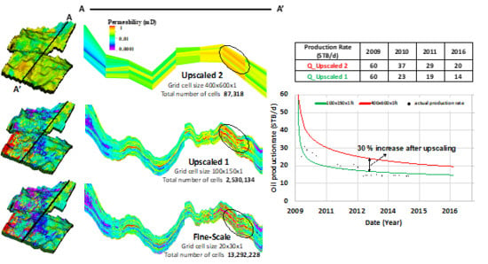
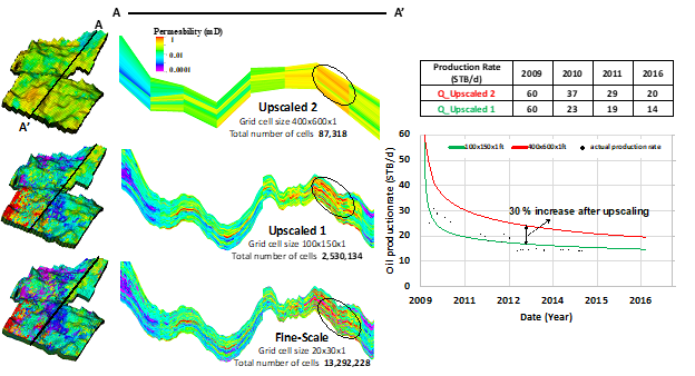
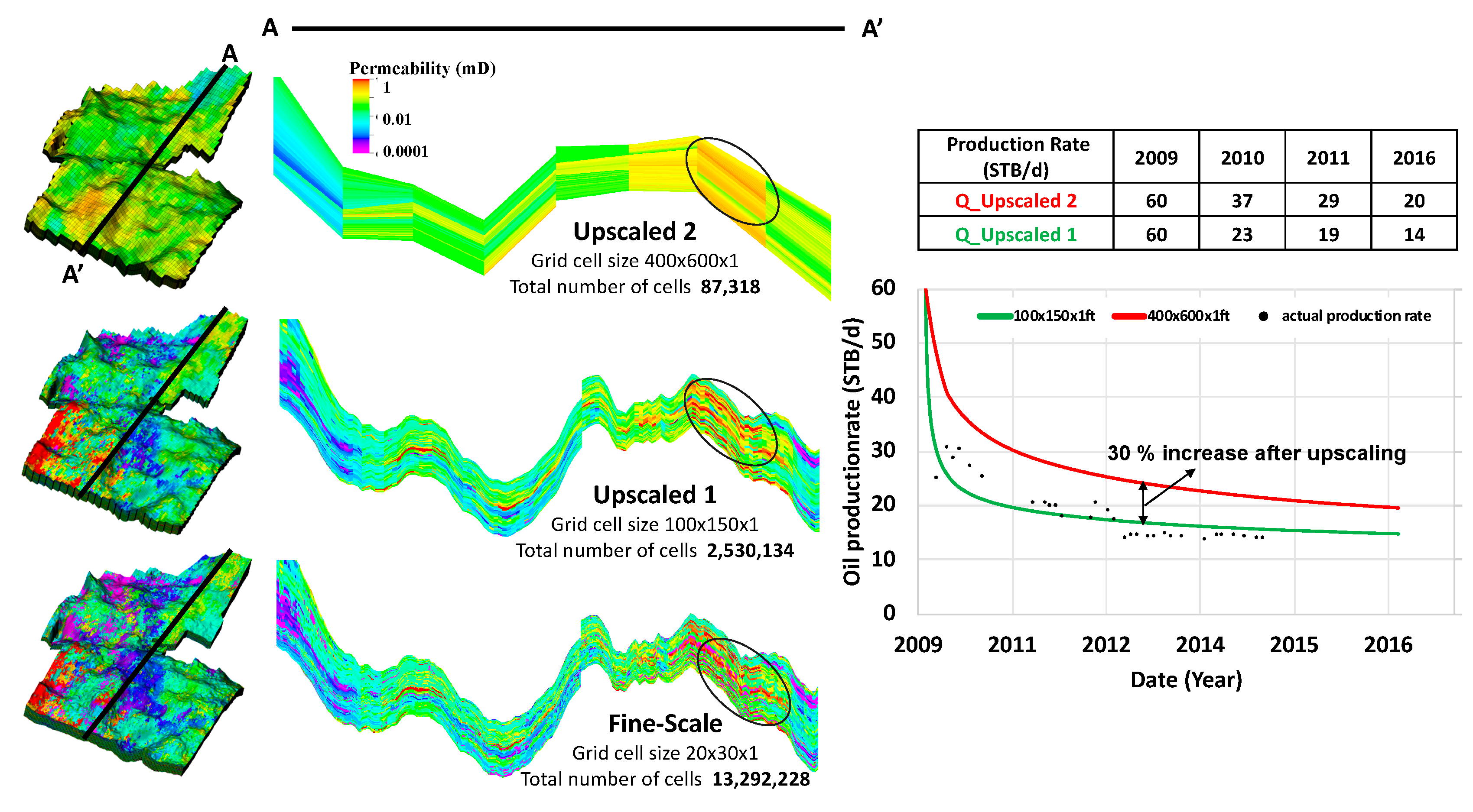
Figure 1.
Illustrations of permeability upscaling processes that lead to loss of the detailed heterogeneities in the geologic model that directly affects the accuracy of production profile. The fine scale permeability model, which consists of more than 13 million cells, has cell sizes of 20 ft in X-direction, 30 ft in Y-direction, and 1 ft in vertical (Z) direction. This model was upscaled by enlarging the grid size (reducing the number of cells to 2,530,134) and averaging the permeabilities. Similar process was repeated for the excessively upscaled model resulting in only 87,000 cells. Note the permeability heterogeneities along A-A’ section are not the same, especially in the black oval shape. The right figure shows the change in production rate over time for the two upscaled models. The fine scale model could not be run on our computers as handling 13 million cells is beyond their capacity. Notice the 30% increase in production rate after upscaling (Upscaled 1 to Upscaled 2).
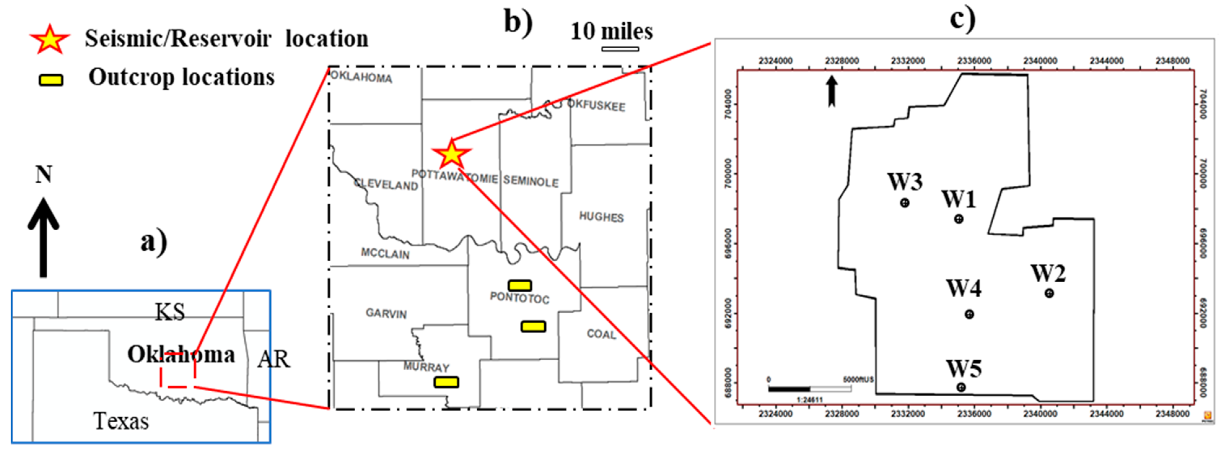
Figure 2.
Locations of the studied areas. (a) Oklahoma map with adjacent states. (b) Data locations in Pottawatomie, Pontotoc, and Murray Counties. Location of three-dimensional (3D) seismic, subsurface log and cores data in Pottawatomie County is indicated by the star. Yellow bars indicate outcrops in Pontotoc and Murray Counties. (c) Limits of the Pottawatomie County survey showing subsurface well locations.
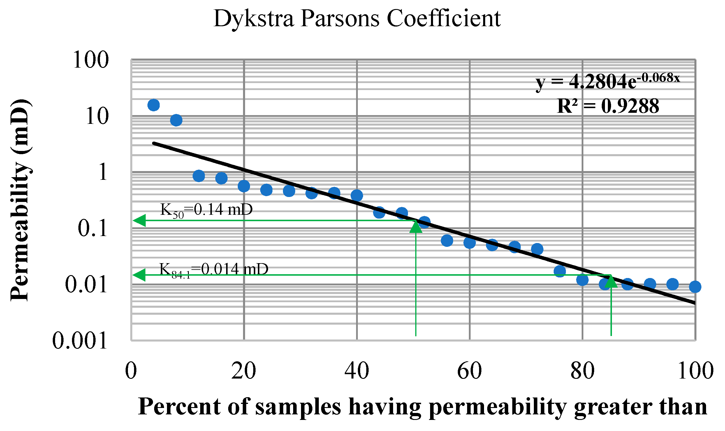
Figure 3.
Dykstra Parsons analysis for core permeability measured in this study.
Figure 3.
Dykstra Parsons analysis for core permeability measured in this study.
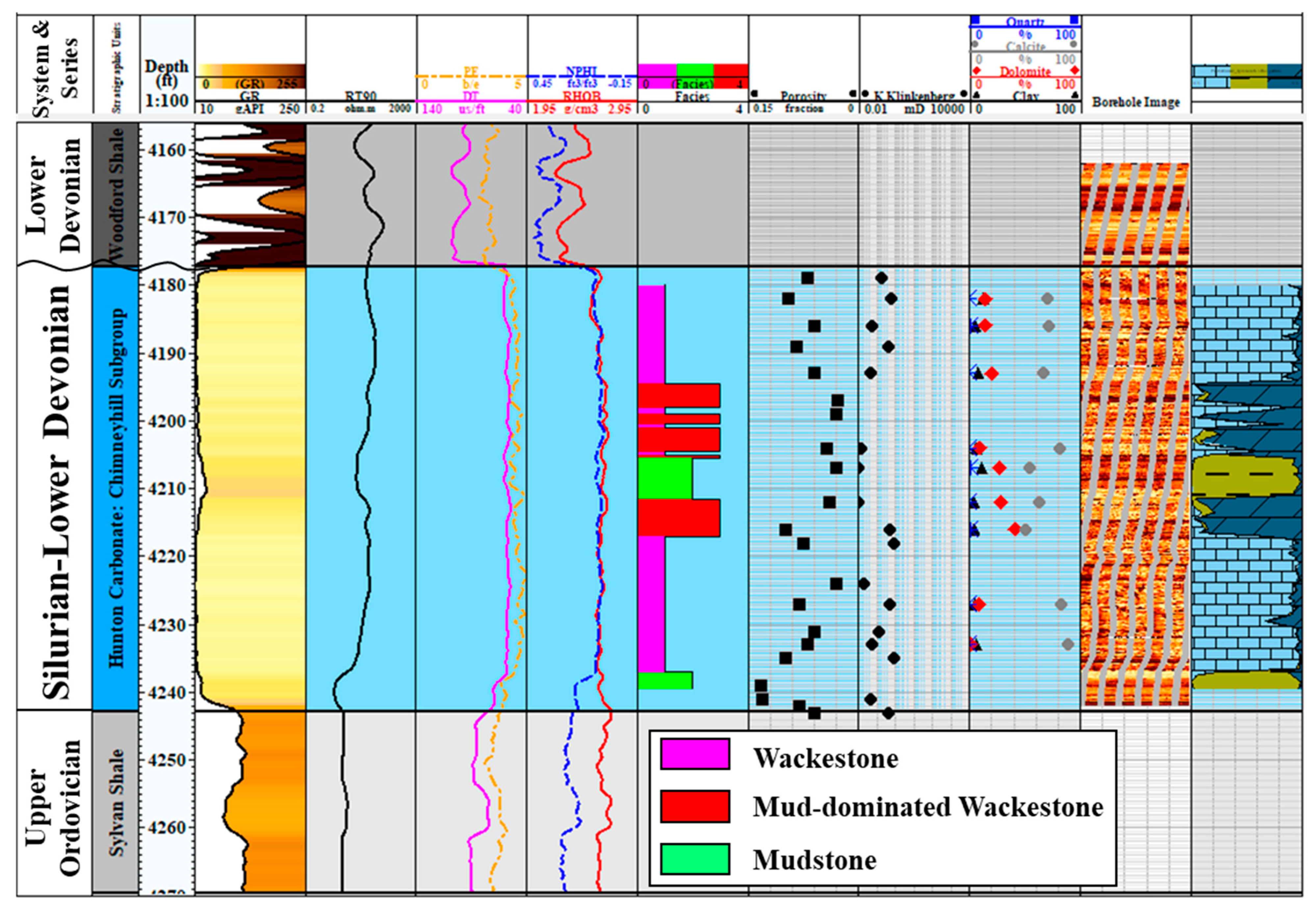
Figure 4.
Stratigraphic column of the Chimneyhill subgroup of the Hunton Group carbonate in the study area (Pottawatomie County, Oklahoma) from a subsurface well. Tracks from left to right are: geologic time, stratigraphic units (Viola carbonate, Sylvan shale, Hunton Group carbonate, and Woodford shale), true vertical depth (ft), gamma ray, deep resistivity (RT90), photoelectric (PE), and sonic (DT) logs, neutron porosity (NPHI) and bulk density (RHOB), electrofacies, core porosity, core permeability, core mineralogy, borehole image, and lithology.
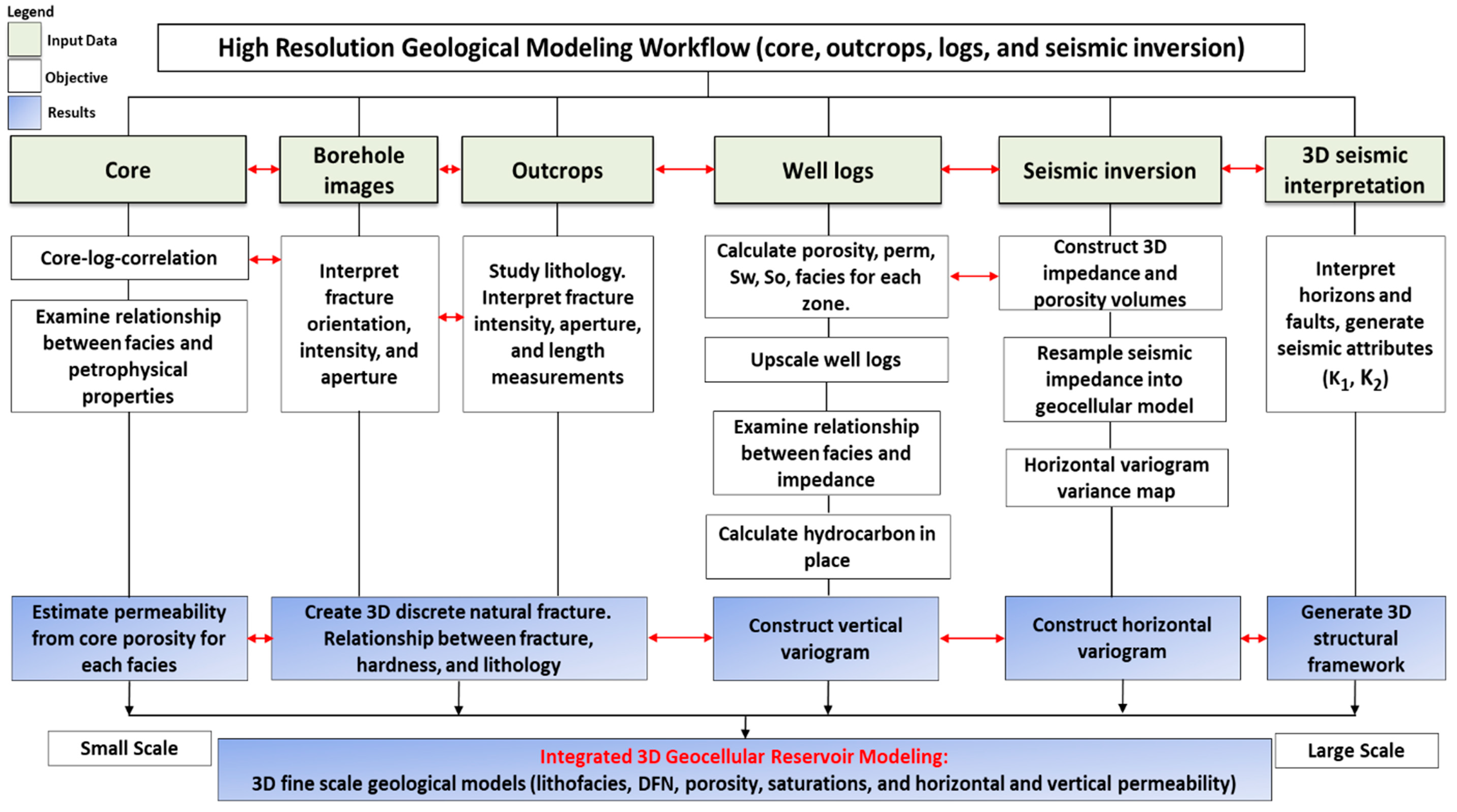
Figure 5.
Methodology depicting the integration of various sources of data for building the static reservoir model.
Figure 5.
Methodology depicting the integration of various sources of data for building the static reservoir model.
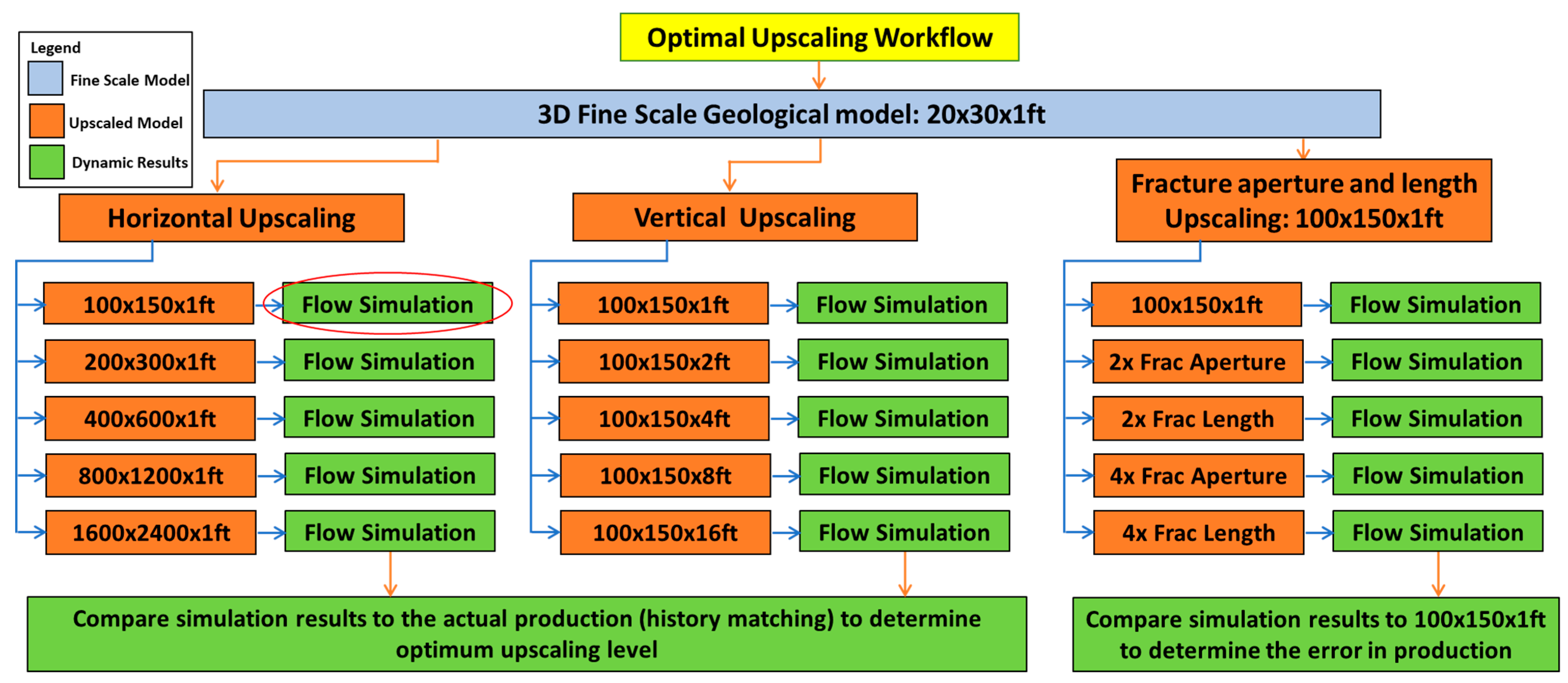
Figure 6.
Workflow depicting history match. The reference fine grid has cells that measure Δx = 20 ft, Δy = 30 ft, and Δz = 1 ft. Flow was simulated for the coarser horizontally and vertically upscaled models, as well as for the models with upscaled fracture lengths and apertures.
Figure 6.
Workflow depicting history match. The reference fine grid has cells that measure Δx = 20 ft, Δy = 30 ft, and Δz = 1 ft. Flow was simulated for the coarser horizontally and vertically upscaled models, as well as for the models with upscaled fracture lengths and apertures.
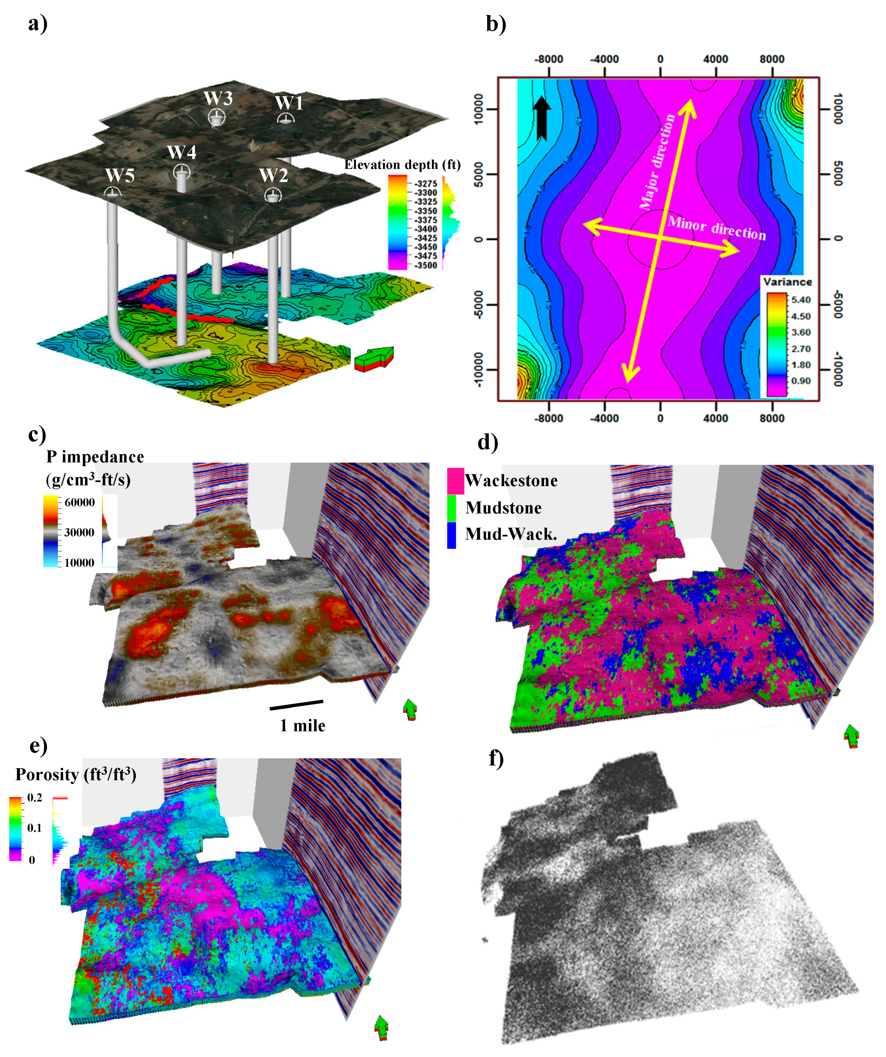
Figure 7.
Results of fine scale model. (a) Wells showing four vertical and one horizontal well trajectories. (b) Major and minor variogram directions derived from impedance maps of seismic inversion (major direction: N15E, major range: 18,840 ft, minor direction: S75E, minor range: 15,800 ft). (c) Impedance map from inversion. (d) Lithology derived from seismic impedance map. (e) Porosity maps from the inversion-derived variogram. (f) Discrete fracture network (DFN) map of the North East-South West (NE-SW) fracture set. All other sets have similar spatial relative density variation.
Figure 8.
Static heterogeneous models upscaled to 100 × 150 × 1 ft grid cell size: (a) porosity, (b) water saturation, (c) horizontal permeability, and (d) vertical permeability. Vertical exaggeration is 20 times.
Figure 8.
Static heterogeneous models upscaled to 100 × 150 × 1 ft grid cell size: (a) porosity, (b) water saturation, (c) horizontal permeability, and (d) vertical permeability. Vertical exaggeration is 20 times.
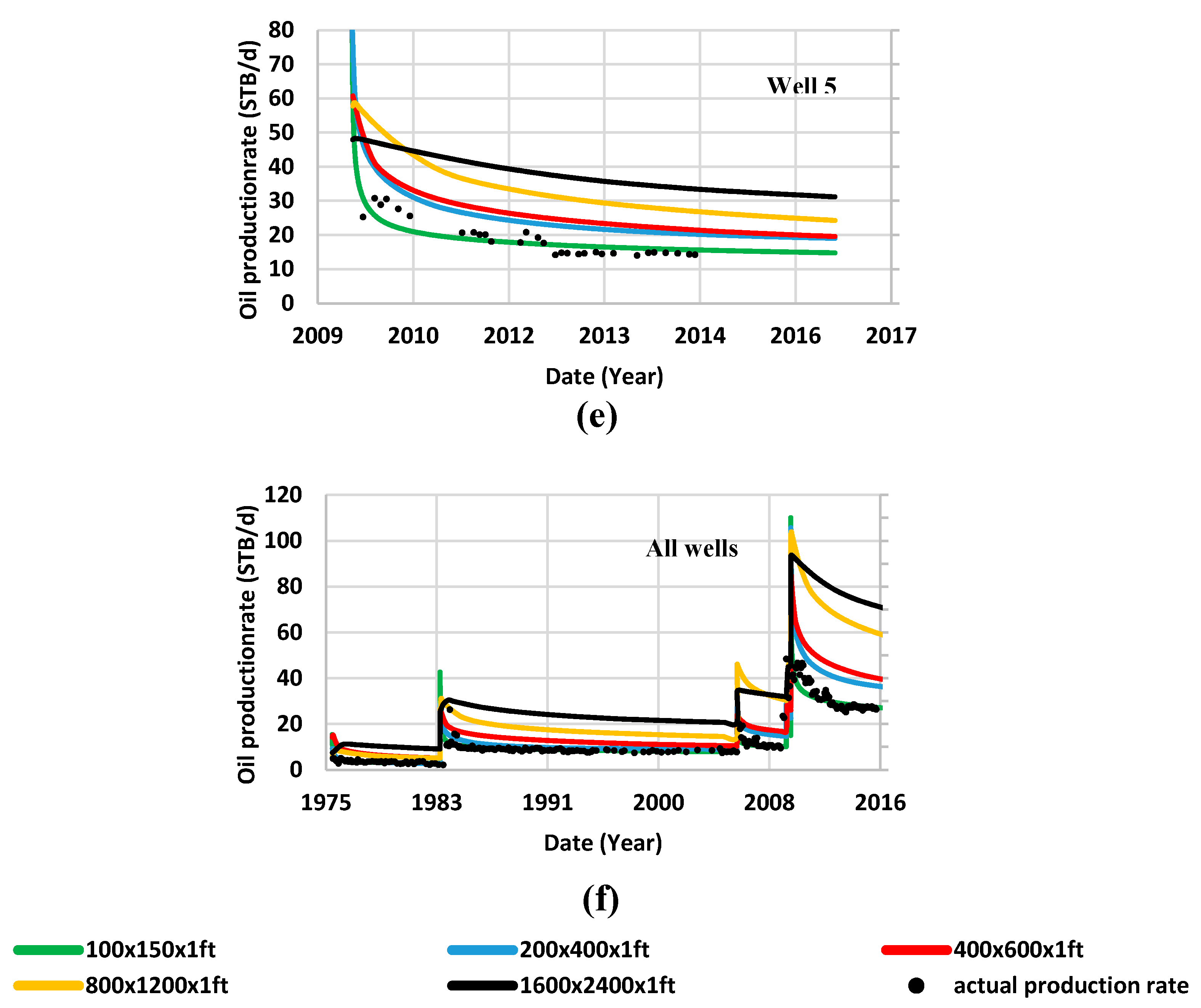
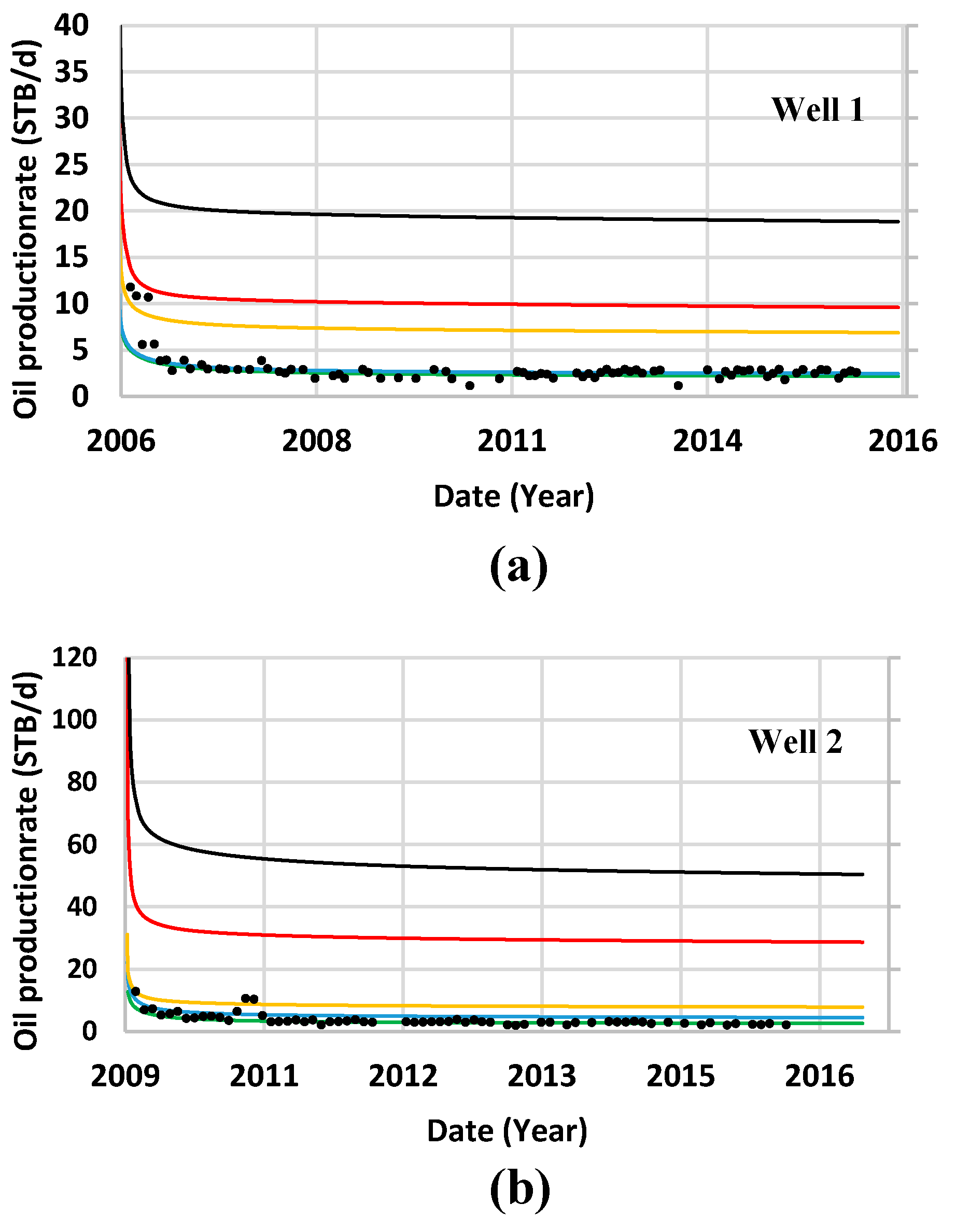
Figure 9.
Effect of horizontal upscaling on production. (a–e) Rate production for wells 1–5 respectively. (f) Production rates for all wells. Dots: actual production rates; Production rates for different grid cell sizes—green curves: 100 × 150 × 1 (history match); blue curves: 200 × 300 × 1; red curve: 400 × 600 × 1; orange curves: 800 × 1200 × 1; black curves: 1600 × 2400 × 1.
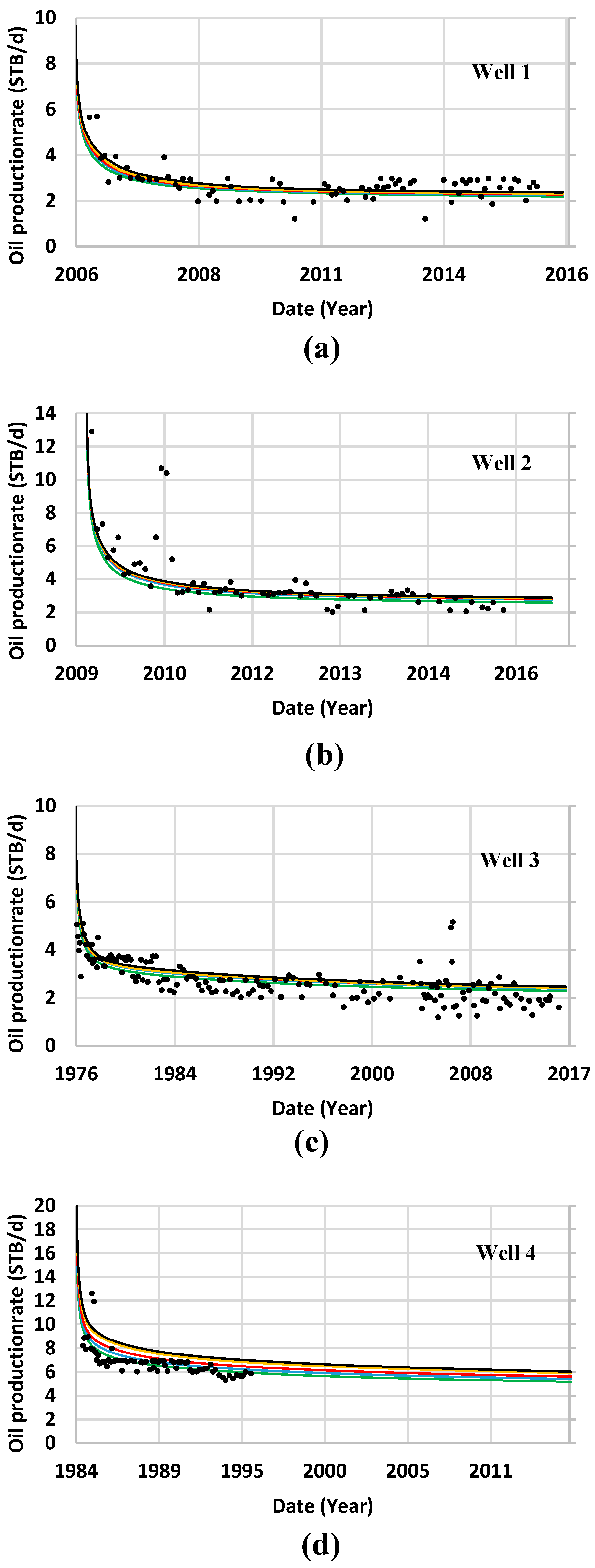
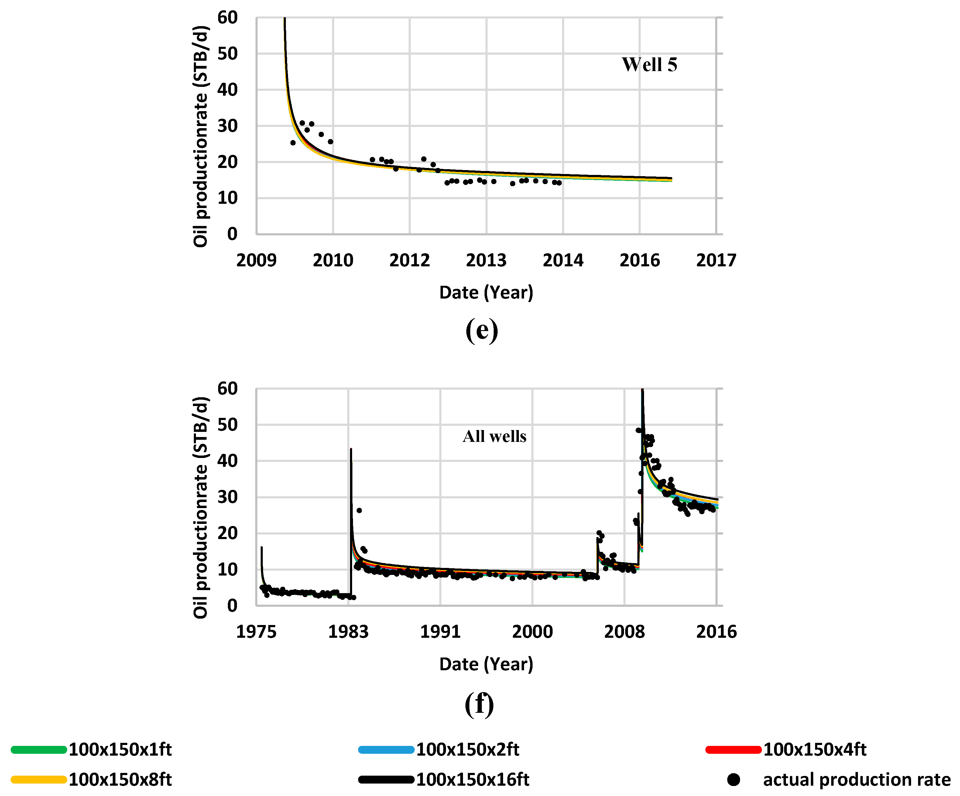
Figure 10.
Effect of vertical upscaling on production rate. (a–e) Production rate for individual wells. (f) Sum of production rates for all wells (field production). The difference in the field production dates is due to different start time of production for these five wells. Dots: actual production rates; production rates for different grid cell sizes—green curves: 100 × 150 × 1 (approximate history match); blue curves: 100 × 150 × 2; red curve: 100 × 150 × 4; orange curves: 100 × 150 × 8; black curves: 100 × 150 × 16 of cumulative production for individual wells.
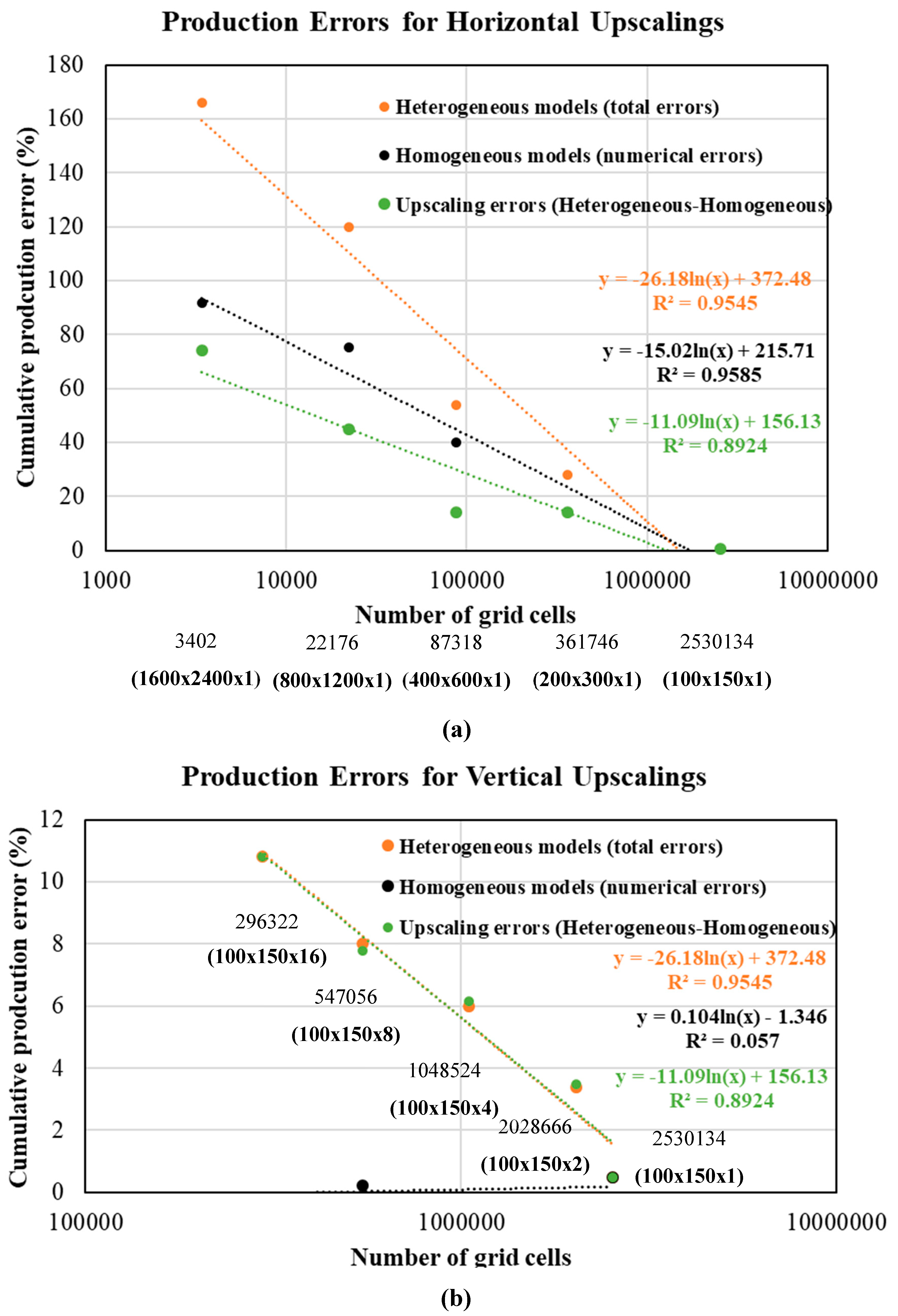
Figure 11.
Comparison between vertical and horizontal upscaling production error. Total errors that are associated with numerical errors and rock heterogeneity due to upscaling (orange), numerical (uncertainty) error resulting from the truncation computational errors (black), and upscaling errors (rock heterogeneity) resulting from changes in grid cell sizes (green). Some orange points are overlapping black points in the upper plot (
a) and black points are overlapping each other on the lower plot (
b). a) Semilog plot depicting logarithmic best-fit equations (inversely proportional) for the three horizontal upscaling curves (orange, black, and green). Note numerical production errors due to the computational truncation errors (black) are higher than the production errors due to the upscaling of geologic heterogeneity (green) for grid cell sizes. The exact error values for the horizontal upscaling are found in the last columns ("all wells combined") in
Table 3,
Table 4, and
Table 5. b) Semilog plot depicting logarithmic best-fit equations (inversely proportional) for the total errors and numerical errors vertical upscaling. Note numerical errors with the vertical upscaling is very low (black). Note much lower numerical errors with vertical upscaling (black) and higher errors with horizontal upscaling (black). The exact error values for the vertical upscaling are found in the last columns ("all wells combined") in
Table 6,
Table 7, and
Table 8.

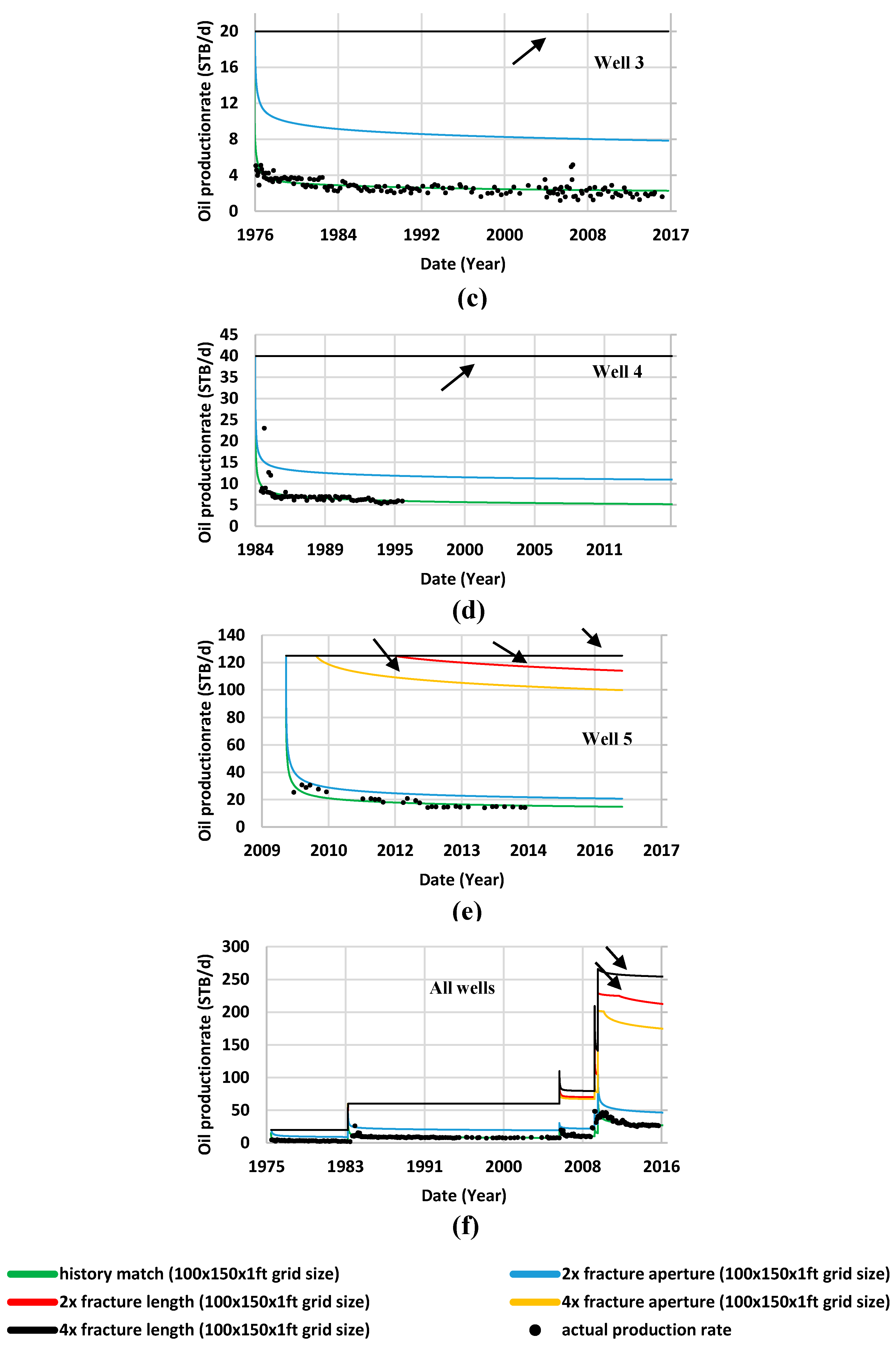
Figure 12.
Effect of fracture aperture and length on production rate showing history match curves, 2x, and 4x fracture length and aperture. Arrows indicate curves, which may be considered as incorrect due to constant production rates over long periods because model boundaries were probably reached due to high connectivity. (a) and (b) show all curves correctly. (c), (d), and (e) show history match, 2x length, and 2x apertures correctly but not 4x. Dots: actual production rates, Solid green: history match, Solid red: 2x fracture length, Broken red: 4x fracture length; Solid blue: 2x fracture aperture, Broken blue: 4x fracture aperture.
Figure 13.
Time required for flow-simulation completion. (a) Log-log plot depicting simulation time required using a different number of grid cells (or grid cell size) while applying different numbers of processes: a single (blue), five (orange), ten (red), twenty (black) processes. All curves were best fit by a power law. (b) Plot (both x and y-axes are linear) depicting simulation time using different number of processes (curves depicting single grid cell sizes) while using various grid cell sizes: 100 × 150 × 1 (green), 200 × 300 × 1 (blue), 400 × 600 × 1 (red), and 800 × 1200 × 1 (orange). All curves were best fit by negative power law equations.
Table 1.
Reservoir simulation parameters for the homogenous models used in all vertical and horizontal upscaling and production simulation cases. Where: Փ= porosity; Kv= matrix permeability in vertical direction; Sw: water saturation; KI, KJ, KK: fracture permeability in x, y, and z directions. Sigma factor: link between the matrix and fracture properties that describes fluid flow between the matrix and the dual-porosity/permeability model in a porous medium. If Sigma factor = 0, no communication between the matrix and natural fractures occurs.
| Matrix Parameters | Natural Fracture Parameters |
|---|
| Parameters | Average Values | Units | Parameters | Average Values | Units |
|---|
| Փ | 0.07 | Fraction | Փ | 0.00009 | Fraction |
| K in X direction | 0.131 | mD | KI | 1 | mD |
| K in Y direction | 0.131 | mD | KJ | 1 | mD |
| KV | 0.0001 | mD | KK | 1 | mD |
| Sw | 5 | % | Sigma factor | 7.6 | dimensionless |
Table 2.
Reservoir simulation parameters and well data constraints. These data are kept the same for all upscaling simulation cases. STB/d: Stock Tank Barrels per day; API: American Petroleum Institute.
Table 2.
Reservoir simulation parameters and well data constraints. These data are kept the same for all upscaling simulation cases. STB/d: Stock Tank Barrels per day; API: American Petroleum Institute.
| Well Rate and Pressure Constraints | Fluid Model Parameters |
|---|
| Well No | Oil rate (STB/d ) | Phases | Gas, Oil, Water |
|---|
| Well 1 | 50 | Min pressure | 300 psi |
| Well 2 | 130 | Max pressure | 2000 psi |
| Well 3 | 20 | Reference pressure | 1860 psi |
| Well 4 | 40 | Temp. | 170.33 oF |
| Well 5 | 125 | Gas Sp.gr | 0.815 |
| Simulation period: 1976-January to 2016-December | Oil gravity | 45 API |
| Bubble point pressure | 1860 psi |
| Water salinity | 30,000 ppm |
Table 3.
Cumulative production comparisons in horizontal upscaling cases for the heterogeneous models. Well by well actual cumulative production, history-matched (100 × 150 × 1 grid) cumulative production, and comparisons of larger grid cell sizes with history-matched cumulative production are shown. Errors in the history match column are with respect to the actual cumulative production and those in remaining columns are with respect to the history-matched production.
| | Actual Cumulative Production (STB) | 100 × 150 × 1 (History Match) Cumulative production error | 200 × 300 × 1 Cumulative Production Error | 400 × 600 × 1 Cumulative Production Error | 800 × 1200 × 1 Cumulative Production Error | 1600 × 2400 × 1 Cumulative Production Error |
|---|
| Well 1 | 10,170 | 9626 (–5%) | +131% | +155% | +345% | +537% |
| Well 2 | 10,217 | 7542 (–26%) | +62.6% | +99% | +261% | +285% |
| Well 3 | 37,398 | 39,634 (6%) | –4% | +71% | +72% | +189% |
| Well 4 | 27,348 @ 1995 | 29,333 (7%) | +22% | +29% | +100% | +153% |
| Well 5 | 37,956 @ 2014 | 34,254 (–10%) | +36% | +44% | +80% | +106% |
| All wells combined | 175,064 | 170,015 (0.5%) | +28% | +54% | +120% | +166% |
Table 4.
Cumulative production comparisons in horizontal upscaling cases for the homogenous models. Well by well actual cumulative production and comparisons of larger grid cell sizes with 100 × 150 × 1 ft history matched grid cell size are shown.
Table 4.
Cumulative production comparisons in horizontal upscaling cases for the homogenous models. Well by well actual cumulative production and comparisons of larger grid cell sizes with 100 × 150 × 1 ft history matched grid cell size are shown.
| | 100 × 150 × 1 Cumulative Production Error | 200 × 300 × 1 Cumulative Production Error | 400 × 600 × 1 Cumulative Production Error | 800 × 1200 × 1 Cumulative Production Error | 1600 × 2400 × 1 Cumulative Production Error |
|---|
| Well 1 | 107.99% | 16.57% | 50.48% | 85.95% | 123.84% |
| Well 2 | 69.55% | 19.12% | 54.95% | 91.25% | 121.43% |
| Well 3 | 54.01% | 11.91% | 32.00% | 67.21% | 92.54% |
| Well 4 | 131.78% | 12.78% | 35.50% | 66.05% | 72.97% |
| Well 5 | –36.87% | 16.56% | 50.30% | 79.46% | 108.21% |
| All wells combined | 4.77% | 14.02% | 39.90% | 75.22% | 91.78% |
Table 5.
Cumulative production comparisons in horizontal upscaling cases after subtracting the numerical errors in
Table 4 from total errors in
Table 3 for 200 × 300 × 1, 400 × 600 × 1, 800 × 1200 × 1, and 1600 × 2400 × 1 cell sizes.
Table 5.
Cumulative production comparisons in horizontal upscaling cases after subtracting the numerical errors in
Table 4 from total errors in
Table 3 for 200 × 300 × 1, 400 × 600 × 1, 800 × 1200 × 1, and 1600 × 2400 × 1 cell sizes.
| | Actual Cumulative Production (STB) | 100 × 150 × 1 (History Match) Cumulative production error | 200 × 300 × 1 Cumulative Production Error | 400 × 600 × 1 Cumulative Production Error | 800 × 1200 × 1 Cumulative Production Error | 1600 × 2400 × 1 Cumulative Production Error |
|---|
| Well 1 | 10,170 | 9626 (–5%) | 114.43% | 104.52% | 259.05% | 413.16% |
| Well 2 | 10,217 | 7542 (–26%) | 43.48% | 44.05% | 169.75% | 163.57% |
| Well 3 | 37,398 | 39,634 (6%) | –15.91% | 39.00% | 4.79% | 96.46% |
| Well 4 | 27,348 @1995 | 29,333 (7%) | 9.22% | –6.50% | 33.95% | 80.03% |
| Well 5 | 37,956 @ 2014 | 34,254 (–10%) | 19.44% | –6.30% | 0.54% | –2.21% |
| All wells combined | 175,064 | 170,015 (0.5%) | 13.98% | 14.10% | 44.78% | 74.22% |
Table 6.
Cumulative production comparisons in vertical upscaling cases for the heterogeneous models showing total (numerical uncertainty plus geologic heterogeneity). Well by well actual cumulative production, history match (100 × 150 × 1) cumulative production, and comparisons of larger grid cell size with history match cumulative production are shown. Errors in the history match column are with respect to the actual cumulative production and those in remaining columns are with respect to the history match (i.e., not actual production) case (100 × 150 × 1).
| | Actual Cumulative Production (STB) | 100 × 150 × 1 (History Match) Cumulative production error | 100 × 150 × 2 Cumulative Production Error | 100 × 150 × 4 Cumulative Production Error | 100 × 150 × 8 Cumulative Production Error | 100 × 150 × 16 Cumulative Production Error |
|---|
| Well 1 | 10,170 | 9626 (–5%) | +2.3% | +3.8% | +4.9% | +7.6% |
| Well 2 | 10,217 | 7542 (–26%) | +6.7% | +8.7% | +9.4% | +10.9% |
| Well 3 | 37,398 | 39,634 (6%) | +4.4% | +5.7% | +5.7% | +8.3% |
| Well 4 | 27,348 @ 1995 | 29,333 (7%) | +4.3% | +8.5% | +14.6% | +17.1% |
| Well 5 | 37,956 @ 2014 | 34,254 (–10%) | +0.5% | +2.6% | +0.18% | +3.6% |
| All wells combined | 175,064 | 170,015 (0.5%) | +3.4% | +6.0% | +8.0% | +10.8% |
Table 7.
Cumulative production comparisons in vertical upscaling cases for the homogenous models showing errors due to numerical uncertainty. Well by well actual cumulative production and comparisons of larger grid cell sizes with (100 × 150 × 1 grid) cumulative production are shown.
Table 7.
Cumulative production comparisons in vertical upscaling cases for the homogenous models showing errors due to numerical uncertainty. Well by well actual cumulative production and comparisons of larger grid cell sizes with (100 × 150 × 1 grid) cumulative production are shown.
| | 100 × 150 × 1 Cumulative Production Error | 100 × 150 × 2 Cumulative Production Error | 100 × 150 × 4 Cumulative Production Error | 100 × 150 × 8 Cumulative Production Error |
|---|
| Well 1 | 108.02% | 0.00% | –0.07% | 0.18% |
| Well 2 | 69.55% | 0.09% | 0.25% | 0.59% |
| Well 3 | 54.01% | –0.05% | –0.09% | 0.12% |
| Well 4 | 131.78% | 0.01% | 0.27% | 0.86% |
| Well 5 | –36.87% | –0.58% | –1.96% | –1.59% |
| All wells combined | 4.77% | –0.07% | –0.17% | 0.21% |
Table 8.
Cumulative production comparisons in vertical upscaling cases after subtracting the numerical errors in
Table 7 from total errors in
Table 6 for 100 × 150 × 2, 100 × 150 × 4, 100 × 150 × 8, and 100 × 150 × 16 cell sizes.
Table 8.
Cumulative production comparisons in vertical upscaling cases after subtracting the numerical errors in
Table 7 from total errors in
Table 6 for 100 × 150 × 2, 100 × 150 × 4, 100 × 150 × 8, and 100 × 150 × 16 cell sizes.
| | Actual Cumulative Production (STB) | 100 × 150 × 1 (History Match) Cumulative production error | 100 × 150 × 2 Cumulative Production Error | 100 × 150 × 4 Cumulative Production Error | 100 × 150 × 8 Cumulative Production Error | 100 × 150 × 16 Cumulative Production Error |
|---|
| Well 1 | 10,170 | 9626 (–5%) | 2.30% | 3.87% | 4.72% | 7.60% |
| Well 2 | 10,217 | 7542 (–26%) | 6.61% | 8.45% | 8.81% | 10.90% |
| Well 3 | 37,398 | 39,634 (6%) | 4.45% | 5.79% | 5.58% | 8.30% |
| Well 4 | 27,348 @ 1995 | 29,333 (7%) | 4.29% | 8.23% | 13.74% | 17.10% |
| Well 5 | 37,956 @ 2014 | 34,254 (–10%) | 1.08% | 4.56% | 1.77% | 3.60% |
| All wells combined | 175,064 | 170,015 (0.5%) | 3.47% | 6.17% | 7.79% | 10.80% |
Table 9.
Cumulative production comparisons for history match, 2x, and 4x fracture aperture and fracture lengths. Errors in the history match column are with respect to the actual cumulative production and those in the remaining columns are with respect to the history match (i.e., not actual) production case (100 × 150 × 1).
| | Actual Cumulative Production (STB) | 100 × 150 × 1 (history match) cumulative production error | 2X Fracture Aperture Cumulative Production Error | 4X Fracture Aperture Cumulative Production Error | 2X Fracture Length Cumulative Production Error | 4X Fracture Length Cumulative Production Error |
|---|
| Well 1 | 10,170 | 9626 (–5%) | +11% | +190% | +301% | +673% |
| Well 2 | 10,217 | 7542 (–26%) | +63% | +169% | +861% | +1596% |
| Well 3 | 37,398 | 39,634 (6%) | +224% | 642% | +642% | 642% |
| Well 4 | 27,348 @ 1995 | 29,333 (7%) | +86% | 470% | +470% | 470% |
| Well 5 | 37,956 @ 2014 | 34,254 (–10%) | +37% | 480% | +539% | 555% |


