1. Introduction
A small step towards the validation of numerical solvers able to accurately replicate the behavior of supercritical fluid flows is to understand how current RANS (Reynolds Averaged Navier Stokes) turbulence models, calibrated and tested for subcritical conditions, behave in the supercritical regime. The use of accurate thermodynamic formulations capable of capturing the singular behavior of supercritical fluids allows for the efficiency and accuracy of each turbulence model to be tested, and their structure or the presence of specific terms linked to the characteristics of the final results.
A supercritical fluid is characterized by pressure and temperature above the fluid’s critical values. In fuel injection phenomena, specifically in combustion chambers, both fuels and oxidizers’ operating conditions can exceed their critical point as a means to increase the engine’s efficiency [
1,
2,
3]. At an arbitrary constant temperature, a gas can be converted to a liquid by increasing the pressure. As temperature increases, so does the kinetic energy of the molecules, requiring a higher pressure to bring the gas to a liquid. The critical temperature,
, marks the point after which a transition to the liquid phase is no longer possible, no matter the applied pressure. The vapor pressure at the critical temperature is then defined as the critical pressure,
. The critical point then marks the end of the vapor pressure line, where both temperature and pressure reach their critical values.
Since vaporization no longer occurs, a more suitable terminology is needed. Several authors, including [
4], propose the use of “emission rate“ and “emission constant“ to describe mixing under supercritical conditions.
As the temperature increases even further, the liquid-like supercritical oxidizer crosses the pseudocritical line and transitions to a gas-like fluid. This transition from a liquid-like to a gas-like state could be compared to a subcritical boiling, the main difference being that the isothermal vaporization typical of subcritical fluids is replaced by a continuous non-equilibrium process that takes place over a finite temperature range (
Figure 1). As this happens, the specific heat capacity goes through a maximum and tends to infinity when approaching the critical point, as shown in
Figure 2. Similarly to [
5], we refer to this transition phenomenon as pseudo-boiling and the maxima of the specific heat capacity as pseudo-boiling of pseudocritical line. It represents then a continuation of the saturation line well into the supercritical regime.
The two parameters
and
can therefore be used to identify pseudo-boiling temperatures for different pressure values as shown in
Figure 2. For nitrogen, it is visible that as the pressure approximates the critical value of 3.39 MPa, the peak in specific heat becomes more noticeable along with the slope of
.
It is well known that in a subcritical injection, surface instabilities are responsible for jet atomization, small discrete ligaments begin to break up, and droplets are ejected from the jet core [
6]. In a supercritical injection, however, the breakup mechanics are entirely different. [
7] describes one of the main characteristics of supercritical fluids as the impossibility of a two-phase flow. Similar effects are reported by [
5], where the surface tension is measured for oxygen from subcritical temperatures, with higher values, up to the critical temperature, for which it completely vanishes. Several other authors describe this different breakup mechanism where the drops and ligaments are no longer detected, and no distinct surface interface can be determined. [
7] notes that this disintegration mechanism more closely resembles turbulent and diffusive mixing than the traditional jet disintegration and [
8] describes a thermal-breakup mechanism where the limit of the jet core is defined by the transition of the fluid across the pseudocritical line.
In the end, both the thermodynamic behavior and the breakup mechanisms have a direct effect on the jet structure. As the liquid-like nitrogen is injected into the chamber, its temperature increases as it begins to mix with a warmer gas, such as nitrogen. The structure of the flow changes and it can be divided into three characteristic regions: potential core, transition, and fully developed region. [
9] defines the length of the potential core as the distance at which the centreline density remains relatively constant and [
8] compiles and compares four different equations attempting to predict this length that is either based on the ratio between the densities of the liquid and gas-like fluids or are given a constant value for any specific test geometry. In the self-similar region, the absolute value of flow variables can still change, but their radial profiles are no longer a function of axial direction. In between these two regions lies the transition zone, where the turbulent and diffuse mixing is most relevant. As instabilities begin to appear, dense pockets of liquid-like nitrogen are separated from the jet core, causing an increase in density fluctuations [
10,
11]. As a result, the density sharply decreases, and the energy dissipation is significant. In experimental studies, this structure is visible through the axial and radial density distributions and also through the jet spreading angle.
Turbulence is regarded as the last unsolved problem of classical physics. The presence of advective terms in the governing equations leads to their admittance of a chaotic solution after a critical Reynolds number. Modeling is then performed resorting to techniques such as RANS (Reynolds Averaged Navier Stokes), LES (Large Eddy Simulation), or DNS (Direct Numerical Simulation). However, when discussing supercritical fluid flows, the fact that no turbulence models developed explicitly for flows at these conditions exist, is an added factor of uncertainty. Throughout the years, these techniques have been used in the modeling of supercritical fluid flows with various degrees of success.
In a series of studies by the same authors, [
12,
13,
14], a Large Eddy Simulation solver is used for the computation of nitrogen injection. In this sense, [
15] also perform LES following a pressure-based solution approach in which the PISO - Pressure-Implicit with Splitting of Operators algorithm for pressure-velocity coupling is employed. The authors conclude that further improvements are needed in the variables discretization so that the numerical diffusivity can be lowered.
The paths available in terms of discretization of the governing equations as well as in turbulence modeling are so diverse it justifies a study on how different approaches and modeling techniques affect the result. On this subject, [
16] performs a comparison between different RANS derivations of the
model and an LES computation. Cubic equations of state performance are compared and coupled with the compressible formulation for the conservation of mass and momentum. As for the temperature and transport properties, they are retrieved as a function of the mixture fraction.
In [
17], LES simulations are carried out, and a comparison is made between a density-based and a pressure-based solution. In the density-based solution, implicit LES combines turbulence modeling with the numerical discretization of the conservation equations, while in the pressure-based solution, an eddy viscosity approach is favored. The results comparison from the two solution approaches does not indicate a very substantial difference in the axial centerline distribution. Another LES pressure-based solution approach is proposed by [
18], using different sub-grid scale models. Also, on the subject of supercritical injection, [
19], conclude pressure-based solvers are strongly affected by the deviation of compressibility coefficients from the ideal gas behavior, and [
20] propose an extension of a double-flux model to real fluid equations of state, as a means to improve the capability of the numerical solver to cope with spurious pressure oscillations, especially close to the pseudocritical line.
In terms of Direct Numerical Simulation (DNS), the work of [
10] stands out, in which a lower inlet velocity is used, reducing the Reynolds number. A merged PISO/ SIMPLE algorithm allows for the study of entropy production rates, dominated by heat transfer [
21].
In high Reynolds numbers simulations, the choice then lies between RANS- and LES-based simulations. While RANS relies on the same turbulence model for the entire inertial scales, in LES, the larger inertial scales are solved, and an SGS (Sub-Grid Scale) model is used for the smaller scales. A filter is used to separate resolvable and Sub-Grid Scales. The importance of Sub-Grid Scale modeling in high-pressure LES computations is outlined by [
22]. Even though the potential of LES simulations is recognized, it has failed to outperform RANS-based solvers systematically. As a result, in the present work, a RANS-based numerical solver is used to compare the performance and accuracy of several turbulence models in the modeling of supercritical fluid flows. Specifically, the validation of a numerical setup replicating combustion chamber conditions can be seen as a first step towards accurately and reliably simulating combustion phenomena inside a Liquid Rocket Engine combustion chamber, and a small step in this direction is to understand how current turbulence models behave under supercritical conditions and how their accuracy stands up against one another. The same issue was dealt with in a previous work [
23], through the reassessment of the concept of a variable turbulent Prandtl number, applied to the standard
turbulence model.
Interestingly enough, the comparison described can be linked to the general state of the space sector. The dawn of space exploration privatizing has lead to a boost and renewed interest in the modeling of vehicles used for such missions. As a consequence, an ever-increasing demand for economic sustainability has lead to the necessity of developing new solutions for space technology. As stated by by [
15], the new challenge is not the development of new technologies, but the improvement of already available concepts, with restricted budgets and shortened development cycles. In this sense, through the analysis of the RANS-based turbulence models here proposed an attempt is made to improve the knowledge regarding their behavior in the supercritical regime.
The remainder of this study is structured as follows: first, the experimental conditions necessary for validation purposes are shortly reviewed, and the initial and boundary conditions are established. The description of the governing equations in their Favre averaged formulation precedes the discussion about the adopted turbulence modeling; however, the models themselves are not detailed explained. Such an undertaking would not contribute to quality improvement of this manuscript, while would render it prohibitively extensive. A simple discussion of the models’ limitations and applicability is favored. The processes of density and transport properties determination are then discussed, as well as the discretization of the governing equations. The results are then critically analyzed, and the conclusions reiterated for future studies.
2. Initial and Boundary Conditions
The test cases from [
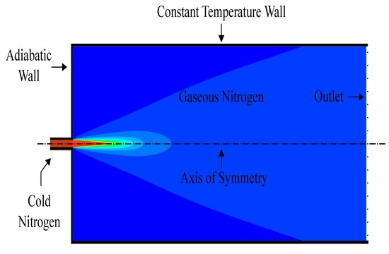
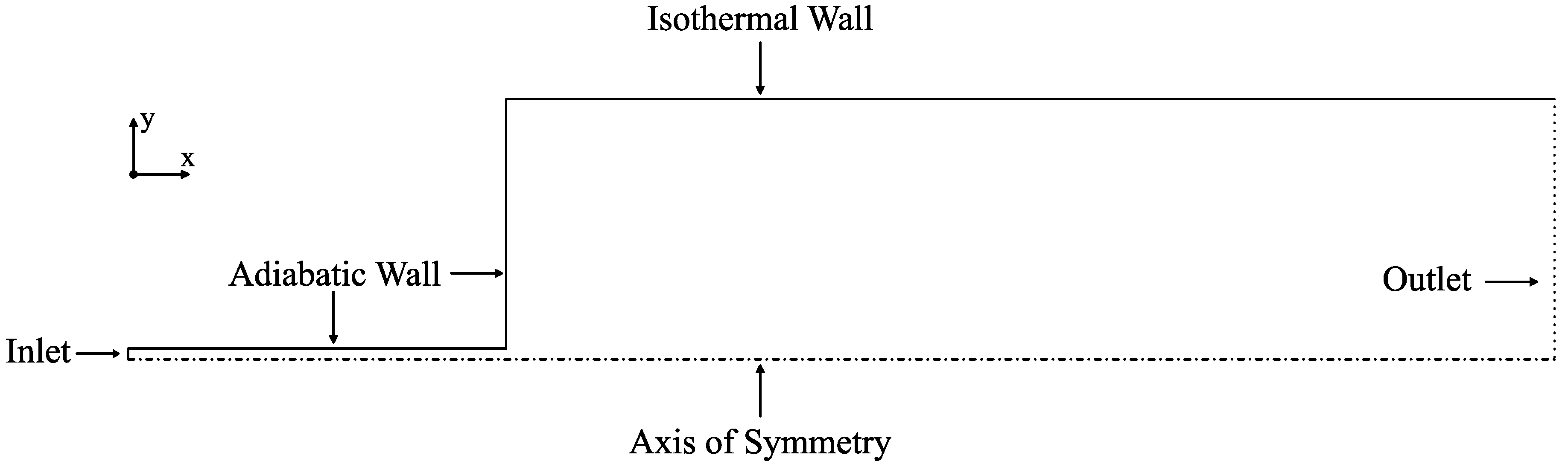
9] are the basis of comparison for this numerical study. In particular, case 3 and case 4 are investigated where cold nitrogen is injected into a chamber at ambient temperature with four windows for optical access.
The geometry corresponding to the experimental setup of [
9] is represented in
Figure 3. The diameter of the chamber and the injector are 122 mm and 2.2 mm, respectively, while measuring, in length, 250 mm and 90 mm. Liquid nitrogen is injected into a chamber filled with gaseous nitrogen according to the conditions indicated in
Table 1.The subscript 0 respects to injection conditions, with
∞ representing conditions in the combustion chamber.
The domain contains five different boundary conditions, also depicted in
Figure 3. A constant axial velocity profile is set at the inlet to
, and the radial velocity is set to zero. At the walls, a no-slip condition is applied where both the normal and tangential velocity components are set to zero.
A pressure outlet is defined with a gauge pressure of 0 MPa and where the pressure values at the outlet face are calculated by averaging the specified operating pressure of , with the internal pressure. Also, at the symmetry axis, the value of any specific property is equaled to that of the adjacent cell.
Finally, for the adiabatic walls of the injector and the faceplate, the heat flux from Equation (
1) is set to zero, but for the isothermal wall heat transfer is calculated through a Dirichlet boundary condition by setting a constant temperature at the wall of 297 K. In Equation (
1),
represents the fluid heat transfer coefficient,
the temperature at the wall and
is the local fluid temperature.
3. Governing Equations
To deal with the weakly incompressible but variable density conditions [
24], the standard time-averaging method is replaced by the Favre averaging procedure, and the system of equations is closed with different turbulence models, the main focus of this study. The performance of said models, designed and calibrated to run in subcritical conditions, is then studied and their validity for the supercritical regime is assessed.
The Favre averaging method introduces a density-weighted quantity (
) and a density-weighted fluctuation (
), as given by equation (
2) for an arbitrary scalar
.
is evaluated according to Equation (
3), being
the mean density.
The steady-state Favre averaged conservation equations for mass, momentum, and energy are reproduced here, following the integral formulation in Equations (
4) to (
6), respectively, where
represents density-weighted velocity components.
Mass can neither be created nor destroyed and as a result, there is no diffusive term in Equation (
4), only an advective one.
Momentum is a vectorial quantity meaning that its transport is defined by as many equations as the number of dimensions that are assumed. The momentum advective flux is then defined in Equation (
5) as
, while
represents the volume source term.
In Equation (
6), the advective term is represented by
, while the diffusive term is evaluated by Fourier’s law of conduction, through
and
is the Reynolds stress tensor.
The viscous stress tensor from Equations (
5) and (
6) is averaged according to Equation (
7), as a function of the molecular viscosiry where the mean strain-rate tensor,
, is given by Equation (
8) and
is the Kronecker delta function.
The Reynolds stress tensor of Equation (
5) holds correlations originated from the averaging process, given by Equation (
9).
Additional terms also appear in Equation (
6) such as the Favre-averaged total specific energy (
), enthalpy (
) and the turbulent heat flux (
), defined in Equations (
10), (
11) and (
12), respectively.
Lastly, the turbulence kinetic energy per unit volume,
k, is defined according to Equation (
13).
The double and triple correlations from Equations (
5) and (
6) are also a product of the averaging process which is too extensive to describe here. While a physical meaning can be attributed to some, it does not apply to others. The Reynolds stress tensor alone introduces three additional independent variables, meaning that the system is not yet closed. A transport equation for
can be provided, but the number of unknowns only increases, and the system remains open. Nevertheless, this is the essence of second-order turbulence models. For now, an approximation for
is needed.
4. Turbulence Models
The Boussinesq approximation can be used to define the Reynolds stress tensor and is the basis of turbulence modeling. This approximation relates
with the viscous stress tensor by introducing the concept of eddy or turbulent viscosity,
. It relates to the influence of molecular viscosity on the transport of momentum with the influence of turbulence viscosity on the transfer of momentum caused by turbulent fluctuations. As a result, Equation (
7) becomes:
While the terms for
are modeled through
, the trace of
is still precisely defined through the specific turbulent kinetic energy from Equation (
13) as:
With this relation, turbulence models can focus on calculating the eddy viscosity () and the turbulence kinetic energy (k).
The laminar and turbulent heat transport terms,
and
, are defined according to Fourier’s law, so that:
In Equation (
16), Pr
represents the turbulent Prandtl number, i.e.,
, where
is the eddy diffusivity of momentum and
the turbulent thermal diffusivity.
Finally, the molecular diffusion and the turbulent transport,
, are coupled together and modeled as shown in Equation (
17).
Turbulence models evaluate eddy viscosity in different ways but generally using the same properties, such as the turbulent kinetic energy, the turbulent dissipation rate, , and the specific dissipation rate, .
The mixing length hypothesis proposed by L. Prandtl provides an expression to define the turbulent viscosity based on the assumption that the x-momentum of fluid remains constant for a length of in the y-direction. is the mixing length that is characteristic of each flow geometry along with a characteristic velocity, that must be defined in advance. Ergo, zero equation models where the length and velocity scales are not defined through properties such as , or , are not independent of the case of study. One and two-equation models overcome this obstacle by introducing transport equations for history-dependent variables that can represent velocity and a length scale. Explicitly, the two-equation models studied in this work define the velocity scale through the turbulent kinetic energy to incorporate non-local and flow history effects in the turbulent viscosity. The underlying problem in RANS simulations results from the unavailability of velocity fluctuations, leading to the necessity of resorting to closure models. The chosen model involves, as do most of the choices made when attempting to numerically reproduce the behavior of supercritical fluid flows, a compromise between computational cost and accuracy. The current development of improved turbulence models faces the dilemma of conserving the low computational cost and high robustness of RANS approaches while incorporating as much physics as possible.
The Spalart–Allmaras model [
25] is a one-equation model in which a direct derivation of an equation for the transport of the modified eddy viscosity is performed. This does not happen on the
-based models [
26,
27,
28], where transport equations for both the turbulent kinetic energy (
) and its dissipation (
) are introduced. In the
-based models, the dissipation of turbulent kinetic energy is replaced by the specific dissipation rate, and as such, a variation of the model of [
29] is considered. The turbulent dissipation rate is replaced by the dissipation per unit time or specific dissipation rate defined as
.
In the standard model, additional terms related to low Reynolds numbers corrections and compressible effects are available for this model but are neglected for the current study. An attempt is made in reducing the round-jet anomaly by linking the dissipation of to the mean deformation of the flow. The predictions for k and outside of the shear layer remain on the most significant setbacks of this model, despite the introduction of a cross-diffusion term.
After the proposal of the Wilcox
model, [
30] developed the shear-stress transport (SST),
model, to retain the robust and accurate formulation of the Wilcox model inside the shear layer while taking advantage of the free-stream qualities of the
model in the far-field. The transport equation for
is converted into a similar formulation as that of
. This blending function is designed to be one in the viscous sublayer of the boundary layer and tend to zero in the log-law region (
).
All the models reasoned insofar are based on Boussinesq’s eddy viscosity concept. However, another one is considered, which does not have this concept as its underlying relationship. The Stress Baseline (BSL) model [
30] closes the system of governing equations with transport equations for
and
.
All these models are, however, subject to different levels of uncertainty, whose source identification remains a most challenging task due to the coupling between various phenomena and levels of uncertainty [
31]. Nevertheless, several studies were conducted on uncertainty quantification in several turbulence models, and even though the test subjects are not supercritical fluid flows, their conclusions are broad and extensive.
The application of sensitivity analysis (defined as the derivatives of the flow variables concerning the design parameters) by [
32] on a backward-facing step showed the calibration parameters
, and
in the
turbulence model, have the most pronounced effect on the turbulence model predictions. On the Spalart–Allmaras model, [
33] concludes the incomplete physical knowledge led to the use of dimensional analysis and a large amount of judgment to close or tune in model constants. Relations between coefficients need to be enforced to maintain the appropriate behavior of the Spalart–Allmaras model for canonical flows.
On the other hand, [
34] presents a novel methodology for improving eddy viscosity models in predicting wall-bounded turbulent flows with strong gradients in the thermophysical properties. Conventional turbulence models for solving the RANS equations do not correctly account for variations in transport properties, such as density and viscosity.
A methodology in which representative samples of motions and processes of all scales are solved and combined, while remaining computationally affordable, especially at large Reynolds numbers, effectively meaning the statistical resolution of all scales remains a somewhat distant goal.
Additionally, the turbulent kinetic energy, turbulent dissipation rate, and specific dissipation rate are based on the turbulent intensity,
I, and turbulent viscosity ratio,
:
In Equation (
18),
is specific to each of the turbulence models. In the Spalart–Allmaras model,
is taken directly from the turbulent viscosity ratio, and in the Stress-BSL model, the turbulent stresses are assumed to be zero, except for the trace of the tensor which is calculated as in Equation (
15). In all cases, the turbulence intensity is set to 5% at the inlet.
5. Equation of State and Transport Properties
In the supercritical regime, the ideal gas Equation of State (EoS) must be replaced by more accurate formulations. While multi-parameter EoS have high accuracy, they fall behind in terms of computational efficiency. To overcome this obstacle, in the present work, density values are loaded from a preexisting real gas library [
35], based on a reference equation of state for nitrogen [
36], allowing for increased accuracy at a reduced computational cost, since look-up tables are generated before the computations, effectively removing the need for thermophysical properties to be calculated in each iteration. The non-linearity of transport variables must also be accurately defined, and the equations proposed by [
37] are used.
Multiparameter equations of state can be created through polynomial and exponential expansions where the coefficients multiplied by each term are specific to each fluid. These coefficients must be fitted through the available experimental data for the conditions in which the EoS is to be valid. The 32-term modified Benedict-Webb-Rubin (MBWR) [
38] EoS achieves a relative density error smaller than 0.5% above and below the critical point, while [
39] proposes a 12-term EoS with available coefficients for a series of substances, nitrogen included, while [
40] provides a highly accurate 18-term EoS optimized directly for nitrogen.
The EoS presented by [
36] is based on the Helmholtz energy,
F, which is then normalized and set as a function of reduced temperature (
) and density (
):
The first right-hand-side term of equation (
19) refers to the ideal gas contribution to the Helmholtz energy while the second represents the residual Helmholtz energy corresponding to the intermolecular forces considered in a real gas formulation.
The ideal gas contribution is defined in Equation (
20), the residual addition is shown in Equation (
21) and the corresponding constants are listed in [
36]. Thermodynamic properties can then be calculated based on the derivatives of these two terms.
The coefficients specific to this EoS are obtained through data fitting methods based on experimental measurements from a series of authors and for a wide range of temperatures and pressures.
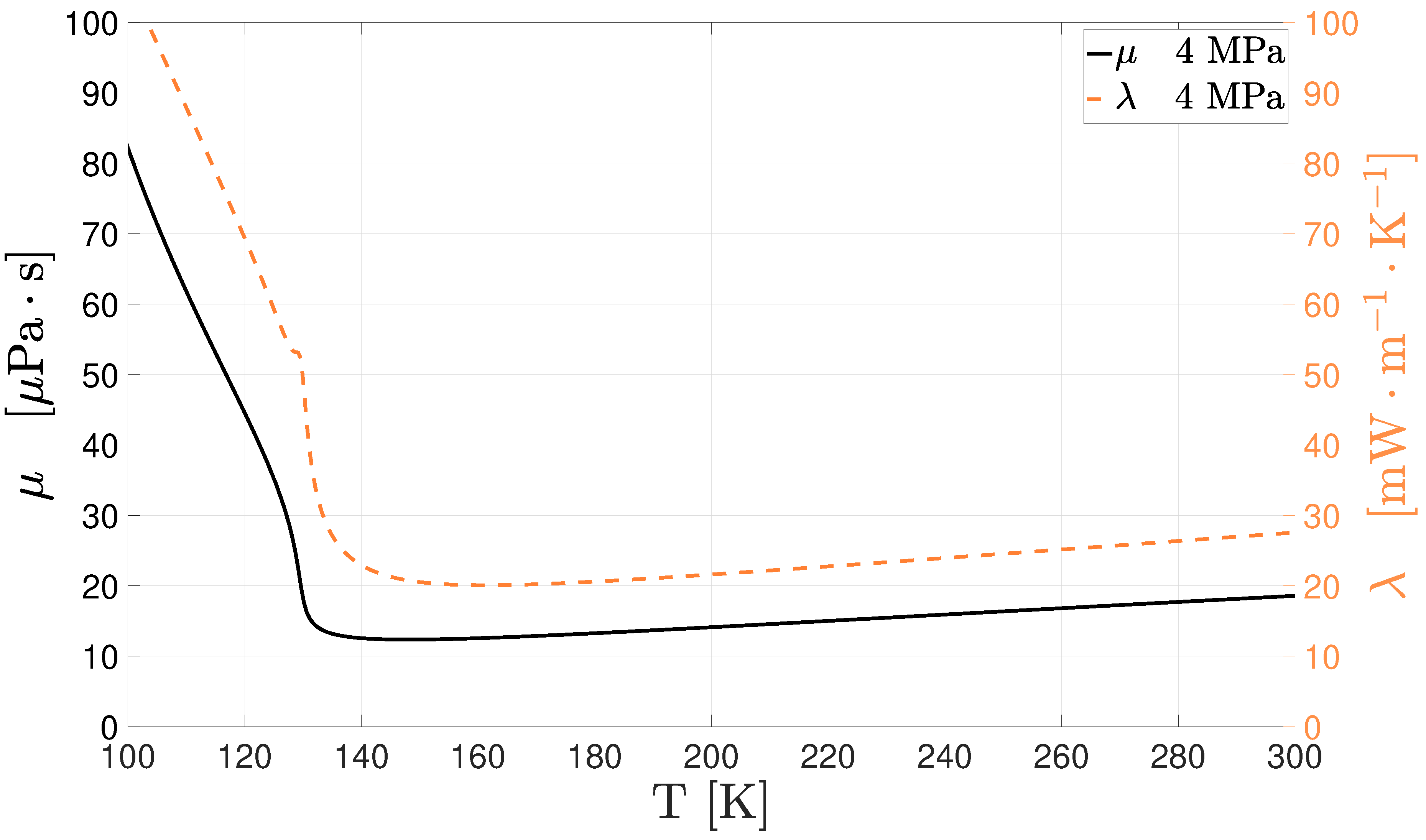
Transport properties have a direct impact on the governing equations. The substantial variation of transport properties as dynamic viscosity and thermal conductivity approaching and entering supercritical conditions is depicted for nitrogen in
Figure 4.
Following [
37], viscosity is expressed according to Equation (
22). Viscosity is evaluated from a dilute gas contribution,
(Equation (
23)) and a residual component,
, (Equation (
24)). The
represents the Lennard-Jones parameter and
the collision integral, while the remaining coefficients are tabulated in [
37].
In the same fashion, thermal conductivity is defined according to Equation (
25). The dilute and residual gas contributions are defined according to Equations (
26) and (
27), respectively.
A third component is needed for the evaluation of thermal conductivity in the critical region. Such contribution is defined in Equation (
28). The calculation of the
coefficients comes from the definition of specific heat at constant pressure and volume.
The use of real gas relationships for transport and thermodynamic properties allows the physical model to capture the weak compressibility effects when using an incompressible variable-density approach. Thermodynamic properties such as enthalpy are evaluated by their ideal gas value with a departure function to account for real gas effects.
6. Numerics
The values of the scalar are stored at the center of the cells. However, face values and are also necessary and must be interpolated from the cell-centered values. The diffusion of a certain quantity, as an example, is affected by the gradient of concentration of that same quantity over the entire domain, and a central difference is considered more appropriate. It is, therefore, used for the diffusive terms of the conservation equations.
On the other hand, as [
16] suggests, at least a second-order upwind scheme is necessary for the modeling of the advective fluxes. The QUICK scheme [
41] is employed instead as a tool for reducing the oscillatory and unstable behavior of second-order numerical schemes, while also dealing with the numerical diffusion affecting the first-order upwind schemes. Equation (
29) serves as an example to demonstrate the concept. At point
C, it can be discretized using the values of
at the cell faces, as shown in equation (
30), where
represents the diffusivity coefficient. These, however, need to be interpolated through the stored cell-centered values.
The application of a central differencing scheme to the diffusive term of Equation (
30) has a stabilizing effect and is therefore straightforward. However, when applied to the advective term, it can lead to instabilities and an oscillatory behavior for a grid Péclet number (Pe) higher than two, i.e., local advection two times larger than diffusion. In short, the second-order accuracy can come at the expense of stability. By contrast, in an upwind differencing scheme, the cell-centered value of
is assumed to represent a cell average value and hold throughout the entire cell, meaning that the face quantities are identical to the upstream cell quantities. This technique provides increased stability of the advective term to the variations of
, but only because of the numerical diffusion introduced by assuming
. To diminish this numerical diffusion the grid spacing must considerably decrease, leading to a higher computational cost which is also not desirable.
The QUICK scheme combines a higher-order accuracy with the directional behavior of the upwind scheme to provide additional stability for the advective term in a coarser mesh. The face values are defined according to Equations (
31) and (
32). In this way the QUICK scheme achieves a third-order accuracy.
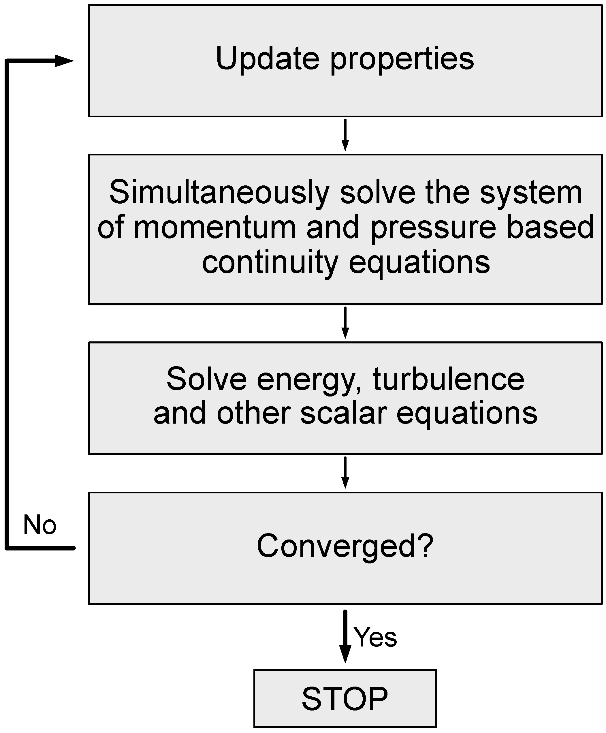
A pressure-based algorithm is implemented where conservation of mass is implicitly achieved through a pressure-based continuity equation, obtained by taking the divergent of the momentum Equation (
5) and introducing the condition
. A system of equations comprising this and the momentum equations is solved to obtain the velocity and pressure fields simultaneously. Energy and transport equations for turbulent variables are solved until convergence is reached.
In a collocated grid scheme, both the velocity and the pressure values needed for interpolation are retrieved from the same cell. However, when calculating the pressure field on a collocated grid, oscillations in the pressure field may appear as a result of an odd-even decoupling of the pressure and velocity, i.e., that on a specific point the pressure and velocity do not affect one another [
42]. As a result, a staggered grid method [
43] is used, where the velocity and pressure values are stored in different positions and for which the control volumes are no longer equal. Ultimately, the pressure values are calculated directly for the cell face, and no interpolation is needed. The decoupling of the pressure and velocity fields is eliminated along with any possible oscillations and is therefore used in the current work.
A hybrid initialization method is employed where the inlet velocity is set to
from
Table 1 and the absolute pressure at the outlet is set to
. The velocity and pressure fields calculated with this method are then introduced in the first cycle of the pressure-based algorithm. A flowchart of the numerical procedure is given in
Figure 5.
8. Results
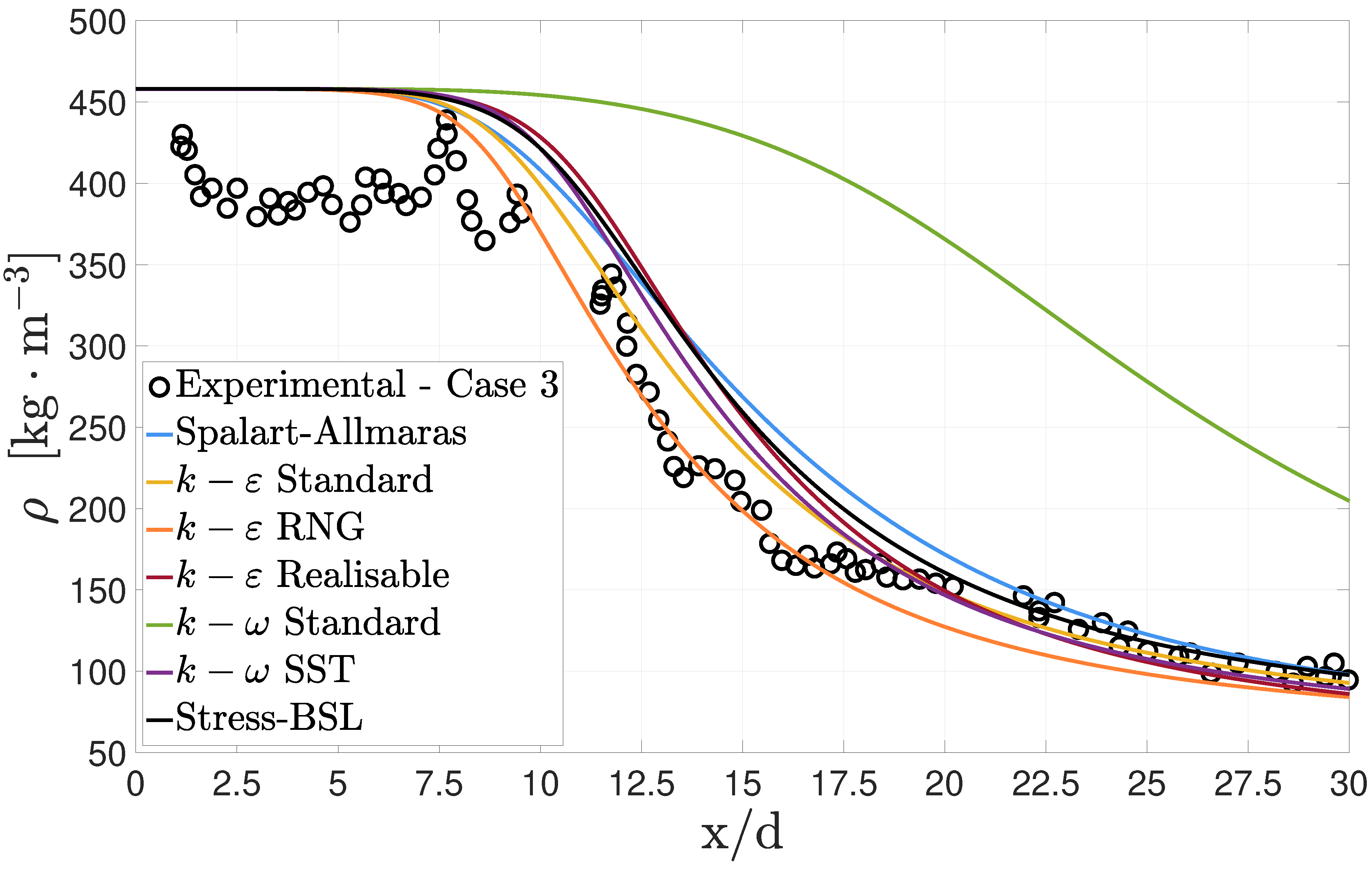
Figure 7 shows a comparison of the results obtained for the centerline density decay when using the turbulence models described for case 3. It is visible that almost all models predict a potential core with values ranging between
and
. The only exception is the standard
model that largely overestimates the length of the potential core to
, which can be attributed to the poor performance of this model in free-stream conditions. Even if the version here tested is an improvement over the 1998 Wilcox
model, with an added cross-diffusion term introduced specifically to deal with the free-stream sensitivity, it does not provide acceptable results throughout the whole of the domain.
The density values predicted in this region are higher than those of the experimental data, but this can be a result of the measuring procedure used by [
9]. Raman spectroscopy works by directing a monochromatic laser at the test substance and measuring the scattered radiation using a sensor. However, for higher densities, the jet tends to deflect the radiation along the axial direction, thus decreasing signal intensity at the sensor. As density reduces, this phenomenon is no longer predominant.
Turbulence seems not to influence the potential core. However, when entering the transition region, instabilities start to appear, and turbulent dissipation begins to increase. [
10] reports a maximum of density fluctuations in this region as pockets of dense fluid start to smear the potential core. The same authors also discuss how the heat absorbed to overcome the intermolecular attraction leads to an increase in the heat entropy production with a maximum already closer to the self-similar region. An analogy can be found between this and the trend of
and
.
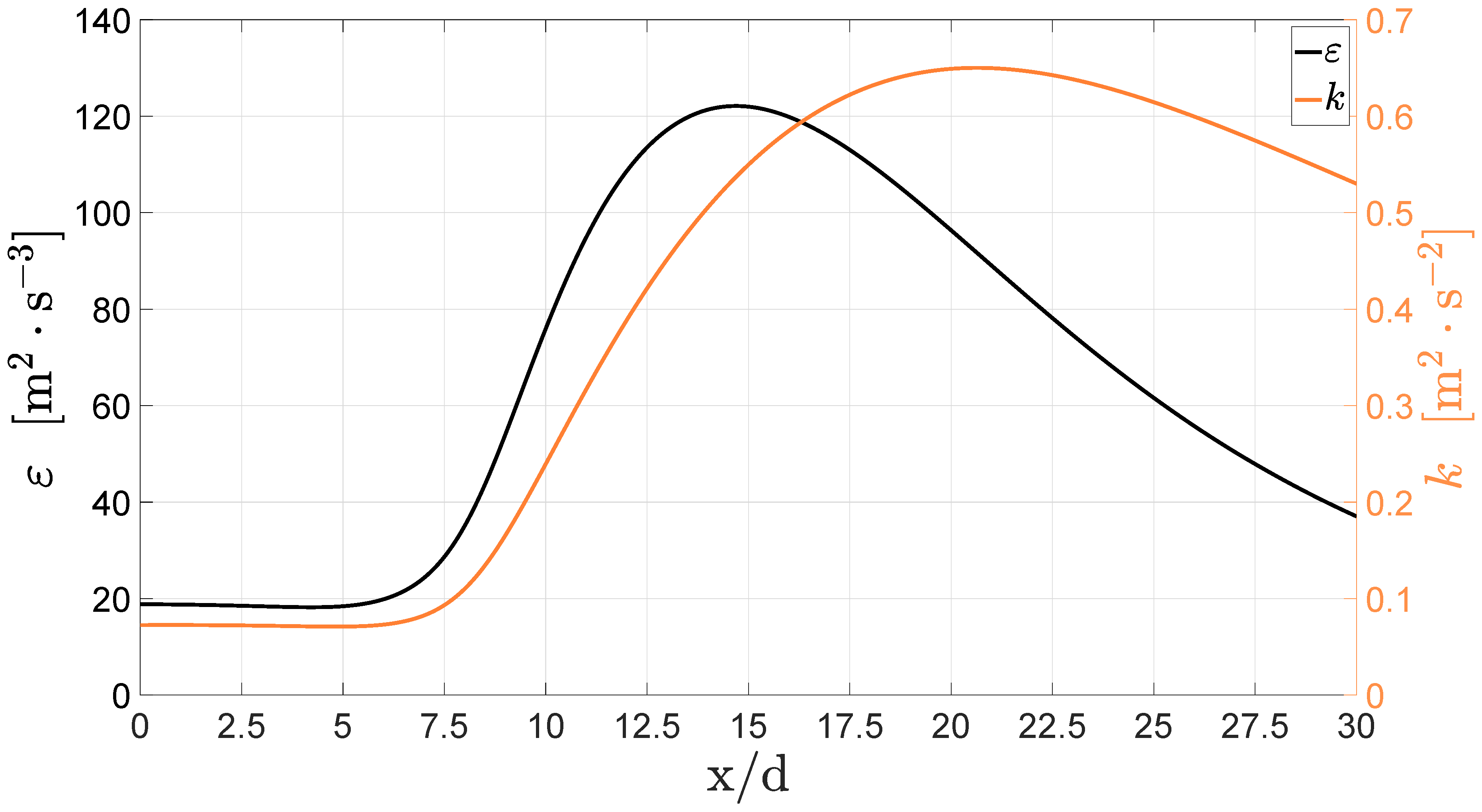
When this happens, the fluid crosses the pseudocritical line leading to thermal expansion and reduced shearing, resulting in turbulence dissipation, as depicted in
Figure 8, starting to decrease around
. This thermal expansion also appears to spawn sharp velocity fluctuations visible in the increase of turbulent kinetic energy, indicative of a robust turbulent mixing mechanism. The comparison of the maxima of
along the axial density evolution is seen in
Figure 9 for the RNG
model.
In this region, the more elaborate structure of the SST does not provide outstanding results despite having a shear-stress-based formulation for eddy viscosity. When moving away from the wall, returns to , and the model only uses the -based coefficients. Consequently, we can see that its results more closely match those of the variants than those of the standard model.
The five equation Stress-BSL model also overestimates the density values between , which could be related, in part, to the dependency of this model on and the inherent deficiencies of its transport equation. The one equation Spalart–Allmaras leads to a similar overestimation of density values between , but it is striking to see how well this simple formulation stacks against a five equation model.
In the three
based models, the realizable variant provides the worst results since the beginning of the transition zone up to
. It seems that the realisability constraint and the alternative
transport equation do not give any visible contribution. Between the standard and the RNG
, there are two main differences: the formulation for the destruction of the turbulent dissipation rate and the definition for the turbulent Prandtl number inserted into the energy equation and in the turbulent variables transport equations. Especially when considering the work from [
23], we are led to believe that the variable turbulent Prandtl number is the leading cause for an improved behavior of the RNG
model over the standard version. The model accurately predicts the density values across the domain.
In case 4, the differences in potential core length, depicted in
Figure 10, are similar to those of case 3, ranging from
to
with the standard
being once again the exception. Injection density is considerably reduced in this case when compared to that of case 3, and, as a consequence, there is no longer an apparent density overestimation in the potential core. However, an unrealistic potential core is still predicted independently of the turbulence model. In this case, the Stress-BSL model is the only one to correctly predict density values between
while the remaining provide a slight under prediction. Nevertheless, its behavior outside this region is not exceptional, and the overall results do not justify the additional computational cost. Results from the RNG
continue to be acceptable, but there is also an improvement from the standard
and the Spalart–Allmaras models for which the outcome is nearly identical. The decrease in the turbulence energy dissipation happens soon, at an
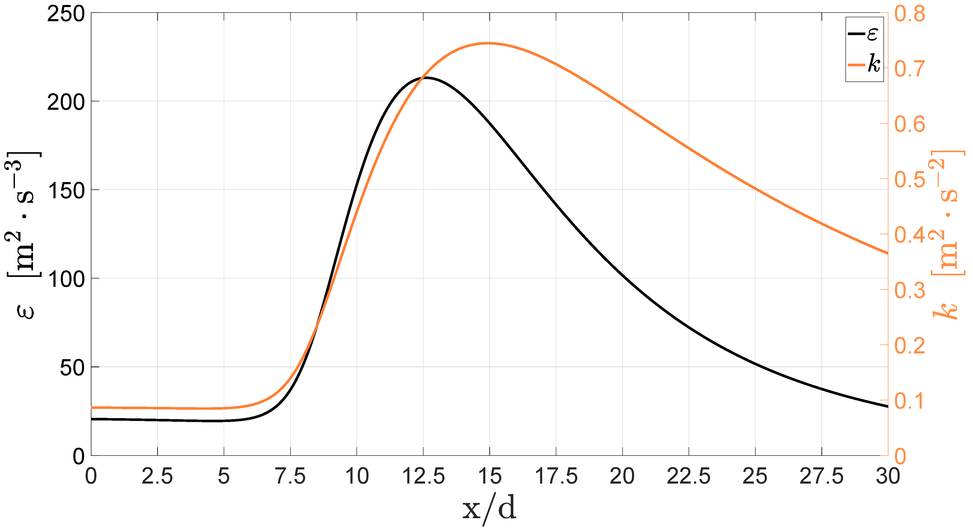
(
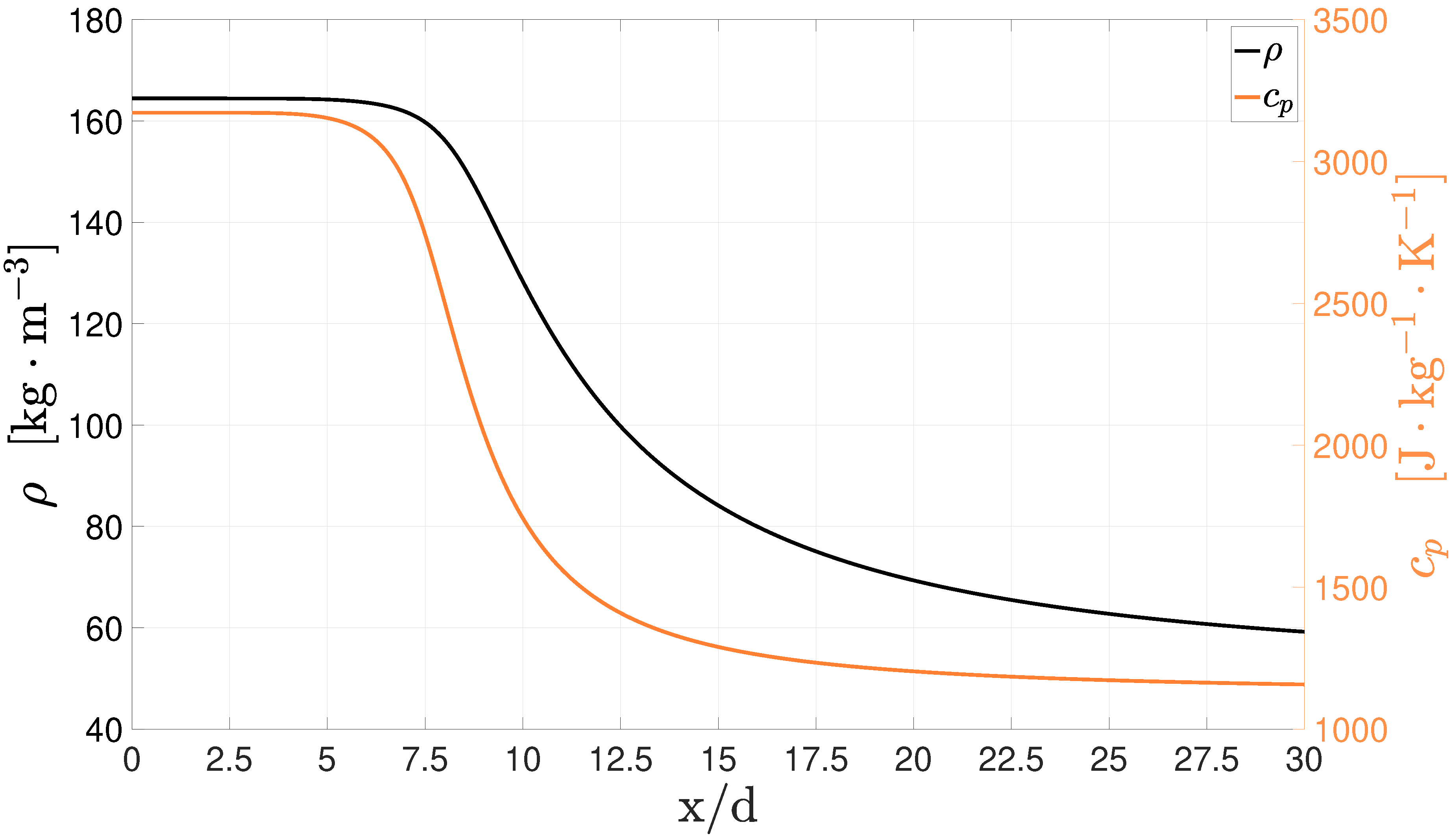
Figure 11) As it can be seen in
Figure 12, since the pseudo-boiling line is not crossed, there is not a peak in the
, which has an evolution in accordance to the axial density decay. The injection temperature of 137 K is already above the pseudo-boiling temperature, and there is no peak in the specific heat. remaining fairly constant until
5 along with the temperature inside the potential core, and begins then to decrease.
9. Conclusions
The steady-state Favre averaged governing equations are used to deal with the incompressible but variable-density flow that is characteristic of the current test cases. The system of equations is closed with six different models that are based either on the turbulent viscosity or the transport of the Reynolds stresses, to study the behavior of turbulence modeling in supercritical conditions.
An accurate formulation, capable of replicating the singular behavior of transport properties of supercritical fluids, is reviewed with detail. A pressure-based algorithm is used where the velocity and pressure fields are solved simultaneously. A staggered grid method is then implemented to prevent pressure fluctuations together with the QUICK scheme for the advective terms and second-order central differencing scheme for the diffusive terms.
The results obtained are compared to the experimental data for validation. There is a generally good agreement with the experimental data for both case 3 with the RNG model and for case 4 also with the RNG and with the Spalart–Allmaras model. Nevertheless, there is a clear distinction is that the results obtained from different turbulence models.
The results obtained with a second-order turbulence model show that there is no clear advantage in calculating higher-order turbulent correlation terms, indicating that their relevance under these conditions is minimal. Also, the blending functions and shear tress transport formulation for of the SST model do not contribute to improving predictions since the flow is mainly in a free-stream region. The RNG model, offers the best results for case 3, possibly due to the variable turbulent Prandtl number but the similarly good results obtained for case 4 with the Spalart–Allmaras and the Standard models indicate that there may be other relevant factors.
As a consequence, the results here obtained are indicative that there is no direct correlation between the turbulence model complexity and quality of the results, in what supercritical fluid flows are concerned. These results indicate that computational time can be gained with the use of simpler turbulence models. For this fact also contributes the pre-compiled real gas equation of state.
Having determined how the velocity field affects the flow structure, one of the next step is, therefore, to determine the impact of a heating mechanism inside the injector and the correct boundary conditions to be used.


