A Through-Life Cost Analysis Model to Support Investment Decision-Making in Concentrated Solar Power Projects


Abstract
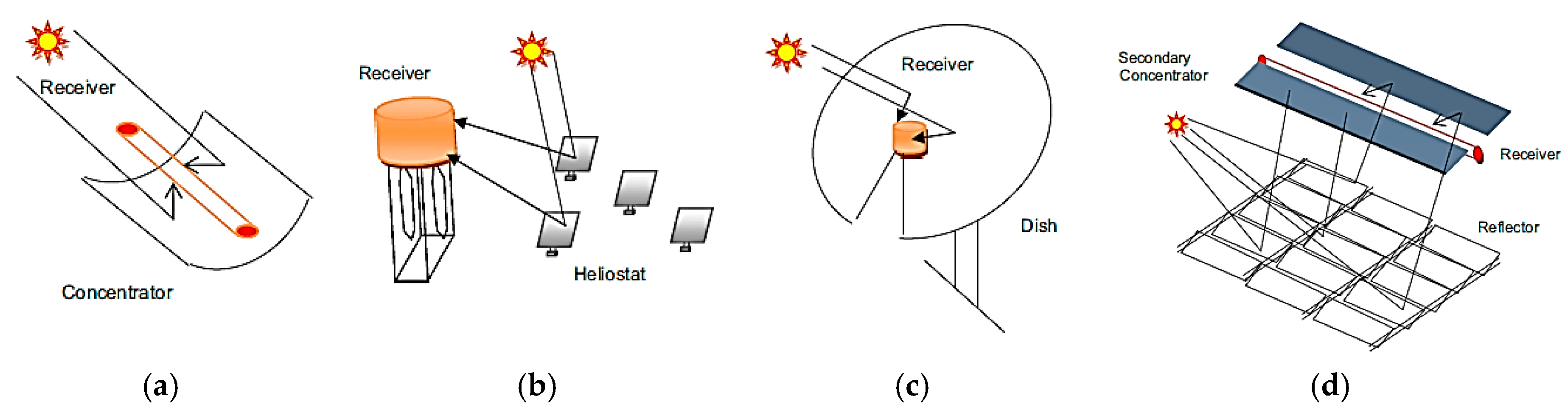
1. Introduction
2. Research Background
2.1. Financial Analysis Terminologies
2.2. Financial Metrics for CSP Projects
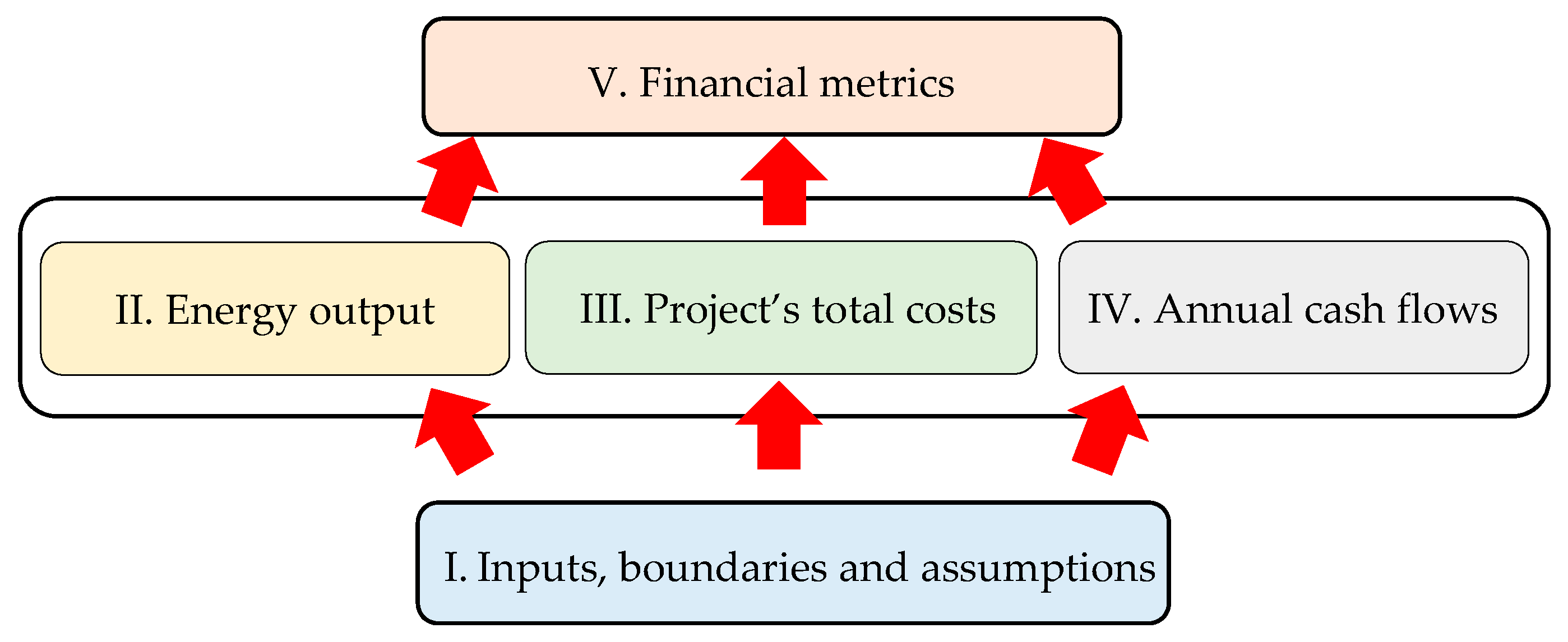
3. Proposed Methodology
- I)
- definition of input data, system boundaries and model assumptions;
- II)
- simulation of annual energy output;
- III)
- estimation of project’s total costs;
- IV)
- estimation of annual cash flows; and
- V)
- calculation of financial metrics.
3.1. Definition of Input Data, System Boundaries and Model Assumptions
- -
- No incentives are considered for this business.
- -
- Power purchase agreement (PPA) price and time of delivery (TOD) factors are constant throughout the project period, with a yearly 1% escalation in the price.
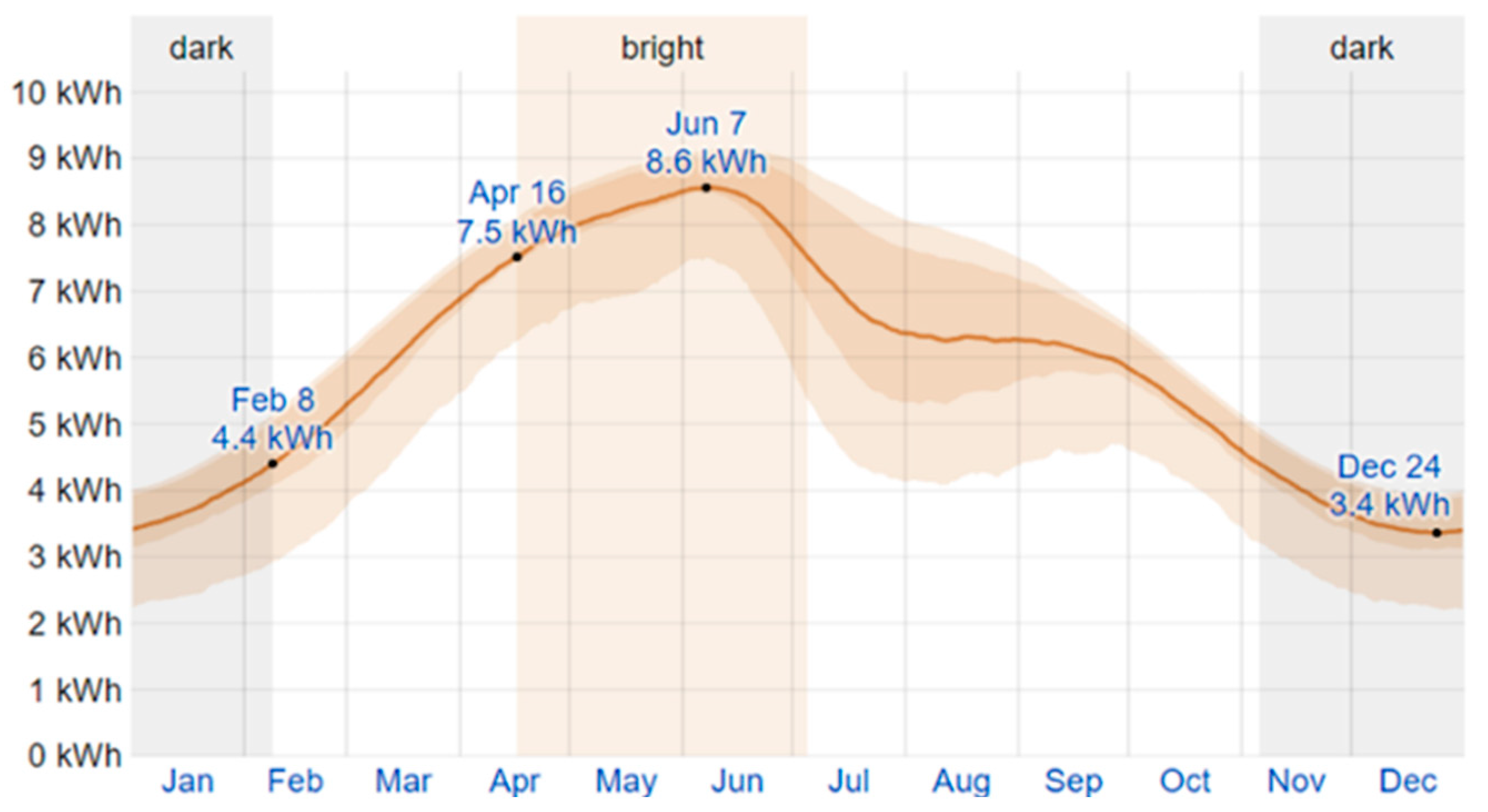
3.2. Simulation of The Annual Energy Output
3.3. Estimation of The Project’S Total Costs
3.4. Estimation of The Project’s Annual Cash Flows
3.5. Calculation of Output Metrics
4. Case Study
4.1. Geography and Topography
4.2. Weather Conditions and Temperature Variations
4.3. Energy Supply and Price of Electricity
4.4. Government’s Attitude Toward Solar Power
4.5. Solar Energy Potential
4.6. Input Data for SAM Simulations
| ● Latitude (decimal degrees). | ● Atmospheric pressure (mbar) |
| ● Longitude (decimal degrees). | ● Dry bulb temperature (°C) |
| ● Elevation above sea level (m). | ● Dew point temperature (°C) |
| ● Hour of the day | ● Wet bulb temperature (°C) |
| ● Diffuse horizontal radiation (W/m2) | ● Relative humidity (%) |
| ● Direct normal radiation (W/m2) | ● Wind velocity (m/s) |
| ● Global horizontal radiation (W/m2) | ● Wind direction (degrees) |
| ● Albedo | ● Snow depth |
4.7. Input Data for Financial Calculations
5. Results and Discussion
5.1. Financial Metrics
5.2. Financial Figures
5.3. Sensitivity Analysis
5.4. Model Validation
6. Conclusions and Future Work
Author Contributions
Acknowledgments
Conflicts of Interest
References
- International Energy Agency (IEA). Renewables 2019: Analysis and Forecasts to 2024; OECD Publishing: Paris, France; Available online: https://webstore.iea.org/market-report-series-renewables-2019 (accessed on 6 January 2020).
- Bhattarai, S.; Kafle, G.K.; Euh, S.-H.; Oh, J.-H.; Kim, D.H. Comparative study of photovoltaic and thermal solar systems with different storage capacities: Performance evaluation and economic analysis. Energy 2013, 61, 272–282. [Google Scholar] [CrossRef]
- Chaanaoui, M.; Vaudreuil, S.; Bounahmidi, T. Benchmark of concentrating solar power plants: Historical, current and future technical and economic development. Procedia Comput. Sci. 2016, 83, 782–789. [Google Scholar] [CrossRef]
- Mehta, A.; Kapoor, A.; Neopaney, H.K. Conceptual design of concentrated solar power plant using SPT-Solar power tower technology. In Proceedings of the International Symposium on Aspects of Mechanical Engineering and Technology for Industry, Itanagar, India, 6–8 December 2014; Volume 2. [Google Scholar]
- Au, T.; Au, T.P. Engineering Economics for Capital Investment Analysis, 2nd ed.; Prentice-Hall, Inc.: Upper Saddle River, NJ, USA, 1992. [Google Scholar]
- Shafiee, M.; Brennan, F.; Armada Espinosa, I. A parametric whole life cost model for offshore wind farms. Int. J. Life Cycle Assess. 2016, 21, 961–975. [Google Scholar] [CrossRef]
- Ghosh, C.; Maiti, J.; Shafiee, M.; Kumaraswamy, K.G. Reduction of life cycle costs for a contemporary helicopter through improvement of reliability and maintainability parameters. Int. J. Qual. Reliab. Manag. 2018, 35, 545–567. [Google Scholar] [CrossRef]
- Animah, I.; Shafiee, M.; Simms, N.; Erkoyuncu, J.A.; Maiti, J. Selection of the most suitable life extension strategy for ageing offshore assets using a life-cycle cost-benefit analysis approach. J. Qual. Maint. Eng. 2018, 24, 311–330. [Google Scholar] [CrossRef]
- Dale, M. A comparative analysis of energy costs of photovoltaic, solar thermal, and wind electricity generation technologies. Appl. Sci. 2013, 3, 325–337. [Google Scholar] [CrossRef]
- Mahlangu, N.; Thopil, G.A. Life cycle analysis of external costs of a parabolic trough Concentrated Solar Power plant. J. Clean. Prod. 2018, 195, 32–43. [Google Scholar] [CrossRef]
- Zhao, Z.-Y.; Chen, Y.-L.; Thomson, J.D. Levelized cost of energy modeling for concentrated solar power projects: A China study. Energy 2017, 120, 117–127. [Google Scholar] [CrossRef]
- Yang, S.; Zhu, X.; Guo, W. Cost-benefit analysis for the concentrated solar power in China. J. Electr. Comput. Eng. 2018, 4063691. [Google Scholar] [CrossRef]
- Cogliani, E. The role of the direct normal irradiance (DNI) forecasting in the operation of solar concentrating plants. Energy Procedia 2014, 49, 1612–1621. [Google Scholar] [CrossRef]
- Short, W.; Packey, D.; Holt, T. A Manual for the Economic Evaluation of Energy Efficiency and Renewable Energy Technologies; NREL/TP-462-5173; National Renewable Energy Laboratory (NREL): Golden, CO, USA, 2005.
- Kumar, R. Valuation: Theories and Cozncepts, 1st ed.; Academic Press: Cambridge, MA, USA, 2015; 514p. [Google Scholar]
- Luo, J. Engineering, Financial and Net Energy Performance, and Risk Analysis for Parabolic Trough Solar Power Plants. Ph.D. Thesis, Texas A&M University, College Station, TX, USA, 2014. [Google Scholar]
- Babbei, D.F.; Merrill, C.B. Valuation of Interest-Sensitive Financial Instruments: SOA Monograph M-F196-1; Society of Actuaries: Schaumburg, IL, USA, 1996. [Google Scholar]
- Zala, J.N.; Jain, P. Design and optimization of a biogas-solar-wind hybrid system for decentralized energy generation for rural India. Int. Res. J. Eng. Technol. 2017, 4, 649–656. [Google Scholar]
- Pugh, P.G. Working top-down: Cost estimating before development begins. Proc. Inst. Mech. Eng. Part G 1992, 206, 143–151. [Google Scholar] [CrossRef]
- Hooshmand, Y.; Köhler, P.; Korff-Krumm, A. Cost estimation in engineer-to-order manufacturing. Open Eng. 2016, 6, 22–34. [Google Scholar] [CrossRef]
- Mendelsohn, M.; Kreycik, C.; Bird, L.; Schwabe, P.; Cory, K. The Impact of Financial Structure on the Cost of Solar Energy; NREL/TP-6A20-53086; National Renewable Energy Laboratory: Golden, CO, USA, 2012.
- Dobos, A.; Neises, T.; Wagner, M. Advances in CSP simulation technology in the System Advisor Model. Energy Procedia 2014, 49, 2482–2489. [Google Scholar] [CrossRef]
- City of Tucson. Available online: http://www.cityoftucson.org/ (accessed on 30 September 2018).
- Google Maps. Available online: https://www.google.co.uk/maps (accessed on 30 September 2018).
- Turchi, C. Parabolic trough Reference Plant for Cost Modeling with the Solar Advisor Model (SAM); Technical Report NREL/TP-550-47605; National Renewable Energy Lab.: Golden, CO, USA, 2010.
- Bracken, N.; Macknick, J.; Tovar-Hastings, A.; Komor, P.; Gerritsen, M.; Mehta, S. Concentrating Solar Power and Water Issues in the U.S. Southwest; Technical Report NREL/TP-6A50-6137; National Renewable Energy Lab.: Golden, CO, USA, 2015.
- Encyclopædia Britannica. 2018. Available online: https://www.britannica.com/place/Tucson (accessed on 19 August 2018).
- The Typical Weather Anywhere on Earth, Weather Spark. Available online: https://weatherspark.com/ (accessed on 30 September 2018).
- U.S. Energy Information Administration (EIA). Arizona-State Energy Profile Overview. 2018. Available online: https://www.eia.gov/state/?sid=AZ (accessed on 19 August 2018).
- Electricity Local. Tucson, AZ Electricity Rates. 2018. Available online: https://www.electricitylocal.com/states/arizona/tucson/. (accessed on 6 January 2020).
- Pool, S.; Coggin, J.D.P. Fulfilling the promise of concentrating solar power. Center for American Progress. 2013. Available online: https://www.americanprogress.org/ (accessed on 6 January 2020).
- Tucson Electric Power (TEP). Real-time Solar and Wind Generation. 2020. Available online: https://www.tep.com/solar-dashboard/ (accessed on 6 January 2020).
- Ren, L.Z.; Zhao, X.G.; Yu, X.X.; Zhang, Y.Z. Cost-benefit evolution for concentrated solar power in China. J. Clean. Prod. 2018, 190, 471–482. [Google Scholar]
- International Renewable Energy Agency (IRENA). Renewable Energy Technologies: Cost Analysis Series, Concentrating Solar Power; IRENA Working Paper; IRENA: Abu Dhabi, UAE, 2012; Volume 1. [Google Scholar]


| No. | Input Description | Value |
|---|---|---|
| 1 | Location | Tucson city, Arizona state, US |
| 2 | Plant type | Parabolic trough |
| 3 | Power rating of the plant | 50MW |
| 4 | Number of solar collector assemblies per loop | 14 |
| 5 | Collector type | Solargenix SGX-1 (SAM collector library) |
| 6 | Receiver type | Schott PTR70 2008 (SAM receiver library) |
| 7 | Field heat transfer fluid | Hitec Solar Salt |
| 8 | Design loop outlet temp (C°) | 550 |
| 9 | Design gross output (MWe) | 167 |
| 10 | Estimated gross to net conversion factor | 90%, where parasitic losses typically reduce net output by this percentage of the design gross power |
| 11 | Condenser type | Air-cooled |
| 12 | Full load hours of TES (hours) | 6 |
| 13 | Parallel tank pairs | 2 |
| 14 | Tank height (meters) | 15 |
| 15 | Number of field subsections | 8 |
| No. | Input Description | Value |
|---|---|---|
| 1 | Annual energy output (kWh) | 456,351,232 (Derived from the SAM) |
| 2 | Analysis period (years) | 25 |
| 3 | Loan amount (Total installed cost) ($) | 794,177,280.00 |
| 4 | Loan interest rate (%) | 4 |
| 5 | Inflation rate (%)/year | 2.5 |
| 6 | Nominal discount rate (%)/year | 8.1375 |
| 7 | Insurance rate (%)/year of installed cost | 0.5 |
| 8 | Debt closing costs ($) | 450,000 |
| 9 | PPA price (cent/kWh) | 16 |
| 10 | PPA price escalation (%/year) | 1 |
| 11 | Tenor (years) | 18 |
| 12 | Investment Tax credit (%) | 30 |
| 13 | Incentives | No incentives |
| 14 | Time of delivery factor (TOD) | 1 for all periods |
| 15 | Salvage value | 0 |
| Financial Metric | Value |
|---|---|
| Annual Energy Output (kWh) | 456,351,232 |
| Net present value (NPV) ($) | 64,122,737.29 |
| Internal rate of return (IRR) (%) | 12 |
| Discounted payback period (DPBP) (Years) | 17.24 |
| Benefit/Cost ratio (BCR) | 1.15 |
| Total life-cycle cost (TLCC) ($) | 773,304,457.05 |
| LCoE (cent/kWh) | 16.06 |
| Output Financial Metric | The Created Financial Model (Excel Spreadsheet) | SAM Tool | Difference (%) |
|---|---|---|---|
| Energy output (kWh) | 456,351,232 | 456,351,232 | 0 |
| LCoE ($/kWh) | 0.16 | 0.16 | 0 |
| NPV ($) | 64,123,099.54 | 64,192,692 | 0.12% |
| IRR (%) | 12 | 10.28 | 16.7% |
| TLCC ($) | $773,304,457.05 | 876,886,464 | 11.8% |
| DPBP (year) | 17.24 | 20 | 13.8% |
© 2020 by the authors. Licensee MDPI, Basel, Switzerland. This article is an open access article distributed under the terms and conditions of the Creative Commons Attribution (CC BY) license (http://creativecommons.org/licenses/by/4.0/).
Share and Cite
Shafiee, M.; Alghamdi, A.; Sansom, C.; Hart, P.; Encinas-Oropesa, A. A Through-Life Cost Analysis Model to Support Investment Decision-Making in Concentrated Solar Power Projects. Energies 2020, 13, 1553. https://doi.org/10.3390/en13071553
Shafiee M, Alghamdi A, Sansom C, Hart P, Encinas-Oropesa A. A Through-Life Cost Analysis Model to Support Investment Decision-Making in Concentrated Solar Power Projects. Energies. 2020; 13(7):1553. https://doi.org/10.3390/en13071553
Chicago/Turabian StyleShafiee, Mahmood, Adel Alghamdi, Chris Sansom, Phil Hart, and Adriana Encinas-Oropesa. 2020. "A Through-Life Cost Analysis Model to Support Investment Decision-Making in Concentrated Solar Power Projects" Energies 13, no. 7: 1553. https://doi.org/10.3390/en13071553
APA StyleShafiee, M., Alghamdi, A., Sansom, C., Hart, P., & Encinas-Oropesa, A. (2020). A Through-Life Cost Analysis Model to Support Investment Decision-Making in Concentrated Solar Power Projects. Energies, 13(7), 1553. https://doi.org/10.3390/en13071553