Monte Carlo-Based Procedure for Determining the Maximum Energy at the Output of Accelerometers

Abstract

The solutions presented in this paper can be the basis for mutual comparison of different types of accelerometers produced by competing companies. An application of a procedure based on the Monte Carlo method to determine the maximum energy at the output of accelerometers is discussed here. The fixed-point algorithm controlled by the Monte Carlo method is used to determine this energy. This algorithm can only be used for the time-invariant and linear measurement systems. Hence, the accelerometer nonlinearities are not considered here. The mathematical models of the accelerometer and the special filter, represented by the relevant transfer functions, are the basis for the above procedure. Testing results of the voltage-mode accelerometer of type DJB A/1800/V are presented here as an example of an implementation of the solutions proposed. Calculation of the energy was executed in Mathcad 14 program with the built-in Programming Toolbar. The value of the maximum output energy determined for a specified time interval corresponds to the maximum integral-square error of the accelerometer. Such maximum energy can be a comparative ratio just like the accuracy class in the case of instruments used for the static measurements. Hence, the main analytical and technical contributions of this paper concern the development of theoretical procedures and the presentation of their application on the example of a real type of accelerometer.

1. Introduction

The basic condition for mutual comparison of different types of accelerometers [1,2,3] is that the accelerometers under test have the same frequency bandwidth and it is necessary to develop the model of special filter [4] which is the reference for such an analysis. The frequency bandwidth of the filter must be the same as the operation frequency range of the compared accelerometers.

The reference of energies at the outputs of the accelerometer and the filter is necessary because, from the point of view of the practical implementation of measurements, only the value of energy for the operation range of the accelerometer, not for the full frequency bandwidth, is interesting [5]. Such comparison is carried out by subtracting the energy value at the outputs of both accelerometers. The difference between these energies is defined below as the reference energy and, for the purpose of determining its maximum value, it is convenient to apply the algorithm discussed in Section 3.

The reference energy of an accelerometer corresponds to the integral-square error [6] of the sensor related to this type of error at the output of the special filter. Developing the procedure determines the maximum value of the integral-square error (maximum reference energy) and seems to be the justified proposal for the comparison of different accelerometers.

The basis for the implementation of the task described above is the mathematical model of the accelerometer determined through its parametric identification [7,8,9,10,11,12], as well as the mathematical model of the special filter. The model of the accelerometer is defined by the second-order transfer function [1,2,3], whereas the model of the filter should be a high-order (a range of 10 to 15 order is sufficient). Determination of the parameters of the accelerometer model should be carried out on the basis of measurement points of both components of the frequency response (the amplitude and phase) in accordance with the procedures included in the relevant international guides [7]. In this way (e.g., by using the weighted least squares procedure (WLSP)), the accelerometer parameters and associated uncertainties can be obtained [3,13,14]. Additionally, when we want to determine the associated uncertainties, it is necessary to use the Monte Carlo procedure (MCP) [15,16,17,18], whose number of trials can be assumed in advance according to the guidelines included in the JCGM (Joint Committee for Guides in Metrology)—supplement 1 [13]. The model of the filter is expected to meet the so-called non-distortion transformation [19], according to which the amplitude-frequency and phase-frequency responses are flat and linear, respectively, within the frequency bandwidth of interest [20]. However, these assumptions are ideal from a practical point of view. In practice, they are not possible to meet, and one can only strive to attain them [20], for example, by using the above-mentioned high-order filter. The degree of achievement for the approximation therefore depends on the type of filter used and has an effect on the value of the reference energy (i.e., the higher the order of the approximation, the lower value of this energy). Hence, there is the obvious necessity to use the same model of the filter within the considered comparison of the different types of accelerometers.

The maximum value of the reference energy can be determined by using the fixed-point algorithm (FPA) [5,21,22,23] with its extension by the MCP [13,18]. The MCP can be implemented based on the same assumptions as in the case of the procedure intended for determining the uncertainties associated with the parameters of the accelerometer model by using the WLSP. A method based on a system of complex convolution equations could also be applied instead of the above-mentioned FPA [4]. However, the possibilities of its application are limited due to the numerical difficulties of solving a system including more than twenty-five equations [24]. Therefore, for the needs of this paper, the first type of approach is chosen. This choice is also supported by the fact that by employing the FPA, the maximum reference energy can be obtained quickly. The FPA also allows determination of the critical case of the input signal of the accelerometer that is limited both in magnitude and in time interval [25], and which produces this energy. Both the number of reversals of such a signal and the times at which this reversal occurs are determined. It should be emphasized here that any other signal contained in these limits generates less energy than that produced by the critical case of the magnitude-limited signal [4].

The FPA determines, by an application of the MCP, the numerical value of the maximum reference energy in an iterative way for the ranges of variability of the model parameter of the accelerometer by the values of associated uncertainties [26,27]. Taking into account the uniform distribution of parameters in the above ranges, the Monte Carlo simulation (MCS) should therefore be based on a uniform pseudo-random number generator [28].

The assessment of the impact of the uncertainties associated with the parameters of the accelerometer on the value of the absolute error is presented in studies by Tomczyk [26,27]. However, this assessment does not apply to full ranges of parameter variability on the values of uncertainties associated with them. Additionally, the cited assessment concerns only the values of parameters increased or decreased by the values of the uncertainties associated with them. Therefore, it was not necessary to use the MCP in such a case.

The above-mentioned issues are developed in this paper using the MCP. The block diagrams with an exact description of both the proposed MCP as well as the algorithm for determining the maximum reference energy at the output of accelerometers are discussed here. This maximum reference energy can be the basis for mutual comparison [4] of accelerometers with the same bandwidth but produced by different companies. This comparison relates to the maximum integral-square error, which reflects an accuracy of the accelerometer. It can therefore help one choose the proper accelerometer from many types at different prices.

The practical solutions presented here are applied to the testing of the DJB A/1800/V type of accelerometer [29].

2. Accelerometer Modeling

The model of the accelerometer is defined by using the transfer function,

$$K\left(s\right)=\frac{S_{\mathrm{a}}{\omega }_0^2}{s^2+2\beta {\omega }_{0}s+{\omega }_0^2},$$

(1)

where $S_{\mathrm{a}}$ and $\beta$ are the accelerometer voltage sensitivity and damping factor, respectively, while ${\omega }_0=2\pi f_0,$ where $f_0$ denotes the non-damped natural frequency.

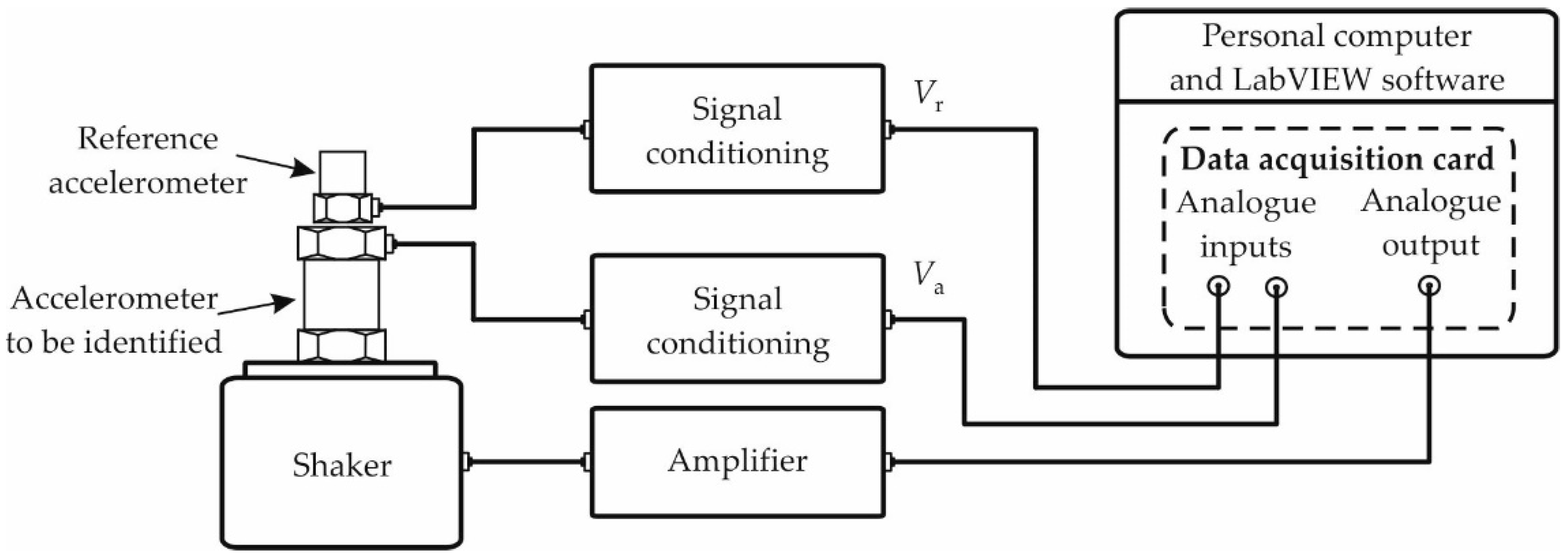
Parametric identification of the accelerometer model is directed towards determining the parameters of the transfer function given by Equation (1) together with associated uncertainties [8,9]. The first step in this subject is the determination of the measurement points for both frequency responses. This is achieved by applying the back-to-back method commonly used in the measurement practice. The block diagram for this type of identification method is shown in Figure 1. The reference accelerometer is used here as the comparison signal source, while the data acquisition card together with the LabVIEW software are employed for the control of the shaker and recording of the measurement data.

The sensitivity $S_{\mathrm{a}}$ of the tested accelerometer is determined on the basis of the relation,

$$S_{\mathrm{a}}=S_r\frac{V_{\mathrm{a}}}{V_{\mathrm{r}}},$$

(2)

where $S_{\mathrm{r}}$, $V_{\mathrm{a}}$, and $V_{\mathrm{r}}$ are the sensitivity of the reference accelerometer, the voltage output of the system for signal conditioning at the output of the accelerometer, and the voltage output of the reference, respectively.

Based on the measurement points of the frequency responses of the accelerometer, the estimates ${\tilde{S}}_{\mathrm{a}}$, ${\tilde{f}}_0,$ and $\tilde{\beta }$ are associated with the parameters $S_{\mathrm{a}}$, $f_0,$ and $\beta$ which occur in the transfer function given by Equation (1), as well as the associated uncertainties $u\left({\tilde{S}}_{\mathrm{a}}\right)$, $u\left({\tilde{f}}_0\right),$ and $u\left(\tilde{\beta }\right)$, which are determined by applying the WLSP [3,13]. This procedure employs the MCP which utilizes the Box–Muller and the Wichmann–Hill pseudo-random number generator with normal and uniform distributions, respectively. The minimum number $M$ of Monte Carlo trials (MCts) should be determined based on the relation,

$$M>\frac{{10}^4}{1-p},$$

(3)

where $p$ denotes the assumed coverage probability [13].

3. Algorithm for Determining the Maximum Energy (ME)

The optimization algorithm for determining the ME is based on the integral equation,

$${\int }_0^{T}x\left(v\right)\Phi \left(\tau ,v\right)dv=\xi ·x\left(\tau \right),$$

(4)

where

$$\begin{array}{c}\Phi \left(\tau ,v\right)={\Phi }_{\mathrm{a}}\left(\tau ,v\right)-{\Phi }_{\mathrm{f}}\left(\tau ,v\right)={\int }_0^T{k}_{\mathrm{a}}\left(t-\tau \right)k_{\mathrm{a}}\left(t-v\right)dt+\\ -{\int }_0^T{k}_{\mathrm{f}}\left(t-\tau \right)k_{\mathrm{f}}\left(t-v\right)dt, t\in \left(0,T\right),\end{array}$$

(5)

while $x\left(t\right)$ is any signal at the input of the accelerometer, $\xi$ is the Lagrange multiplier [5], $k_{\mathrm{a}}\left(t\right)$ and $k_{\mathrm{f}}\left(t\right)$ are the impulse responses of the accelerometer and the filter, respectively, and $T$ denotes the time of accelerometer testing. The impulse responses $k_{\mathrm{a}}\left(t\right)$ and $k_{\mathrm{f}}\left(t\right)$ are determined as the inverse Laplace transforms of the corresponding transfer functions $K_{\mathrm{a}}\left(s\right)$ and $K_{\mathrm{f}}\left(s\right)$. In turn, the transfer function $K_{\mathrm{a}}\left(s\right)$ is obtained by way of the parametric identification of the accelerometer, while the transfer function $K_{\mathrm{f}}\left(s\right)$ is convenient to be defined by the low-pass Butterworth filter given by,

$$K_{\mathrm{f}}\left(s\right)=\frac{S_{\mathrm{a}}}{{\prod }_{i=1}^L\left(\frac{s}{2\pi f_{\mathrm{c}}}-e^{\frac{\mathrm{j}\left(2i+L-1\right)\mathsf{\pi }}{2L}}\right)}.$$

(6)

In Equation (6), L is the order of the filter, $f_{\mathrm{c}}$ is the filter’s cut-off frequency, which is equal to the frequency bandwidth of the accelerometer, and $\mathrm{j}$ denotes the imaginary number.

The solution to Equation (4) determines the signal $x_{\mathrm{m}}\left(t\right)$ that yields the maximum value of the coefficient $\xi$ for which the ratio is satisfied,

$$\xi \left(x,y\right)=\frac{E\left(y\right)}{E\left(x\right)}$$

(7)

where $E\left(x\right)$ and $E\left(y\right)$ are the energies of any input and output signals $x\left(t\right)$ and $y\left(t\right),$ respectively. The error $y\left(t\right)$ is defined by,

$$y\left(t\right)=y_{\mathrm{a}}\left(t\right)-y_{\mathrm{f}}\left(t\right),$$

(8)

where

$$y_{\mathrm{a}}\left(t\right)={\int }_0^t{k}_{\mathrm{a}}\left(t-\tau \right)x\left(\tau \right)d\tau$$

(9)

and

$$y_{\mathrm{f}}\left(t\right)={\int }_0^t{k}_{\mathrm{f}}\left(t-\tau \right)x\left(\tau \right)d\tau$$

(10)

are the output signals of the accelerometer and filter, respectively.

Both the signal $x\left(t\right)$ as well as the signal $x_{\mathrm{m}}\left(t\right),$ maximizing the coefficient $\xi ,$ are limited in time $T$ and magnitude $a$. Thus, we can write,

$$x\left(t\right)\le a,\hspace{1em}{x}_{\mathrm{m}}\left(t\right)\le a.$$

(11)

The denominator and nominator of Equation (7) are represented by,

$$E\left(x\right)={\int }_0^T{\left[x\left(t\right)\right]}^{2}dt,$$

(12)

and

$$E\left(y\right)=E\left(y_{\mathrm{a}}\right)-E\left(y_{\mathrm{f}}\right)={\int }_0^T{\left[y_{\mathrm{a}}\left(t\right)\right]}^{2}dt-{\int }_0^T{\left[y_{\mathrm{f}}\left(t\right)\right]}^{2}dt={\int }_0^T{\left[y\left(t\right)\right]}^{2}dt.$$

(13)

Substituting Equations (9) and (10) into Equation (13) and taking into account the relationship between the impulse responses,

$$k\left(t\right)=k_{\mathrm{a}}\left(t\right)-k_{\mathrm{f}}\left(t\right)={ℒ}^{-1}\left[K_{\mathrm{a}}\left(s\right)\right]-{ℒ}^{-1}\left[K_{\mathrm{f}}\left(s\right)\right],$$

(14)

we finally have

$$E\left(y\right)={\int }_0^T{\left[{\int }_0^{t}k\left(t-\tau \right)x\left(\tau \right)d\tau \right]}^{2}dt.$$

(15)

When the signal $x\left(t\right)$ is limited in magnitude $M$ (i.e., it has a rectangular shape), then we can consider the condition given by,

$$a·\mathrm{sgn}\left[{\int }_0^{T}x\left(v\right)\Phi \left(\tau ,v\right)dv\right]=\xi x\left(\tau \right)$$

(16)

where $\mathrm{sgn}$ denotes the signum operation.

Hence, the signal maximizing the energy $E\left(y\right)$ is represented by,

$$x_{\mathrm{m}}\left(\tau \right)=\frac{a·\mathrm{sgn}\left[{\int }_0^{T}x\left(v\right)\Phi \left(\tau ,v\right)dv\right]}{{\xi }_{\max }}$$

(17)

and ${\xi }_{\max }$ is the maximum value of $\xi \left(x,y\right)$ defined by Equation (7).

The procedure for determining the input signal that maximizes the energy $E\left(y\right)$ is based on the FPA [5] and includes the following stages:

• Calculate the function $\Phi \left(\tau ,v\right)$ based on Equation (5);
• Determine the initial input signal $x^0\left(\tau \right),$ where ${\xi }^0$ is the initial Lagrange multiplier, assumed in advance by the formula,

  $$x^0\left(\tau \right)=\frac{a·\mathrm{sgn}\left[\Phi \left(\tau ,v\right)\right]}{{\xi }^0}$$

  (18)
• Determine the maximizing signal on the basis of the iterative algorithm, given by,

  $$\begin{array}{c}{x}^{i+1}\left(\tau \right)=\frac{a·\mathrm{sgn}\left[{\int }_0^T{x}^i\left(v\right)\Phi \left(\tau ,v\right)dv\right]}{{\xi }_{i+1}}\\ \mathrm{for}\hspace{1em}i=0, 1, 2, \dots , J-1,\end{array}$$

  (19)

  where $J$ denotes the number of assumed iterations.
  It should be emphasized that for each iteration step $i,$ the Lagrange multiplier ${\xi }_{i+1}$ must be determined based on Equation (7).
• Calculate the energy $E\left(y\right)$ by using Equation (15).

The signal $x_{\mathrm{m}}\left(t\right)$ that yields the maximum value of the quotient $\xi \left(x,y\right)$ is the one that maximizes the energy $E\left(y\right).$ This ME denoted by $E^{\max }\left(y\right)$ is obtained by substituting the signal $x_{\mathrm{m}}\left(t\right)$ into Equation (15). Then, we have

$$E^{\max }\left(y\right)={\int }_0^T{\left[{\int }_0^{t}k\left(t-\tau \right)x_{\mathrm{m}}\left(\tau \right)d\tau \right]}^{2}dt$$

(20)

The energy $E^{\max }\left(y\right)$ is the accelerometer output energy, referred to as the output energy of filter, and is valid for the accelerometer frequency bandwidth.

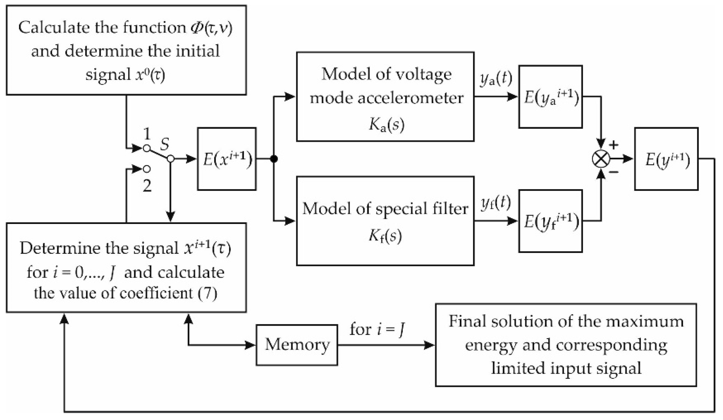
Figure 2 shows the block diagram of the algorithm described above applied for determining the ME at the output of accelerometers. The switch S has the position 1 for $i=0$, and it has the position 2 when $i>0$. During the particular iterations i = 1, 2, …, J$-$1 of the algorithm above, the energies $E\left(y^i\right)$ and $E\left(y^{i-1}\right)$ are compared with each other, and the value of the current ME and the corresponding input signal limited in magnitude are stored in the memory. This signal can be then processed by using specialized IT tools, e.g., neural network [30].

The final solutions of the ME and corresponding signal are delivered for $i=J-1$. It should be noted that this algorithm converges quickly because the maximum number J of iterations does not exceed 30.

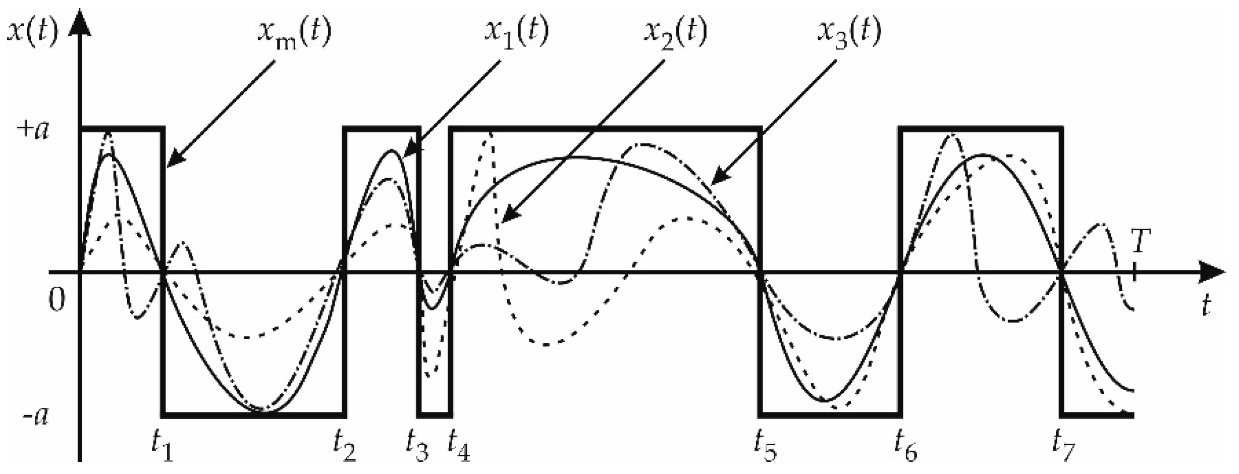
The signal producing the ME has the property that any other signal contained in its limitations can only yield less energy than the energy value caused by the maximizing signal [4]. Figure 3 shows examples of the maximizing signal $x_{\mathrm{m}}\left(t\right)$ limited simultaneously in time and magnitude and three other signals $x_1\left(t\right)$, $x_2\left(t\right),$ and $x_3\left(t\right)$ contained in its limitations denoted by $\pm a$ (magnitude) and $T$ (time).

The limited signal $x_{\mathrm{m}}\left(t\right)$ in Figure 3 has seven time switches denoted by $t_1$, $t_2$, …, $t_7$. The number of these switches and the times at which they occur are determined by the FPA, and they constitute the shape of the signal that maximizes the energy at the output of the accelerometer.

4. Monte Carlo-Based Procedure for Determining the ME

On the basis of obtaining both estimates ${\tilde{S}}_{\mathrm{a}}$, ${\tilde{f}}_0,$ and $\tilde{\beta }$ of the accelerometer model and the associated uncertainties $u\left({\tilde{S}}_{\mathrm{a}}\right)$, $u\left({\tilde{f}}_0\right),$ and $u\left(\tilde{\beta }\right)$, the values of the parameters denoted by ${\tilde{S}}_{\mathrm{a}}^{\max }$, ${\tilde{f}}_0^{\max },$ and ${\tilde{\beta }}^{\max }$ that produce the energy $E^{\max }\left(y\right)$ 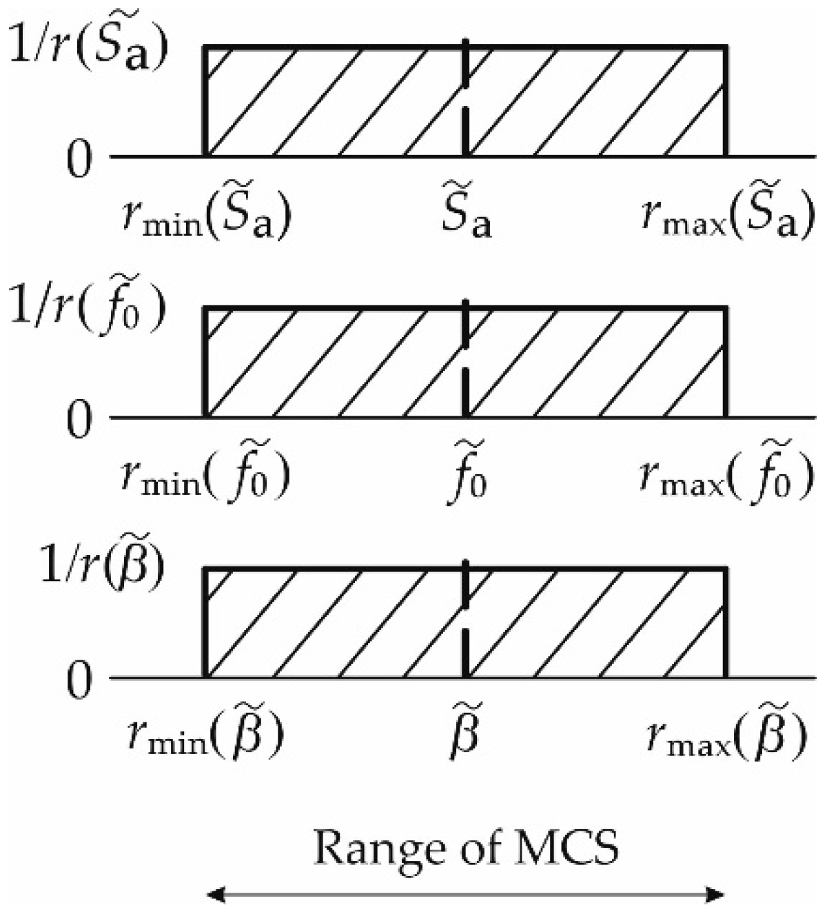should be determined. This can be carried out for the rectangular ranges shown in Figure 4 (the lines slanting to the right), by applying the MCP with the number of trials determined using Equation (3), where:

$$\begin{array}{c}{r}_{\min }\left(\alpha \right)=\alpha -u\left(\alpha \right)\\ r_{\max }\left(\alpha \right)=\alpha +u\left(\alpha \right)\\ r\left(\alpha \right)=r_{\max }\left(\alpha \right)-r_{\min }\left(\alpha \right)\end{array}$$

(21)

and $\alpha$ corresponds to the estimates ${\tilde{S}}_{\mathrm{a}}$, ${\tilde{f}}_0$, and $\widetilde{\beta ,}$ respectively, in the case of three ranges shown in Figure 4.

The trials of the MCP executed in three ranges were carried out by employing a uniform distribution. Hence, it is recommended to use the Wichmann–Hill pseudo-random number generator [28], according to the guidelines included in the JCGM supplement 1 [13]. The horizontal ranges of a uniform distribution in Figure 4 are constrained by the values of uncertainty associated with the parameter estimates of the accelerometer, while the vertical ranges of this distribution are contained in the range $\langle 0, \gamma \rangle ,$ where $\gamma =1/r\left(\alpha \right)$ is inversely proportional to the range of the parameter estimate variability.

Figure 5 shows the block diagram of the MCP for determining the $E^{\max }\left(y\right)$. This procedure includes three main sub-blocks:

• Back-to-back procedure for identification and determination of the accelerometer parameters and associated uncertainties.
• Selection of the special filter which is the reference for calculation of the energy at the output of accelerometer.
• Execution of the FPA.

The input parameter for the MCP is the number of MCts assumed in advance according to Equation (3), while the input parameters for the FPA are: number of iterations $J,$ value of time $T,$ quantization step size ${\Delta }_{\mathrm{s}}$ of the calculation, values of the signal limit $a,$ and initial Lagrange multiplier ${\xi }^0$.

5. Results

The results of testing the accelerometer of the type DJB A/1800/V are presented below. Typical parameters for the accelerometer, taken from the corresponding datasheet [29], are as follows:

–

voltage sensitivity $S_{\mathrm{a}}$ (±10%): 1.02 V/(m/s²),

–

frequency response (accelerometer bandwidth): 0.2 Hz–1 kHz ±5%,

–

maximum continuous g level: 4903 m/s²,

–

resonant frequency: $\approx$ 4 kHz.

The B&K8305 charge mode accelerometer was applied as the reference. The parameters of this accelerometer, contained in the datasheet [31], are:

–

charge sensitivity (±10%): 1.08 pC/g,

–

amplitude (±10%) and phase (±1°) range: 0.2 Hz–1 kHz.

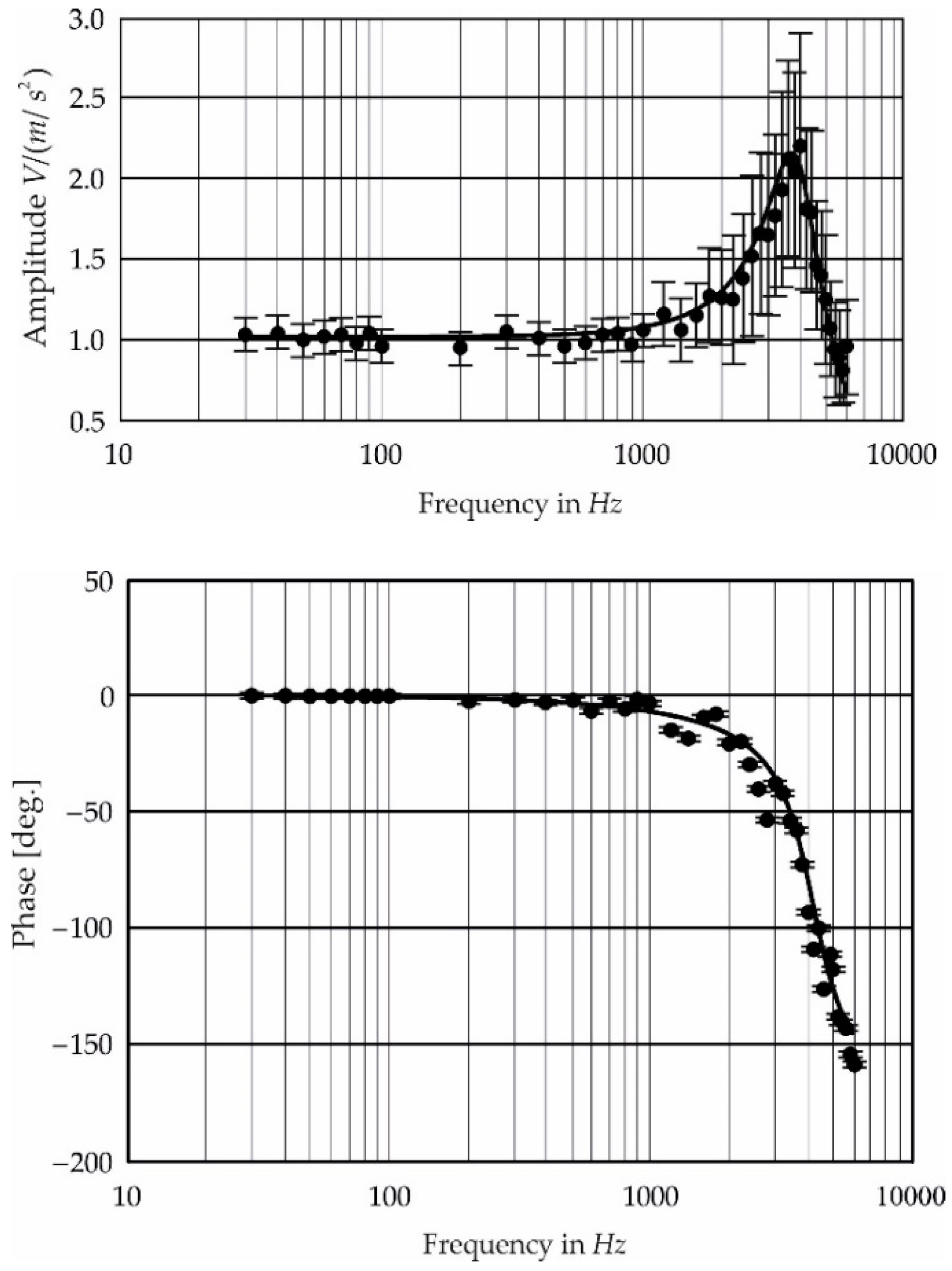
The results of the back-to-back identification are obtained based on the measurement of the amplitude and phase responses carried out for 42 frequencies within the range 30 Hz–6 kHz. This range was selected in such a way as to exceed the value of the resonant frequency since it has a significant influence on the value of the estimates ${\tilde{f}}_0$ and $\tilde{\beta }$.

The measurement points of both frequency responses, obtained for the above frequencies (the first column denoted by F), are contained in the second and third columns (denoted by A and $\mathit{\Phi }$) of

Table 1. Measurement points of the frequency responses together with expanded uncertainties (k = 2) for the accelerometer DJB A/1800/V.

F [Hz]	A [V/(m/s2)]	$\mathit{\Phi }$ [deg.]	u(A) [V/(m/s2)]	$u\left(\Phi \right)$ [deg.]	F [Hz]	A [V/(m/s2)]	$\mathit{\Phi }$ [deg.]	u(A) [V/(m/s2)]	$u\left(\Phi \right)$ [deg.]
30	1.03	−0.1	0.01	1.0	2000	1.26	−20.4	0.03	1.0
40	1.04	−0.4	0.01	1.0	2200	1.25	−19.5	0.04	1.0
50	1.00	−0.3	0.01	1.0	2400	1.38	−30.0	0.04	1.0
60	1.02	−0.5	0.01	1.0	2600	1.52	−40.5	0.05	1.0
70	1.03	−0.4	0.01	1.0	2800	1.66	−53.7	0.05	1.0
80	0.98	−0.7	0.01	1.0	3000	1.65	−38.1	0.05	1.0
90	1.04	−0.7	0.01	1.0	3200	1.77	−41.6	0.05	1.0
100	0.96	−0.9	0.01	1.0	3400	1.93	−53.8	0.06	1.0
200	0.95	−2.3	0.01	1.0	3600	2.12	−58.2	0.06	1.0
300	1.05	−2.0	0.01	1.0	3800	2.05	−73.1	0.06	1.0
400	1.01	−3.2	0.01	1.0	4000	2.20	−93.2	0.07	1.0
500	0.96	−2.4	0.01	1.0	4200	1.81	−108.9	0.05	1.0
600	0.98	−6.3	0.01	1.0	4400	1.79	−99.9	0.05	1.0
700	1.03	−3.0	0.01	1.0	4600	1.46	−126.2	0.04	1.0
800	1.04	−6.0	0.01	1.0	4800	1.40	−111.2	0.04	1.0
900	0.97	−2.4	0.01	1.0	5000	1.25	−117.6	0.04	1.0
1000	1.05	−3.5	0.01	1.0	5200	1.07	−138.0	0.03	1.0
1200	1.16	−14.9	0.02	1.0	5400	0.94	−140.0	0.03	1.0
1400	1.06	−18.7	0.02	1.0	5600	0.89	−143.0	0.03	1.0
1600	1.15	−9.6	0.02	1.0	5800	0.81	−154.4	0.02	1.0
1800	1.27	−8.2	0.03	1.0	6000	0.96	−158.5	0.03	1.0

.

The measurement points above are registered by the NI-6221 data acquisition card with a sampling rate equal to 100 kS/s and the computer programs developed in the LabVIEW software.

The expanded uncertainties u(A) and u($\mathit{\Phi }$) which are contained in the fourth and fifth columns of Table 1 were determined based on Table 1 included in the ISO 16063-21:2003(E) standard (7). These uncertainties are valid for the coverage factor $k=2$.

The accelerometer model responses (solid lines) obtained by utilizing the WLSP are shown in Figure 6. The covariance matrices involved in the basis kernel of the WLSP used for calculating the estimates of the accelerometer model parameters and applied for determining the uncertainties associated with these estimates are determined by using the MCP. The number $M$ of MCts, which is equal to $2\times {10}^5,$ was taken as the minimum acceptable value obtained based on Equation (3). The coverage probability $p$ equal to 0.95 was assumed in advance.

The expanded uncertainties, u(A) and u($\mathit{\Phi }$), are marked in Figure 6 by the solid vertical lines within the measurement points of both responses. The graphs of both responses are presented by using a logarithmic scale due to the wide range of considered frequencies.

The estimates ${\tilde{S}}_{\mathrm{a}}$, ${\tilde{f}}_0,$ and $\tilde{\beta }$ of the parameters of the accelerometer model and the associated uncertainties $u\left({\tilde{S}}_{\mathrm{a}}\right)$, $u\left({\tilde{f}}_0\right),$ and $u\left(\tilde{\beta }\right)$ determined by using the WLSP are tabulated in

Table 2. Estimated parameters and associated uncertainties obtained by using the weighted least squares procedure (WLSP).

${\tilde{\mathit{S}}}_{\mathit{a}}$ [V/(m/s2)]	${\tilde{\mathit{f}}}_0$ [Hz]	$\tilde{\mathit{\beta }}$ [–]	$\mathit{u}\left({\tilde{\mathit{S}}}_{\mathit{a}}\right)$ [V/(m/s2)]	$\mathit{u}\left({\tilde{\mathit{f}}}_0\right)$ [Hz]	$\mathit{u}\left(\tilde{\mathit{\beta }}\right)$ [–]
1.037	4073	0.3182	0.003	6	0.0004

.

The model responses shown in Figure 6 are obtained by relative approximation by using the functions $A\left(f\right)$ and $\phi \left(f\right)$ for the parameters tabulated in Table 2, where

$$A\left(f\right)=\frac{{\tilde{S}}_{\mathrm{a}}}{\sqrt{{\left[1-{\left(f/{\tilde{f}}_0\right)}^2\right]}^2+4{\tilde{\beta }}^2{\left(f/{\tilde{f}}_0\right)}^2}}$$

(22)

and

$$\phi \left(f\right)=-\arctan \frac{2\tilde{\beta }\left(f/{\tilde{f}}_0\right)}{1-{\left(f/{\tilde{f}}_0\right)}^2}$$

(23)

The estimates and associated uncertainties from Table 2 were utilized to determine the parameters ${\tilde{S}}_{\mathrm{a}}^{\max }$, ${\tilde{f}}_0^{\max },$ and ${\tilde{\beta }}^{\max }$ giving the maximum value of the reference energy determined by the FPA controlled by the MCP. 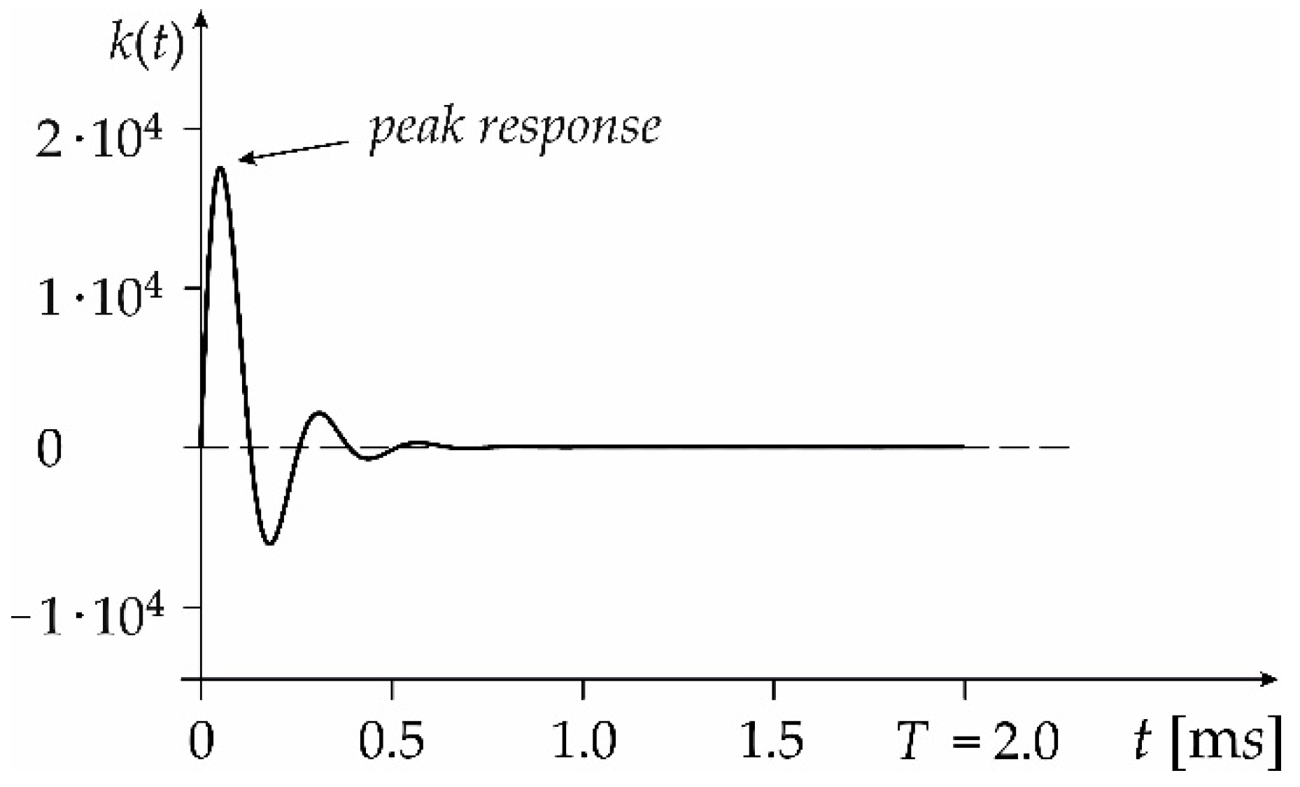The input parameters for the FPA were selected as: $J$ = 30, $T$ = 2 ms, ${\Delta }_{\mathrm{s}}$ = 2 μs, and ${\xi }^0$ = 1, and the value of signal limit $a$ = 1.037 V was assumed as equal to the estimate of the voltage sensitivity ${\tilde{S}}_{\mathrm{a}}$ of the considered accelerometer. The time $T$ was obtained from the steady state of the impulse response $k\left(t\right)$ calculated based on Equation (14). This steady state was assumed to be equal to 5% of the maximum deviation (peak response) from zero of this impulse response. The tenth-order ($L$ = 10) analog Butterworth filter was adopted and is described by Equation (6). The filter cut-off frequency $f_{\mathrm{c}}$ is equal to the frequency response of the considered accelerometer and is 1 kHz. The values of both the gain factor $a$ and the signal limit $a$ are equal to 1.03 V (i.e., the value of the estimate ${\tilde{S}}_{\mathrm{a}}$ of the accelerometer voltage sensitivity). The upper limit of the filter order results from the computational limitation of the MathCad program which was applied for calculation of the impulse response in the way of determining the inverse Laplace transform on the basis of the relevant transfer function $K_{\mathrm{f}}\left(s\right)$.

Figure 7 shows the impulse responses $k\left(t\right)$, where the maximum deviations of these responses from the steady state value are equal to 1764. The number of MCts for the procedure controlling the FPA was $2\times {10}^5,$ similar to the WLSP. Based on parameters and uncertainties given in Table 2, the following values were obtained: $u_{\min }\left({\tilde{S}}_{\mathrm{a}}\right)$ = 1.034 V/(m/s²); $u_{\max }\left({\tilde{S}}_{\mathrm{a}}\right)$ = 1.040 V/(m/s²); $u\left({\tilde{S}}_{\mathrm{a}}\right)$ = 0.016 V/(m/s²); $u_{\min }\left({\tilde{f}}_0\right)$ = 4067 Hz; $u_{\max }\left({\tilde{f}}_0\right)$ = 4079 Hz; $u\left({\tilde{f}}_0\right)$ = 12 Hz; $u_{\min }\left(\tilde{\beta }\right)$ = 0.3178; $u_{\max }\left(\tilde{\beta }\right)$ = 0.3186; and $u\left(\tilde{\beta }\right)$ = 8 for the ranges shown in Figure 4.

The values of the parameters ${\tilde{S}}_{\mathrm{a}}^{\max }$ = 1.038 V/(m/s²), ${\tilde{f}}_0^{\max }$ = 4070 Hz, and ${\tilde{\beta }}^{\max }$ = 0.3178, which give the maximum reference energy $E{\left(y\right)}^{\max }$ = 5.862 mV·m², are obtained by applying the MCP for $T$ = 2 ms, $m$ = 127,548, and $J$ = 15. The obtained uncertainty $u(E^{\max })$ of the MCP is equal to 0.008 mV·m².

The relationship between the maximum reference energy $E^{\max }\left(y\right)$ and the time $T$ of the considered accelerometer is linear [5] for the steady state of the impulse response $k\left(t\right)$ (i.e., for $T$ > 2 ms). Thus, it is possible to determine the functional relationship between this energy and any time $T$ higher than 2 ms. Hence, the value of energy $E^{\max }\left(y\right)$ should be determined for any time higher than 2 ms, and then the relevant formula can be easily determined based on the linear regression. For example, if $T$ = 10 ms, then we have $E^{\max }\left(y\right)$ = 34.115 mV·m² and $u(E^{\max })$ = 0.012 mV·m², which are obtained for $m$ = 93,515 and $J$ = 9. Based on the two values of the energy $E^{\max }\left(y\right)$ and the values of time $T,$ we have:

$$E{\left(y,T\right)}^{\max }=3531.0·T-1.2.$$

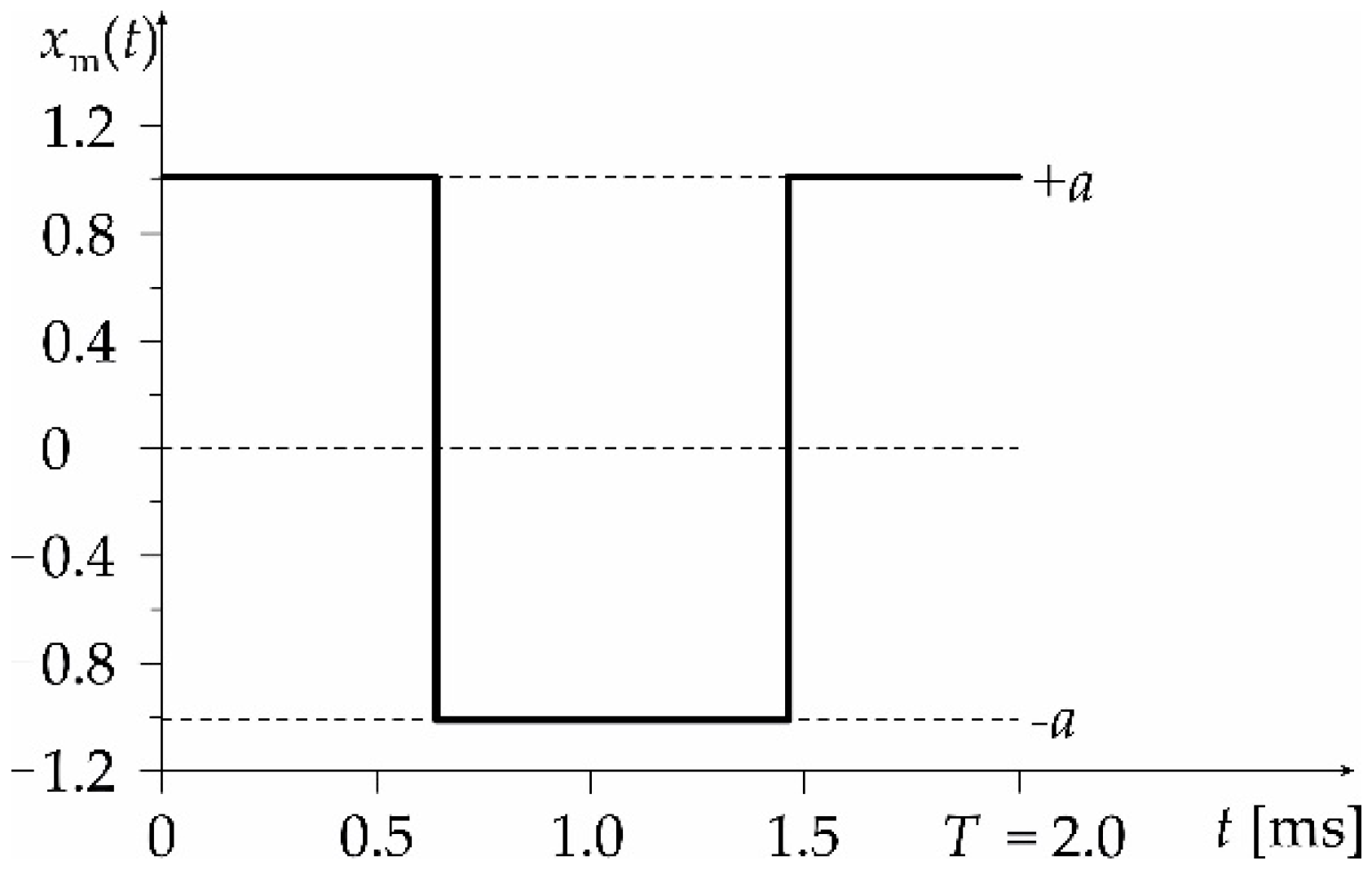
Figure 8 shows the signal $x_{\mathrm{m}}\left(t\right)$ with two reversals producing the $E^{\max }\left(y\right)$ at the output of the considered accelerometer obtained for $T$ = 2 ms.

The reversals of the signal $x_{\mathrm{m}}\left(t\right)$ are 0.68 ms and 1.49 ms.

6. Conclusions

The paper presents a proposal for the application of the FPA controlled by the MCP to determine the maximum reference energy at the output of accelerometers. Block diagrams together with a detailed description of the proposed solutions are presented.

The reference energy of the accelerometer should be understood as its output energy decreased by the output energy of the special filter (modeled by the low-pass type) with the cut-off frequency corresponding to the upper limit of the accelerometer frequency response. The lower limit of this response is neglected in this paper due to its low value (0.2 Hz).

Additionally, the MCP was used for parametric identification of both the parameters associated with the transfer function of the accelerometer and the associated uncertainties. Then, the value of the maximum reference energy was determined along with the associated uncertainties at the output of the accelerometer of the type DJB A/1800/V, considered as an example of the accelerometer. This was performed by checking the full range of the parameter variability of the accelerometer model by value-associated uncertainties. This is possible to perform only by using the MCP based on the pseudo-random number generator with a uniform distribution. This necessity results from the fact that the energy above can be obtained for the values of parameters contained within the variability ranges and not, for example, at their ends or in their middles. Only in this way it is possible to accurately determine the maximum reference energy, which can be the basis for mutual comparison of different types of accelerometers. The presentation of the relevant procedures together with a practical example giving the possibility of such comparison is the main contribution of this paper.