Properties of Fractional-Order Magnetic Coupling

Abstract

This paper presents the properties of fractional-order magnetic coupling. The difficulties connected with the analysis of two coils in dynamic states, resulting from the classical approach, provided motivation for studying the properties of fractional-order magnetic coupling. These difficulties arise from failure to comply with the commutation laws, i.e., a sudden power disappearance in the primary winding caused by a switch-mode power supply. Theoretically, under ideal conditions, a sudden power disappearance in the coil is, according to the classical method, manifested by a sudden voltage surge in the form of the Dirac delta function. As is well-known, it is difficult to obtain such ideal conditions in practice; the time of current disappearance does not equal zero due to the circuit breaker’s imperfection (even when electronic circuit breakers are used, the time equals several hundred nanoseconds). Furthermore, it is necessary to take into account phenomena occurring in real inductances, such as the skin effect, the influence of the ferromagnetic core and many other factors. It would be very difficult to model all these phenomena using classical differential calculus. The application of fractional-order differential calculus makes it possible to model them in a simple way by appropriate selection of coefficients and fractional-order derivatives. It should be mentioned that the analysis could be used, for example, in the case of high-voltage generation systems, including spark ignition systems of internal combustion engines. The use of fractional-order differential calculus will allow for more accurate modeling of phenomena occurring in such systems.

1. Introduction

The classical (standard) approach to the analysis and modeling of electrical systems usually ignores the effects of the non-ideality of elements and allows one to obtain a mathematical model based on integer-order differential equations. The use of this approach does not always lead to precise models. The application of fractional-order derivatives makes it possible to “compensate” for the missed phenomena. Real elements are characterized by loss, dielectric relaxation, electrochemical processes, magnetic heterogeneity, non-linearities, or simply operating conditions, e.g., temperature.

Classical differential and integral calculus is a well-studied area of mathematics, and its application can be found in numerous publications on the analysis of differentiation and integration, solving ordinary and partial differential equations, integral equations, etc. If fractional orders, e.g., 0.5, 1.8, or π, for derivatives and integrals are considered, we deal with differential-integral calculus of non-integer or fractional order. As it turns out, differential-integral calculus of fractional order can also be used with integer orders [1,2,3]. Derivatives of fractional order, also called differintegrals, are an interesting generalization of well-known dynamic systems, described by "classical" differential equations with derivatives of integer orders.

The use of fractional calculus in theoretical electrical engineering and circuit theory has enjoyed growing interest for several years. The appearance of entirely new electrotechnical components and devices, namely, supercapacitors, memory resistors called "memristors" [4,5,6], inductors with a skin effect [7], and coils with fractional mutual inductance [8], has been a reason for introducing C_α and L_β elements, which are described by differential-integral calculus of fractional order as a generalization of classical elements [9,10,11,12,13,14]. Descriptions employing differential calculus of fractional order have been extended to include phenomena occurring in real inductances. This comprises real coils (loss coils) with the skin effect, especially those with soft ferromagnetic cores, or containing electronic active systems, e.g., a generalized impedance converter (GIC) [15] and a coil with a fractional mutual inductance [16]. Other applications of fractional-order elements for materials and solutions described by chemical reactions are presented in [17,18].

The difficulties connected with the analysis of two coils in dynamic states, resulting from the classical approach, provided motivation for studying the properties of fractional-order magnetic coupling. It should be mentioned that the analysis can be used, for example, in the case of high-voltage generation systems, including spark ignition systems of internal combustion engines. The use of fractional-order differential calculus will allow for more accurate modeling of phenomena occurring in such circuits.

The paper is organized as follows. In the Introduction the problem is discussed, and Section 2 deals with the analysis of classical magnetic coupling of two coils and the response of such a system to voltage forcing in the form of a rectangular pulse. The next section contains a synthetic presentation of the mathematical apparatus used in the analysis. The definitions of selected derivatives of fractional order and their Laplace transformations are presented. The basic methods used to determine the inverse Laplace transform of fractional-order systems allow the approximation of the s^α factor by the quotient of polynomials with integer powers. The main part of the paper is covered by Section 4, presenting the analysis of fractional-order magnetic coupling of two coils. This section includes the results of theoretical analysis supported by the results of digital simulations. It can be concluded that open-core ferromagnetic coils, which are non-linear elements with ambiguous characteristics, can be more realistically modeled using fractional-order calculus. Experimental tests on a real object (an ignition coil), confirming the purposefulness of the analysis, are presented in Section 5.

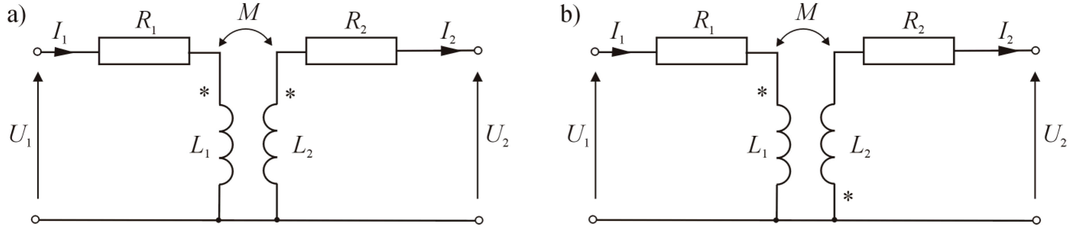
2. The Classic Magnetic Coupling of Two Coils

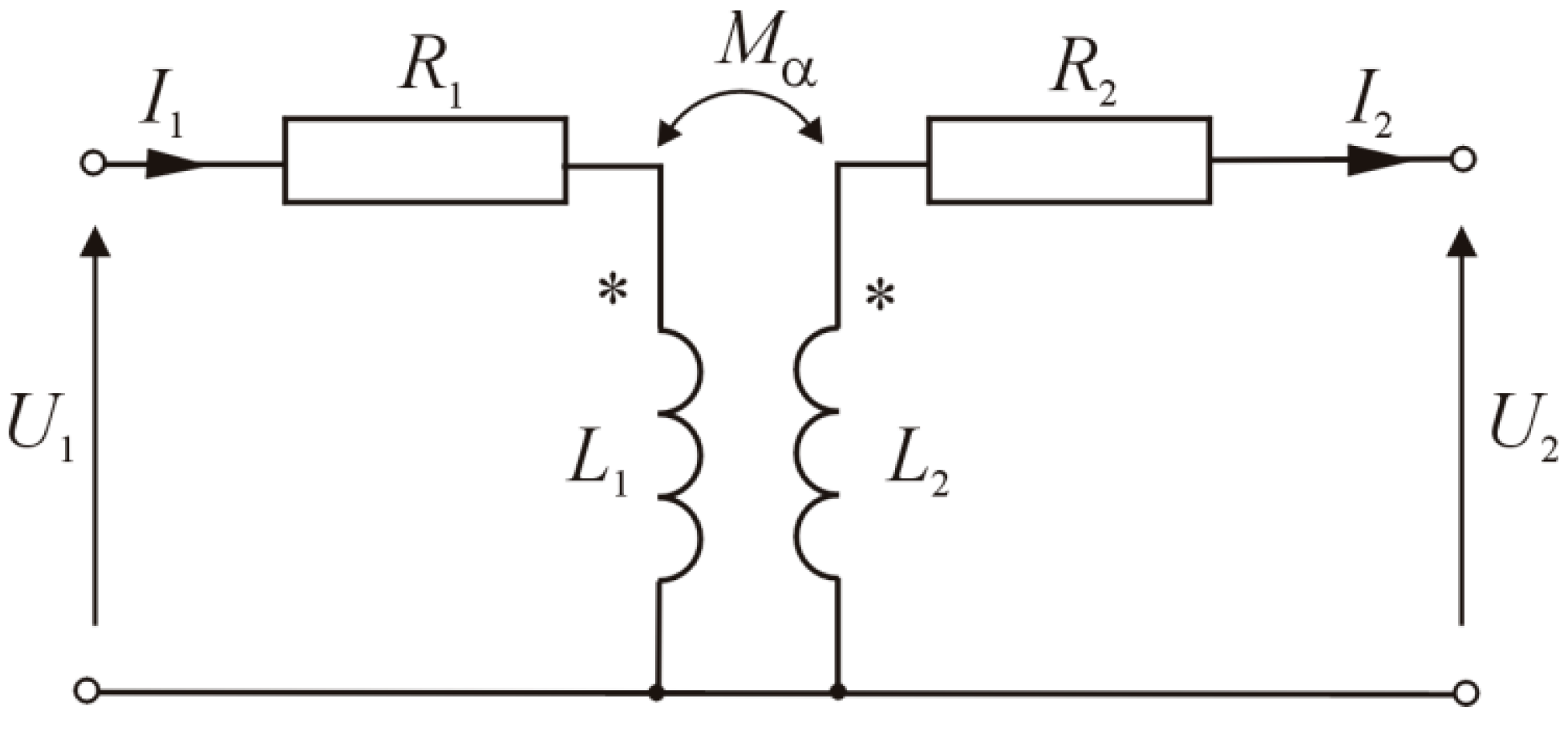
To compare the magnetic couplings of two coils with matching and opposite magnetic polarity, generally known relationships for classical magnetic coupling are presented. The object studied is the electrical circuit of two coils shown in Figure 1.

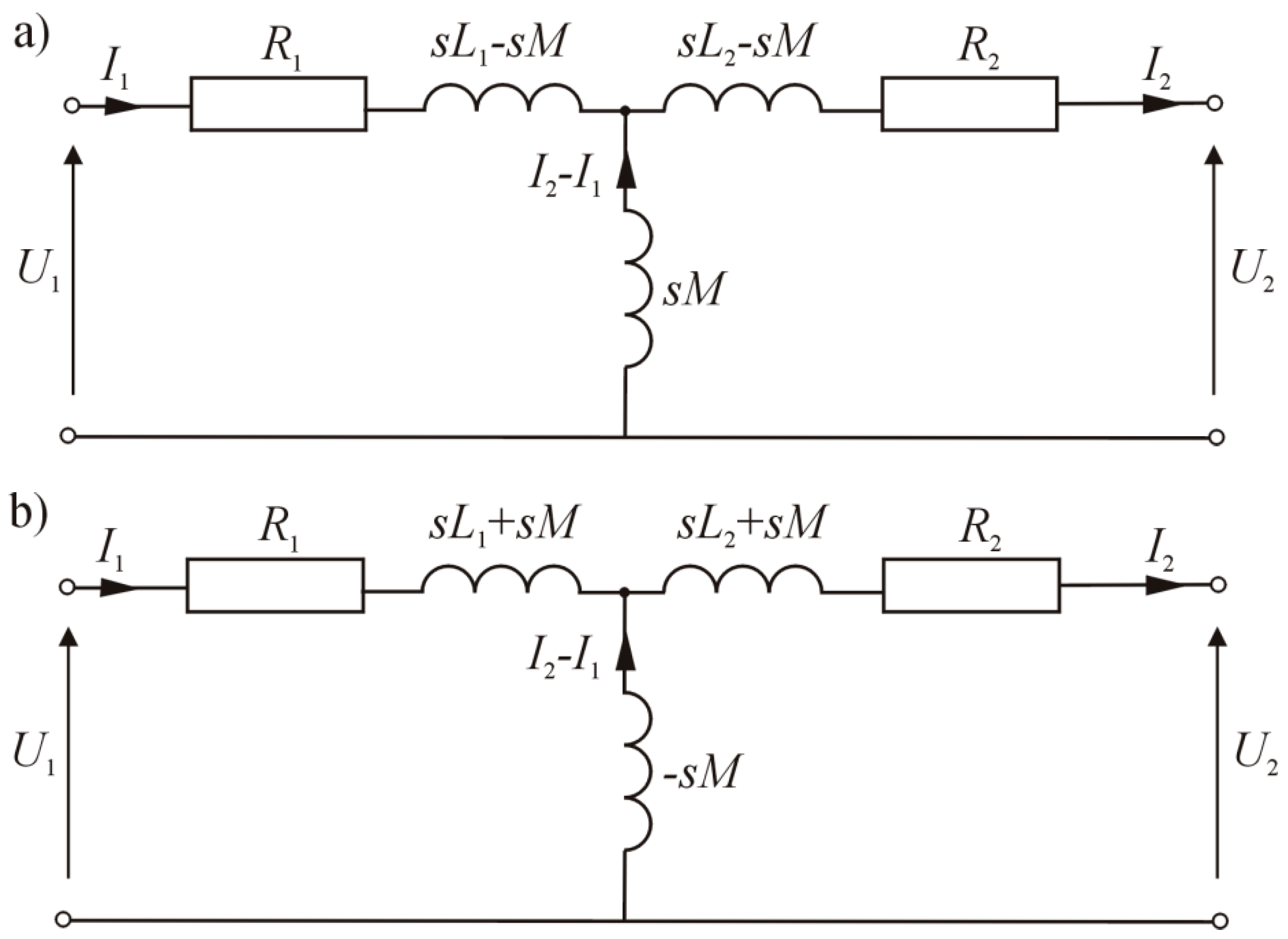
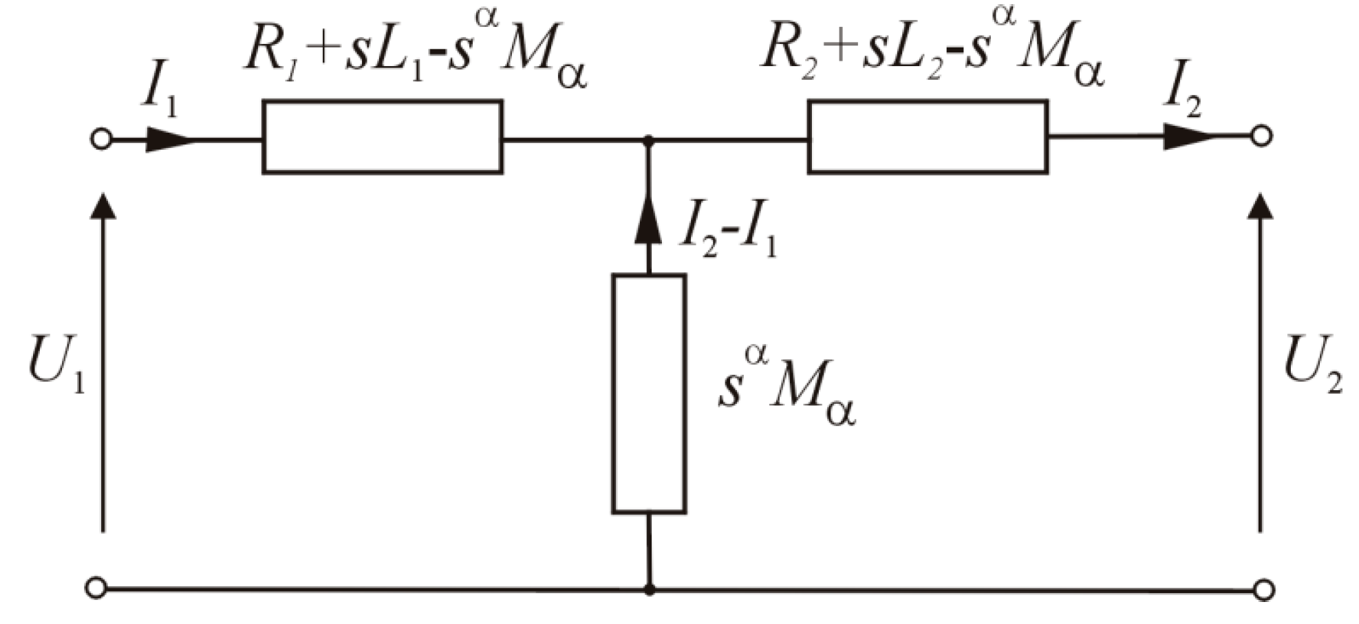
As we know, by eliminating coupling and using the Laplace transform, it is possible to obtain the diagrams of circuits shown in Figure 2.

If the systems in Figure 2 are considered to be two-port networks of T type, the following chain matrix can be determined:

$$A_T=\left[\begin{array}{cc}1+Z_{1}Y& Z_1+Z_2+Z_1{Z}_{2}Y\\ Y& 1+Z_{2}Y\end{array}\right]$$

(1)

Therefore, for the two-port networks in Figure 2a,b, the matrix has the form:

$$A_a=\left[\begin{array}{cc}1+\frac{R_1+s\left(L_1-M\right)}{sM}& R_1+s\left(L_1-M\right)+R_2+s\left(L_2-M\right)+\frac{\left[R_1+s\left(L_1-M\right)\right]\left[R_2+s\left(L_2-M\right)\right]}{sM}\\ \frac{1}{sM}& 1+\frac{R_2+s\left(L_2-M\right)}{sM}\end{array}\right]$$

(2)

$$A_b=\left[\begin{array}{cc}1+\frac{R_1+s\left(L_1+M\right)}{-sM}& R_1+s\left(L_1+M\right)+R_2+s\left(L_2+M\right)+\frac{\left[R_1+s\left(L_1+M\right)\right]\left[R_2+s\left(L_2+M\right)\right]}{-sM}\\ \frac{1}{-sM}& 1+\frac{R_2+s\left(L_2-M\right)}{-sM}\end{array}\right]$$

(3)

Assuming that two-port networks are in idle state, the following equation applies:

$$\left[\begin{array}{l}{U}_{10}\\ I_{10}\end{array}\right]\left[\begin{array}{l}{A}_{11}{A}_{12}\\ A_{21}{A}_{22}\end{array}\right]\left[\begin{array}{l}{U}_{20}\\ 0\end{array}\right]$$

(4)

Thus,

$$U_{20}=\frac{U_{10}}{A_{11}},I_{10}=\frac{A_{21}}{A_{11}}{U}_{10}$$

(5)

Considering the relations in (2), one obtains:

$$U_{20}=\frac{U_{10}sM}{\left(R_1+s{L}_1\right)}\mathrm{and}:I_{10}=\frac{U_{10}}{s\left(R_1+s{L}_1\right)}$$

(6)

Analyzing the relations, in the context of the elements of the matrices A_a and A_b, it is easy to conclude that the output voltage and the input current of two-port networks a) and b) will differ only by sign.

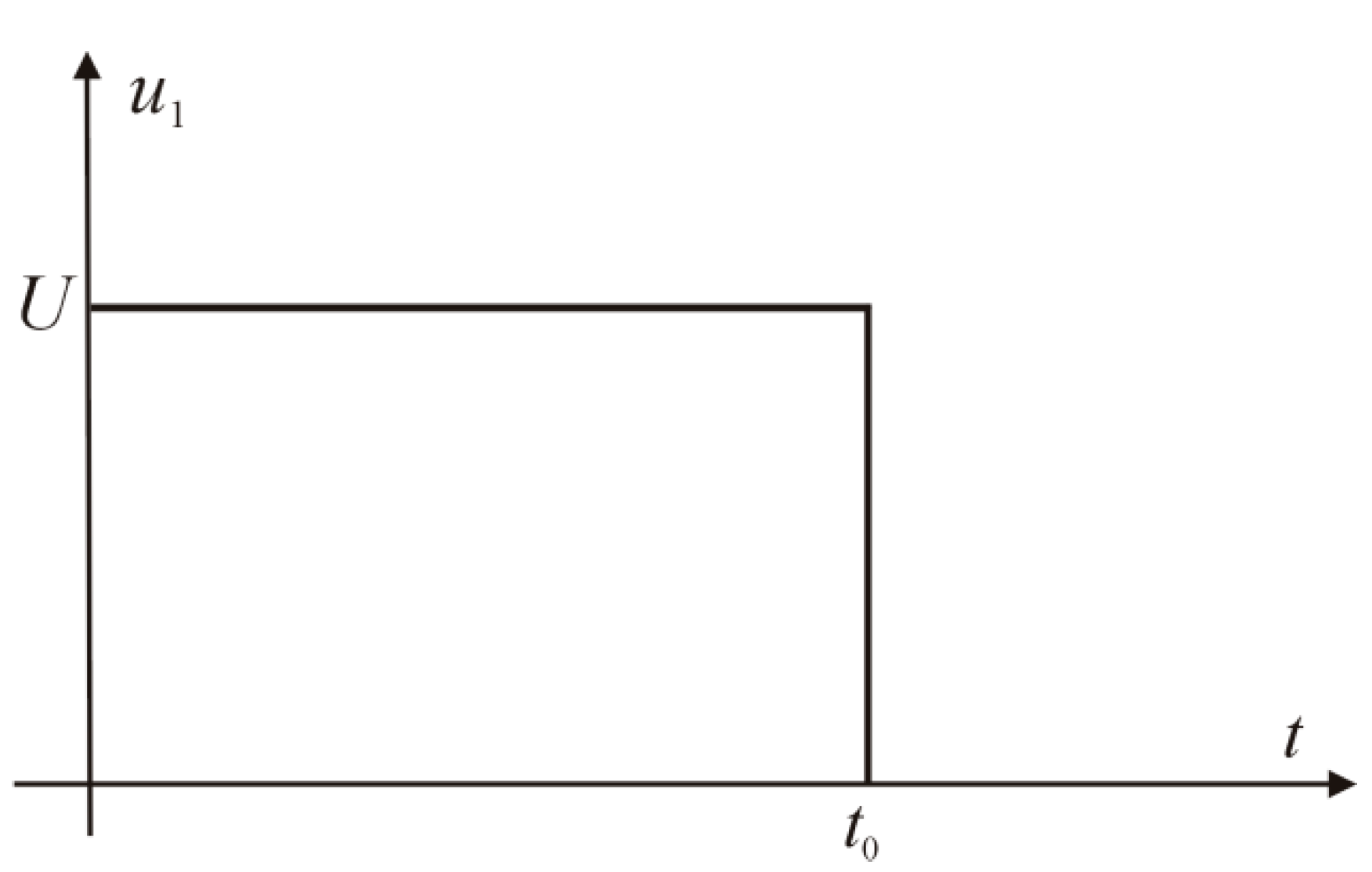
For the voltage forcing in the form of a rectangular pulse (Figure 3), voltage u₁₀(t) is:

$$u_{10}\left(t\right)=U\left[1\left(t\right)-1\left(t-t_0\right)\right]$$

(7)

where U: supply voltage; t₀: pulse duration; 1(t): unit function.

The voltage transform is written out as:

$$U_{10}\left(s\right)=\frac{U}{s}\left(1-e^{-s{t}_0}\right)$$

(8)

Thus, the voltage transform at the output and the current transform at the two-terminal input are expressed by the relations:

$$U_{20}=\frac{MU\left(1-e^{-s{t}_0}\right)}{\left(R_1+s{L}_1\right)},$$

(9)

$$I_{10}=\frac{U\left(1-e^{-s{t}_0}\right)}{s\left(R_1+s{L}_1\right)}$$

(10)

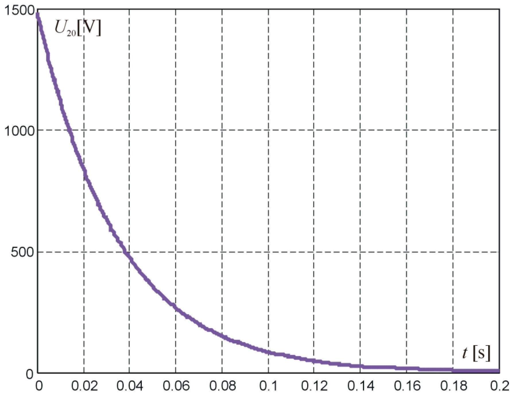
By calculating the inverse transform for time $t$ < $t_0$, the system response to rectangular-pulse forcing was obtained. The voltage at the output and current at the input of the two-port network are shown in Figure 4 and Figure 5.

The waveforms were obtained for the real parameters of ignition coils, that is R₁ = 0.2 Ω; L₁ = 7 mH; R₂ = 1380 Ω; L₂ = 40 mH; U = 13 V [19,20,21,22].

When considering the system response to the forcing assumed for time $t\ge t_0$, the initial condition should be taken into account—i.e., currents passing through coils at $t=t_0$. Then, when analyzing the circuits in Figure 2a or Figure 2b, it turns out that only the current passing through the L₁ coil should be taken into account, since I₂ = 0. Hence, for the case of Figure 2a, the diagram shown in Figure 6 was obtained.

.

By calculating the voltage component at the two-terminal output, one obtains:

$$U_{20}=-\frac{MU{e}^{-s{t}_0}}{\left(R_1+s{L}_1\right)}+\frac{L_1{I}_1\left(t_0\right)sM}{\left(R_1+s{L}_1\right)}$$

(11)

By determining the inverse transform of the first component of Equation (11), one obtains the waveforms that are the same as those shown in Figure 4 and Figure 5, but shifted in time by t₀ and inverse. The transform of the second component, resulting from the initial condition (it was assumed that $I_1\left(t_0\right)=\frac{U}{R_1}$), can be written as:

$$U_{202}=\frac{sMU{L}_1}{R_1\left(R_1+s{L}_1\right)}=\frac{MU{L}_1}{L_1{R}_1}-\frac{MUL}{\left(R_1+s{L}_1\right)}$$

(12)

As can be seen, one of the components on the right-hand side of Equation (12) is constant, i.e., independent of s, which means that its inverse transform will be the Dirac delta shifted in time by t₀.

$${\mathcal{L}}^{-1}\left\{\frac{MU{L}_1}{L_1{R}_1}\right\}=\frac{MU{L}_1}{L_1{R}_1}\delta \left(t-t_0\right)$$

(13)

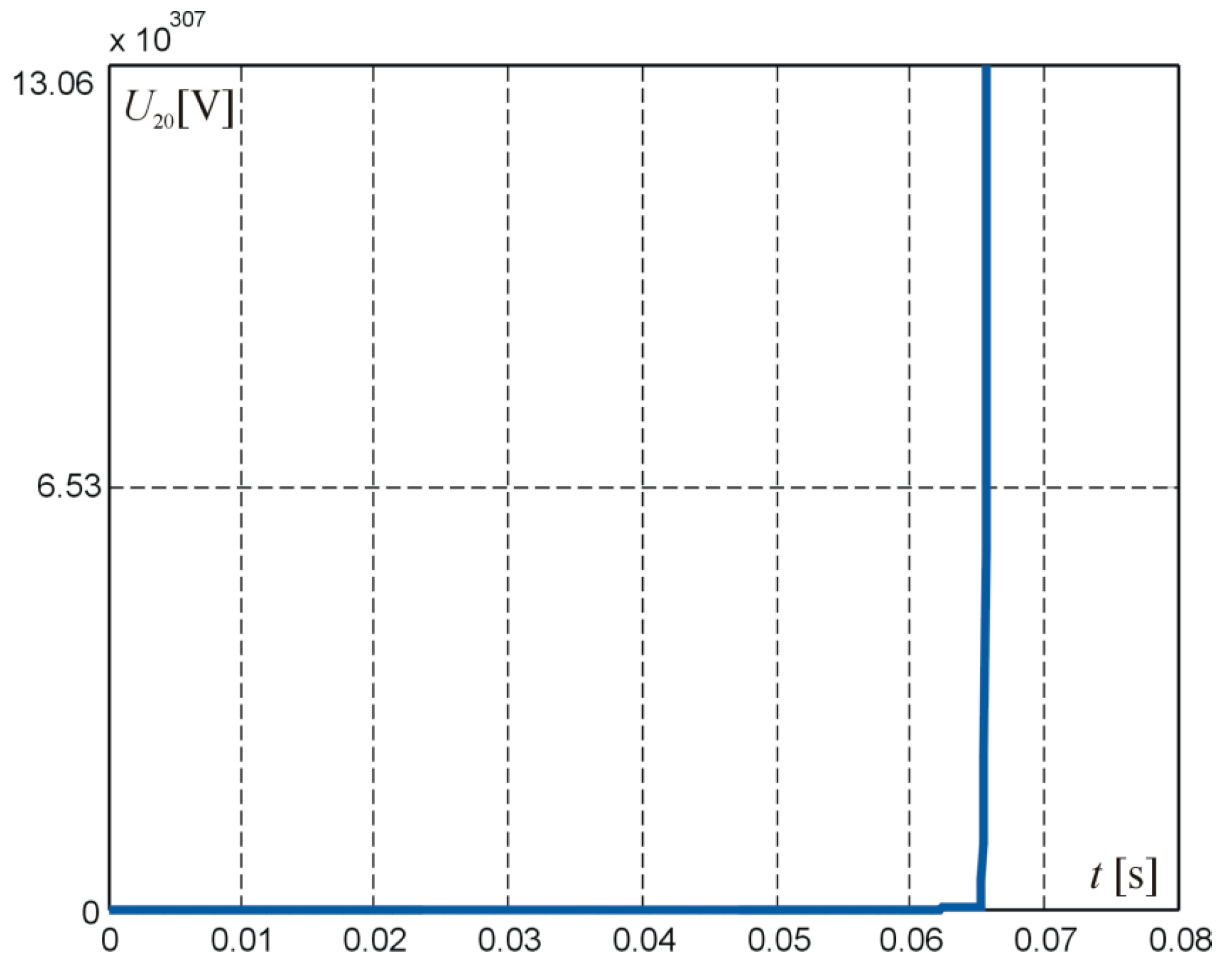
The result of the digital simulation of the solution is shown in Figure 7.

An electrical circuit with such forcing cannot be considered a classical one because the condition of current continuity in the coil is not met. Therefore, fractional-order calculus should be used to analyze it. Selected elements of the mathematical apparatus used in fractional-order calculus are presented in the next section.

3. Selected Elements of Fractional-Order Calculus

This section presents definitions of fractional-order derivatives in the Caputo and Riemann–Liouville senses, and the corresponding Laplace transforms. The approximation methods used to determine the inverse Laplace transform of fractional-order systems of equations, including the continued fraction expansion (CFE) and Oustaloup methods, are discussed.

3.1. Definitions of Fractional-Order Derivatives

There are many definitions of fractional-order integrals and derivatives. One of them is the Riemann–Liouville differintegral. Only the integral on the left-hand side, mainly used in engineering applications, is applied by the authors. The definition of derivative is obtained from the definition of the Riemann–Liouville fractional integral, which is a generalization of the formula for the n-th-order integral, and is also based on a well-known formula of classical differential calculus, namely:

$$\frac{d^n}{d{x}^n}f(x)=\frac{d^k}{d{x}^k}{I}_{}^{k-n}f(x)$$

(14)

where function f(x) is n-times differentiable in the range [a, b]; k, n ∈ N; and k > n.

Definition 1.

The left-hand side Riemann–Liouville differintegral of the order α ∈ C, (Re{α} > 0) of the real function f(x) is defined as:

$${}_a{}^{RL}D{}_t^{\alpha }f(t)=\frac{d^k}{d{t}^k}{I}^{(k-\alpha )}f(t)=\frac{1}{\mathsf{\Gamma }(k-\alpha )}\frac{d^k}{d{t}^k}{\displaystyle \underset{a}{\overset{t}{\int }}{(t-\tau )}^{k-\alpha -1}}f(\tau )d\tau ,$$

(15)

where$k-1\le \alpha \le k,k\in N\cup \left\{0\right\}$.

Detailed descriptions of the Riemann–Liouville differintegral can be found, among others, in [3,23,24,25].

Introduced by Michael Caputo in 1967 in [26], the definition of the Riemann–Liouville fractional integral is also used. Comparison of the Riemann–Liouville derivative and Caputo’s (C) derivative shows that, in the latter, the order of integration and differentiation is inverse, namely:

$$\frac{d^n}{d{x}^n}f(x)=I_{}^{k-n}\frac{d^k}{d{x}^k}f(x)$$

(16)

This affects the final structure of the derivative defined as follows:

Definition 2.

In the Caputo sense, the derivative of the order$\alpha (\alpha \in {\mathit{R}}_{+})$is called the operator,

$$L\left\{f^n\left(t\right);s\right\}=s^{n}F\left(s\right)-{{\displaystyle \sum }}_{k=0}^{n-1}{s}^{n-k-1}{f}^{\left(k\right)}\left(0\right)=s^{n}F\left(s\right)-{{\displaystyle \sum }}_{k=0}^{n-1}{s}^k{f}^{\left(n+k+1\right)}\left(0\right),$$

(17)

where$k-1\le \alpha \le k$.

The definitions of the fractional-order derivatives are not equivalent in a general case. However, under certain assumptions, there are similarities between them, including the problems with interpretation of initial conditions.

An important feature of the Caputo derivative is that initial conditions include derivatives of integer order. Another difference between the Caputo and the Riemann–Liouville definitions is the derivative of the constant function. For the lower limit, $\alpha =-\infty$, the Caputo and Riemann–Liouville definitions are equivalent.

3.2. The Laplace Transform of Fractional-Order Derivatives

The Laplace transform is frequently used to solve engineering problems. Its definition, similarly to that of a fractional derivative, is a generalization of concepts from classical calculus. The relations for the Laplace transform and its inverse are well-known and not discussed here. The Laplace transform of fractional-order derivatives can be calculated using the relations for the transform of the n-th-order classical derivative:

$$L\left\{f^n\left(t\right);s\right\}=s^{n}F\left(s\right)-{{\displaystyle \sum }}_{k=0}^{n-1}{s}^{n-k-1}{f}^{\left(k\right)}\left(0\right)=s^{n}F\left(s\right)-{{\displaystyle \sum }}_{k=0}^{n-1}{s}^k{f}^{\left(n+k+1\right)}\left(0\right),$$

(18)

Furthermore, for the fractional-order derivatives in the Riemann–Liouville sense,

$$L\left\{f\left(t\right)\times g\left(t\right);s\right\}=F\left(s\right)G\left(s\right),$$

(19)

The practical application of the transform is limited due to the lack of physical interpretation of the initial values of fractional derivatives for the lower limit t = 0. Likewise, a formula for a fractional derivative in the Caputo sense can be obtained:

$$L\left\{{}_0{}^{RL}D{}_x^{\alpha }f\left(t\right);s\right\}=s^{\alpha }F\left(s\right)-{{\displaystyle \sum }}_{k=0}^{n-1}{s}^k{\left[{}_0{}^{RL}D{}_x^{\alpha -k-1}f\left(t\right)\right]}_{t=0},n-1\le \alpha <n.$$

(20)

Its practical application is much wider because the initial conditions for t = 0 refer to derivatives of integer orders whose physical interpretations are well-known.

For derivatives of fractional order, the Laplace transform assuming zero initial conditions is:

$$L\left\{{}_0{}^{C}D{}_x^{\alpha }f\left(t\right);s\right\}=s^{\alpha }F\left(s\right)-{{\displaystyle \sum }}_{k=0}^{n-1}{s}^{\alpha -k-1}{f}^k\left(0\right),n-1\le \alpha <n.$$

(21)

where F(s) is the transform of the Laplace function f(t).

The detailed properties of the Laplace transform are presented in [3,27].

3.3. Selected Approximation Methods in the Analysis of Fractional-Order Electrical Circuits

The methods most commonly used to determine the inverse Laplace transform of fractional order circuits are those that allow the approximation of the s^α factor by the quotient of polynomials with integer powers s. Continued fraction expansion (CFE) is such a method. It consists of the expansion of the expression (1 + x), $0\le \alpha \le 1$ into an infinite continued fraction. By substituting x = s − 1 and taking into account successive terms, the s^α approximations of the required order and accuracy are obtained.

In the CFE method, the s^α factor can be presented as the quotient of the polynomials of the s variable and the order of the α derivative—here, these variables have integer powers [28,29].

$$s^{\alpha }\cong \frac{N\left(s,\alpha \right)}{D\left(s,\alpha \right)}=\frac{{\displaystyle \sum _{k=0}^A{P}_{Ak}\left(\alpha \right)s^{A-k}}}{{\displaystyle \sum _{k=0}^A{Q}_{Ak}\left(\alpha \right)s^{A-k}}}$$

(22)

where A: the order of approximation; P_Ak(α) and Q_Ak(α): α polynomials of A order.

It is shown in [30] that approximation of the order of A = 5 gives relatively the best accuracy for fifth-degree polynomials. The higher orders of approximation result in an increased number of components in polynomials and a slight improvement in accuracy. This means that higher orders of approximation cause, apart from an increased number of components in polynomials and, therefore, a greater number of poles and a more complex numerical implementation, a relatively minor change in the solution, which is interpreted as a slight improvement in accuracy. Thus,

$$s^{\alpha }=\frac{P_{50}{s}^5+P_{51}{s}^4+P_{52}{s}^3+P_{53}{s}^2+P_{54}s+P_{55}}{Q_{50}{s}^5+Q_{51}{s}^4+Q_{52}{s}^3+Q_{53}{s}^2+Q_{54}s+Q_{55}}$$

(23)

where:

$$\begin{array}{l}{P}_{50}=Q_{55}=-a^5-15a^4-85a^3-225a^2-274a-120\\ P_{55}=Q_{50}=a^5-15a^4+85a^3-225a^2+274a-120\\ P_{51}=Q_{54}=5a^5+45a^4+5a^3-1005a^2-3250a-3000\\ P_{54}=Q_{51}=-5a^5+45a^4-5a^3-1005a^2+3250a-3000\\ P_{52}=Q_{53}=-10a^5-30a^4+410a^3+1230a^2-4000a-12000\\ P_{52}=Q_{53}=10a^5-30a^4-410a^3+1230a^2+4000a-12000\end{array}$$

The second method used to approximate the s^α factor is the expansion into the Oustaloup series, where for frequency range (ω_l,ω_h), it is shown as transfer function H(s) [31,32,33,34]:

$$s^{\alpha }\approx H\left(s\right)=C_0{{\displaystyle \prod }}_{k=-N}^N\frac{s+{\omega }_k^{’}}{s+{\omega }_k}$$

(24)

where N: the order of approximation; C₀: the gain described by the following relation:

$$C_0={\left(\frac{{\omega }_h}{{\omega }_1}\right)}^{-\frac{\alpha }{2}}{{\displaystyle \prod }}_{k=-N}^N\frac{{\omega }_k}{{\omega }_k^{’}}$$

(25)

where ω^’_k: zeros and ω_k: the poles of the H(s) transfer function, which are:

$${\omega }_k^{’}={\omega }_l{\left(\frac{{\omega }_h}{{\omega }_1}\right)}^{\frac{k+N+0.5\left(1-\alpha \right)}{2N+1}}$$

(26)

$${\omega }_k={\omega }_l{\left(\frac{{\omega }_h}{{\omega }_1}\right)}^{\frac{k+N+0.5\left(1+\alpha \right)}{2N+1}}$$

(27)

Substituting (24) into (22), one obtains:

$$N\left(s,\alpha \right)=C_0{{\displaystyle \prod }}_{k=-N}^N\left(s+{\omega }_k^{’}\right),D\left(s,\alpha \right)={{\displaystyle \prod }}_{k=-N}^N\left(s+{\omega }_k\right)$$

(28)

It should be stressed that since the polynomials in the above approximations contain an integer of s, the inverse transform can be determined by standard methods [35,36].

4. Fractional-Order Magnetic Coupling of Two Coils

Figure 8 presents the electrical circuit with fractional-order magnetic coupling between two coils.

The following equations can be written out for the model:

$$\{\begin{array}{l}{u}_1=i_1{R}_1+L_1\frac{d{i}_1}{dt}-M_{\alpha }\frac{d^{\alpha }{i}_2}{d{t}^{\alpha }}\\ u_2+i_2{R}_2-M_{\alpha }\frac{d^{\alpha }{i}_1}{d{t}^{\alpha }}+L_2\frac{d{i}_2}{dt}=0\end{array}$$

(29)

after the Laplace transformation with zero initial conditions, one obtains:

$$\{\begin{array}{l}{U}_1(s)=I_1(s)R_1+s{L}_1{I}_1(s)-s^{\alpha }{M}_{\alpha }{I}_2(s)\\ U_2(s)+R_2{I}_2(s)-s^{\alpha }{M}_{\alpha }{I}_1(s)+s{L}_2{I}_2(s)=0\end{array}$$

(30)

After transformation, the equations assume the form:

$$\{\begin{array}{l}{U}_1(s)=I_1(s)R_1+s{L}_1{I}_1(s)-s^{\alpha }{M}_{\alpha }{I}_2(s)+s^{\alpha }{M}_{\alpha }{I}_1(s)-s^{\alpha }{M}_{\alpha }{I}_1(s)\\ U_2(s)+R_2{I}_2(s)-s^{\alpha }{M}_{\alpha }{I}_1(s)+s{L}_2{I}_2(s)+s^{\alpha }{M}_{\alpha }{I}_2(s)-s^{\alpha }{M}_{\alpha }{I}_2(s)=0\end{array}$$

(31)

After ordering, the following relation is obtained:

$$\{\begin{array}{l}{U}_1(s)=I_1(s)R_1+(s{L}_1-s^{\alpha }{M}_{\alpha })I_1(s)-s^{\alpha }{M}_{\alpha }[I_2(s)-I_1(s)]\\ U_2(s)+R_2{I}_2(s)+(s{L}_2-s^{\alpha }{M}_{\alpha })I_2(s)+s^{\alpha }{M}_{\alpha }[I_2(s)-I_1(s)]=0\end{array}$$

(32)

This system of equations corresponds to the electrical circuit in Figure 9.

It should be noted that in [8], the same system was obtained with the use of a different algorithm.

If we assume that the circuit in Figure 9 is a T-type two-port network, then on the basis of Equation (1), its chain matrix has the form:

$$A=\left[\begin{array}{cc}1+\frac{R_1+s{L}_1-s^{\alpha }M}{s^{\alpha }M}& R_1+s{L}_1-s^{\alpha }M+R_2+s{L}_2-s^{\alpha }M+\frac{\left(R_1+s{L}_1-s^{\alpha }M\right)\left(R_2+s{L}_2-s^{\alpha }M\right)}{s^{\alpha }M}\\ \frac{1}{s^{\alpha }M}& 1+\frac{R_2+s{L}_2-s^{\alpha }M}{s^{\alpha }M}\end{array}\right]$$

(33)

Following the same procedure as in the case of classical coupling, the relations determining output voltage and input current transforms at the input of the two-port network in Figure 9 take the form:

$$U_{20}=\frac{U_{10}{s}^{\alpha }M}{\left(R_1+s{L}_1\right)},\hspace{1em}{I}_{10}=\frac{U_{10}}{s\left(R_1+s{L}_1\right)}$$

(34)

Next, if the rectangular-pulse forcing shown in Figure 3 is considered, the relations are:

$$U_{20}=\frac{s^{\alpha }MU\left(1-e^{-s{t}_0}\right)}{s\left(R_1+s{L}_1\right)},\hspace{1em}{I}_{10}=\frac{U\left(1-e^{-s{t}_0}\right)}{s\left(R_1+s{L}_1\right)}$$

(35)

As can be seen, the expression for the current at the input of the two-port network has the same form as classical coupling.

After substituting the s^α factor by the quotient of polynomials according to the CFE method (22) or the Oustaloup series (24), the relation has the form:

$$U_{20}=\frac{\frac{N(s,\alpha )}{D(s,\alpha )}MU}{s\left(R_1+s{L}_1\right)}=\frac{N(s,\alpha )MU}{sD(s,\alpha )\left(R_1+s{L}_1\right)}$$

(36)

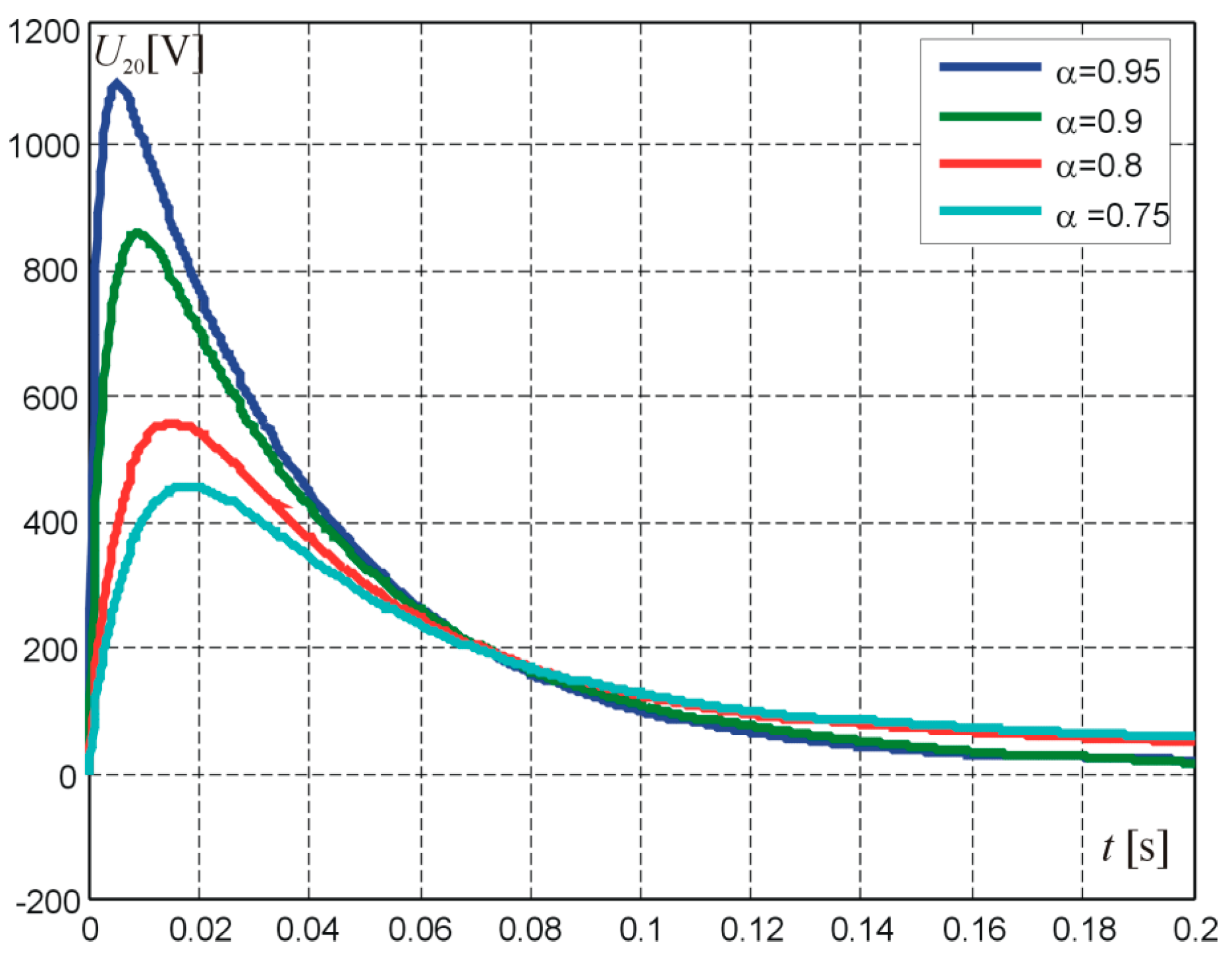
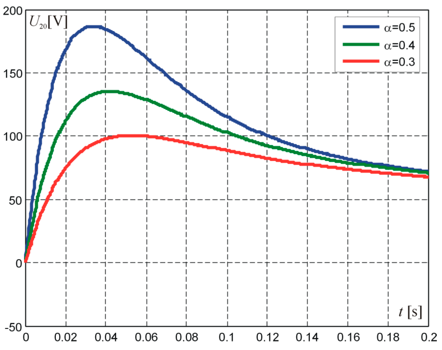
By calculating the inverse transform for the time $t$ < $t_0$, voltage curves at the output of a two-port network with rectangular-pulse forcing were obtained for α = 0.95, 0.9, 0.8, 0.75, as shown in Figure 10.

Figure 11 shows voltage curves for α = 0.5, 0.4, 0.3.

After considering the circuit response to rectangular-pulse forcing in time $t\ge t_0$ and taking into account the initial condition, i.e., the diagram presented in Figure 6, the following relations are written out:

$$U_{20}=\frac{-s^{\alpha }MU{e}^{-s{t}_0}}{s\left(R_1+s{L}_1\right)}+\frac{s^{\alpha }M{L}_1{I}_{10}}{\left(R_1+s{L}_1\right)},$$

(37)

$$I_{10}=\frac{-U{e}^{-s{t}_0}}{s\left(R_1+s{L}_1\right)}+\frac{L_1{I}_{10}}{\left(R_1+s{L}_1\right)}$$

(38)

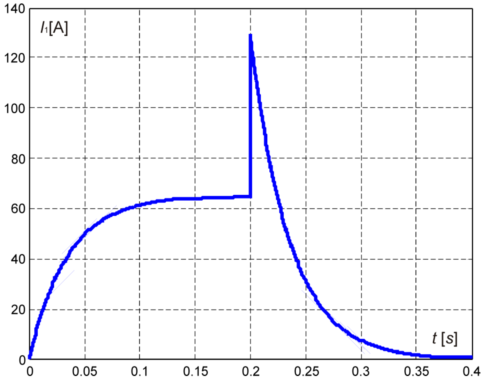
The expression determining the current at the input of the two-port network does not contain the s^α factor, so the reverse transform can be determined directly:

$$i_1=\frac{U}{R_1}-\frac{U}{R_1}{e}^{-\frac{R_1}{L_1}t}-\frac{U}{R_1}1(t-t_0)+\frac{U}{R_1}{e}^{-\frac{R_1}{L_1}t}1(t-t_0)+i_{10}(t_0)e^{-\frac{R_1}{L_1}t}1(t-t_0)$$

(39)

Figure 12 shows the current curve at the input of the two-port network for the whole time interval.

The voltage transform at the output of the two-port network is:

$$U_{20}=\frac{-N\left(s,\alpha \right)MU{e}^{-s{t}_0}}{sD\left(s,\alpha \right)\left(R_1+s{L}_1\right)}+\frac{N\left(s,\alpha \right)M{L}_1{I}_{10}}{D\left(s,\alpha \right)\left(R_1+s{L}_1\right)}$$

(40)

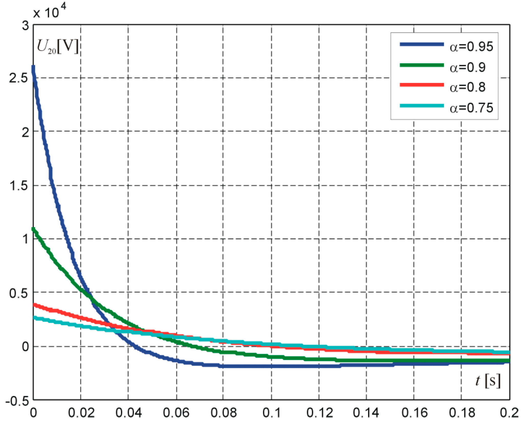
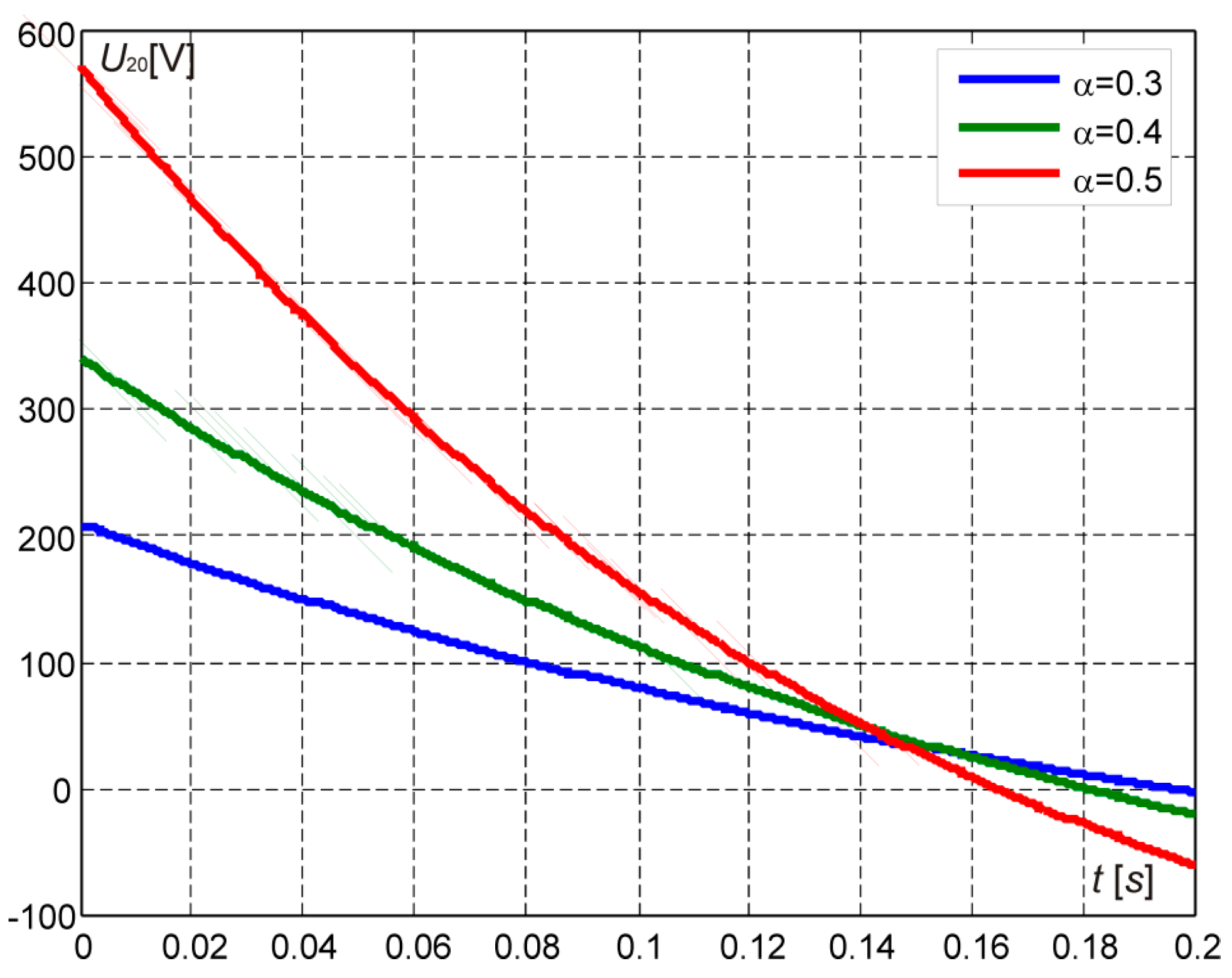
By calculating the inverse transform for the time $t\ge t_0$, voltage waveforms for the assumed forcing at the output of the two-port network are obtained. Figure 13 shows voltage curves for α = 0.95, 0.9, 0.8, 0.75, and Figure 14 for α = 0.5, 0.4, 0.3.

The figures presented in the paper show that the simulation results are consistent with those given in the references.

5. Experimental Research on a Real Object

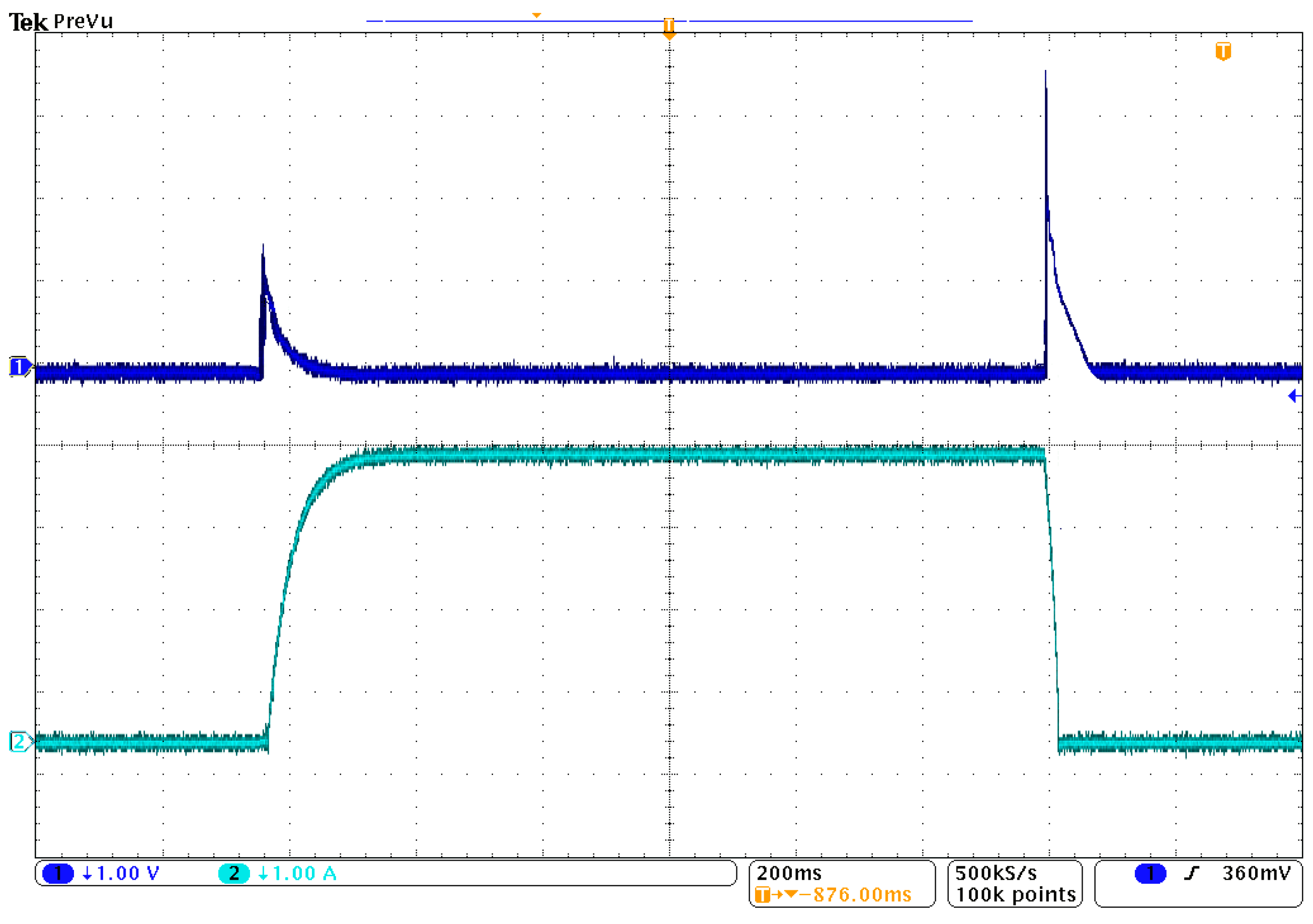
The digital simulations were verified experimentally by means of an ignition coil used to generate high voltages in typical ignition systems of spark-ignition engines. The tested coil was a circuit of two induction coils with an open ferromagnetic core of matching magnetization, as shown in Figure 8. The experimental tests consisted in recording the u₂(t) voltage at the system output for the input voltage in the form of a rectangular pulse. The recorded curves of u₂(t) voltage and i₁(t) current are shown in Figure 15.

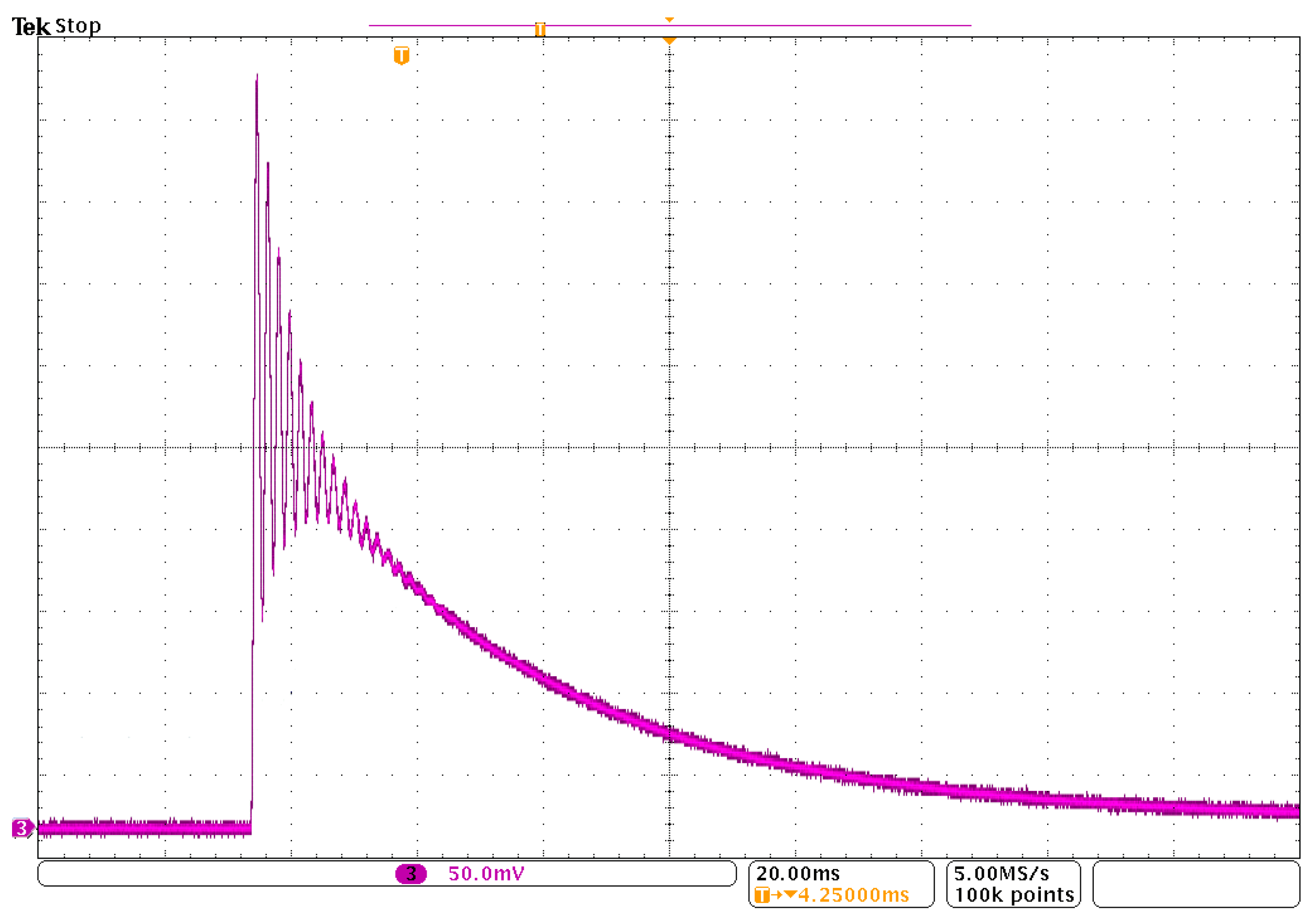
As can be seen, the curves of i₁(t) current and u₂(t) voltage obtained as a result of the experiments contain oscillations and are insignificantly different from the results of the numerical experiments shown in Figure 13 and Figure 14. In order to compare the experimental results with the simulations, a detailed curve of u₂(t) voltage at the moment of its induction for the fading impulse is presented in Figure 16.

The comparison of the obtained curve with the results of numerical simulations shows that the curves are similar in shape. The differences between the real and simulated curves result from the existence of micro-capacities in the tested circuit (e.g., between coils) and the capacity of the voltage probe used. Complementing the model of the circuit in Figure 8 with capacitive and resistive elements and then selecting α to make the model as close as possible to the real curves will allow for an accurate mathematical description of the analyzed circuit.

6. Conclusions

To sum up, it can be stated that the use of fractional-order magnetic coupling between two coils makes it possible to avoid the Dirac impulse that is used in the classical approach. In the case of first-order magnetic coupling (classical approach), the immediate appearance and immediate disappearance of voltage are assumed (Figure 3). In practice, no mechanical or even electronic switch is able to realize this state. The use of fractional-order magnetic coupling makes it possible to consider the non-ideality of coils and switches. Thus, results closer to those obtained experimentally can be achieved. In future studies, fractional-order magnetic coupling will be used to model the spark-ignition system of an internal combustion engine, and the results will be experimentally verified in a system with a standard ignition coil. As can be seen, the real curves presented in Figure 15 contain oscillations and are insignificantly different from the results of numerical experiments. The differences between the real and simulated curves result from the existence of micro-capacities (e.g., between coils) in the tested circuit. The next stage of research will include the development of a model containing capacitive and resistive elements and the selection of α to make the developed model as close as possible to the real curves.

An additional statement resulting from the study may be formulated as follows: The current waveform at the input of the electrical circuit is the same as with classical coupling, and the coupling value α considerably affects the value of voltage induced in the second coil. This means that the higher the α value, the “stronger” the coupling.