A Novel Risk-Based Prioritization Approach for Wireless Sensor Network Deployment in Pipeline Networks

Abstract

In the face of increased spatial distribution and a limited budget, monitoring critical regions of pipeline network is looked upon as an important part of condition monitoring through wireless sensor networks. To achieve this aim, it is necessary to target critical deployed regions rather than the available deployed ones. Unfortunately, the existing approaches face grave challenges due to the vulnerability of identification to human biases and errors. Here, we have proposed a novel approach to determine the criticality of different deployed regions by ranking them based on risk. The probability of occurrence of the failure event in each deployed region is estimated by spatial statistics to measure the uncertainty of risk. The severity of risk consequence is measured for each deployed region based on the total cost caused by failure events. At the same time, hypothesis testing is used before the application of the proposed approach. By validating the availability of the proposed approach, it provides a strong credible basis and the falsifiability for the analytical conclusion. Finally, a case study is used to validate the feasibility of our approach to identify the critical regions. The results of the case study have implications for understanding the spatial heterogeneity of the occurrence of failure in a pipeline network. Meanwhile, the spatial distribution of risk uncertainty is a useful priori knowledge on how to guide the random deployment of wireless sensors, rather than adopting the simple assumption that each sensor has an equal likelihood of being deployed at any location.

1. Introduction

With the application of condition based maintenance (CBM) in critical infrastructures, wireless sensor networks have gained so much popularity and are being deployed for sewage flood monitoring in sewer pipeline network, leakage monitoring in gas pipeline network, and strength monitoring of megastructures [1,2,3,4,5]. By delivering monitoring data, wireless sensor networks provide a key basis to help in assessing the assets’ or equipment’ condition, which is useful to guide the allocation of maintenance resource in time and space. In the dimension of time, the maintenance intervals are determined with the guidance. The interval initiates the maintenance actions such as the repair or replacement, which essentially allocates the resources in time dimension. For space, the guidance tells that where the parts of the critical infrastructure are likely to need maintenance. Based on that, initial limited maintenance resource can be target to the critical parts or regions. However, wireless sensor network deployment is a great challenge in pipeline networks. Despite the declining price of sensors, the cost remains high for the application, which requires hundreds and thousands of sensor nodes [6,7,8,9]. In the face of a limited budget and increased spatial distribution, a large-scale deployment of a wireless sensor network is impossible to implement for a whole pipeline network [10]. Budget constraints only allow a limited part of a pipeline network to be deployed. Therefore, the key problem is to identify the regions where the necessity of their deployments of wireless sensor network is more important than the availability.

To the best of our knowledge, there is no effective approach to address the issue. First of all, the key problem is different from the coverage problems which is the most similar one among the current research problems. In general, coverage problems are classified into three categories—point coverage problem, area coverage problem, and barrier coverage problem. No matter which type the problem is, the problem is essentially an optimization. The objective is to determine which deployment strategy for a specified sensor field can achieve the maximum utility of a wireless sensor network with constraints such as the number of sensor nodes, the area covered by the wireless sensor network, or the lifetime of sensors [11,12,13,14,15]. However, our problem needs to determine which parts of the specified sensor field are prioritized for deployment. Essentially, this is a sort rather than an optimization. Next in importance was that our problem originates from the invalidation of the common assumption used by many existing approaches. No matter which deployment method is applied, deterministic deployment or random deployment, there is a predetermined sensor field underpinning it. Based on the assumption on the predetermined sensor field, we can calculate coverage ratio, which is often regarded as one of the coverage requirements for wireless sensor networks [16]. However, there is no a predetermined sensor field in our problem. We have no idea about the location, boundary, or area of the sensor field, and all the attributes need us to determine when we know which parts of the specified sensor field are prioritized for deployment. Finally, the current primary deployment metrics are not suitable. In a pipeline network, wireless sensor network deployment is an application in industrial diagnostics; its coverage requirements can fall into the target coverage category [17,18,19,20]. Those requirements are used to measure the quality of service of the sensors’ sensing function provided by determining how to deploy the sensor network. In our problem, we were concerned with how to measure the value realized by determining whether or not to deploy a sensor network. In conclusion, we need to develop a methodology for addressing the issue.

In this study, we tried to develop an approach to address this challenge. Our approach was based on risk-based prioritization. Through risk-based prioritization, stakeholders are able to target resources where parts of a pipeline network have a high risk. Therefore, resources can be utilized in a more effective and efficient manner [21]. Risk-based prioritization originates from a risk-based inspection project, which was started by the American Petroleum Institute (API) [22,23,24]. Subsequently, the idea has been applied widely in different industrial contexts, such as in the nuclear industry in order to prioritize maintenance [25,26,27,28], gas pipelines to guide the allocation of maintenance resources on the most risky stretches of pipeline [29], the optimization of the maintenance of water supply networks [30], and the risk ranking procedure for bridges [31]. However, limitations can be observed when they are applied in the wireless sensor network deployment of pipeline networks.

First of all, it is not beneficial for a pipeline network to execute the second step of the whole deployment plan of a wireless sensor network in practice. As mentioned above, the wireless sensor network deployment can be seen as a two-step process in pipeline networks:

• Sorting—identifying the critical regions by ranking different deployment regions in terms of risk;
• Optimizing—determining the deployment strategy in order to achieve the maximum utility of a wireless sensor network.

In the second step, for each optimization the geographical environment of the installation, the signal interference around the sensor nodes, the area of coverage, and other spatial constraints should be kept in mind. In the deployment of pipeline networks, the optimization needs to be conducted in a given area or length, because the coverage ratio needs to be calculated to measure the quality of service of the wireless sensor network. Risk-based prioritization is required to consider the factors quantitatively. However, the current approach of risk-based prioritization cannot achieve the aim [32].

Furthermore, many stakeholders are often not satisfied with the result, because the analysis process does not provide a strong credible basis for the estimation of risk uncertainty. In a pipeline network, a wireless sensor network is used to detect failure events at some location. Risk uncertainty can describe where the failure event is more likely to occur. According to the estimation of risk uncertainty, we can deploy the sensor nodes efficiently in order to avoid the situation so that considerably more regions are available than necessary for monitoring. Unfortunately, the used assumptions and hypotheses in many approaches cannot be proven right or wrong in the estimation [33]. This leaves the assessment of risk uncertainty to be based on the degree of belief of the assessors. Therefore, decision makers do not gain any confidence from the analysis, which, in particular, relies on the assessment of uncertainty based on the subjective judgments of the assessors.

Against these backdrops, some improvements can be achieved based on risk-based prioritization in our proposed approach. The advantages of the proposed approach are as follows:

• Our approach combines risk-based prioritization with spatial statistics, which quantitatively estimates risk of any geographic region where the pipeline network located with the consideration of the area of the region. It is very useful for the second step to be executed when the deployment/placement scheme is required to be assessed based on coverage ratio;
• Statistical tests are applied before modelling, which provide a strong credible basis for the estimation of risk uncertainty. It is valuable for engineers to determine the deployed region with consideration of the effect of condition monitoring, in particular, detecting the failure events.

The total cost caused by failures in each deployment region is calculated to measure the severity of risk. Then the risks of different deployment regions are calculated based on the severity and uncertainty. By sorting the risks, high risk regions are identified. This allows the deployment of the wireless sensor network to be guided.

The rest of this paper is structured as follows: Section 2 presents our method, including all the relevant statistical tests and steps for risk-based prioritization; Section 3 shares a real case study, which examines the availability of our method, and the process and outcomes are detailed; and finally, Section 4 concludes the paper and outlines future work.

2. Method

To suggest better practice for wireless sensor network deployment, our approach is represented in a rigorous and confident manner, as shown in Figure 1. Three statistic tests were first conducted in two stages, which guaranteed that the inhomogeneous Poisson point process is a rational application for modelling the location dataset of pipeline failure events. Based on that, the properties of the inhomogeneous Poisson point process were applied to estimate the probability of the failure occurrence in different deployment regions. Afterwards, the rest of the procedures of risk-based prioritization were executed, and the risks in different deployment regions were obtained. Finally, the different deployment regions were ranked in the order of risk.

2.1. Inhomogeneous Poisson Point Process

There is a growing body of contemporary data about where an individual pipeline failure event occurs. It provides new opportunities to study the spatial pattern of failure occurrence in a pipeline network. The observed spatial locations of the failure events in a pipeline network can be viewed as data in the form of a set of points, irregularly distributed within a region of space (as is shown in Figure 2). As one of the spatial statistics technologies, spatial point process is widely used to analyze spatial point data [34,35,36]. The inhomogeneous Poisson point process, being one of the models in the spatial point process [37,38,39], was applied in our approach to assess the uncertainty of risk.

An inhomogeneous Poisson point process, $N$, is a random mechanism whose outcomes are a point pattern, $X$. In our approach, the element, $x$, of the point pattern, $X$, represents the location of the failure event. The location of the failure event is generally referenced using a geographical coordinate. For any region, $B$, such as the region of Kansas in Figure 2, the number of failure events occurring in it, $n(X\cap B)$, is a well-defined random variable. Based on the quantity, the inhomogeneous Poisson point process is often characterized by two fundamental properties:

• Poisson Counts—the number of failure events, $n(X\cap B)$, has a Poisson distribution;
• Independent—if parts of Region $B$ are $B_1$, $B_2$,…, $B_m$, which do not overlap, the counts $n(X\cap B_1)$,…, $n(X\cap B_m)$ are independent random variables.

According to the properties, the probability of observing $k$ failure events occurring in any region, $B_i$, can be described by the Poisson distribution, which is generally represented as Equation (1). The quantity $\Lambda$ is the expected number of failure events occurring in Region $B_i$, which is calculated by Equation (2) with the intensity $\lambda (x)$. The intensity is interpreted as the average number of failure events occurring per unit area. If the intensity is spatially varying, it is called an inhomogeneous Poisson point process, which is used to distinguish from the homogeneous Poisson point process where the intensity is constant. The difference between the homogeneous and inhomogeneous Poisson point processes can be observed in Figure 3.

$$p\{n(X\cap B_i)=k\}=e^{-\Lambda }\frac{{\Lambda }^k}{k!}$$

(1)

$$\Lambda ={\displaystyle \underset{B_i}{\int }\lambda (x)dx}$$

(2)

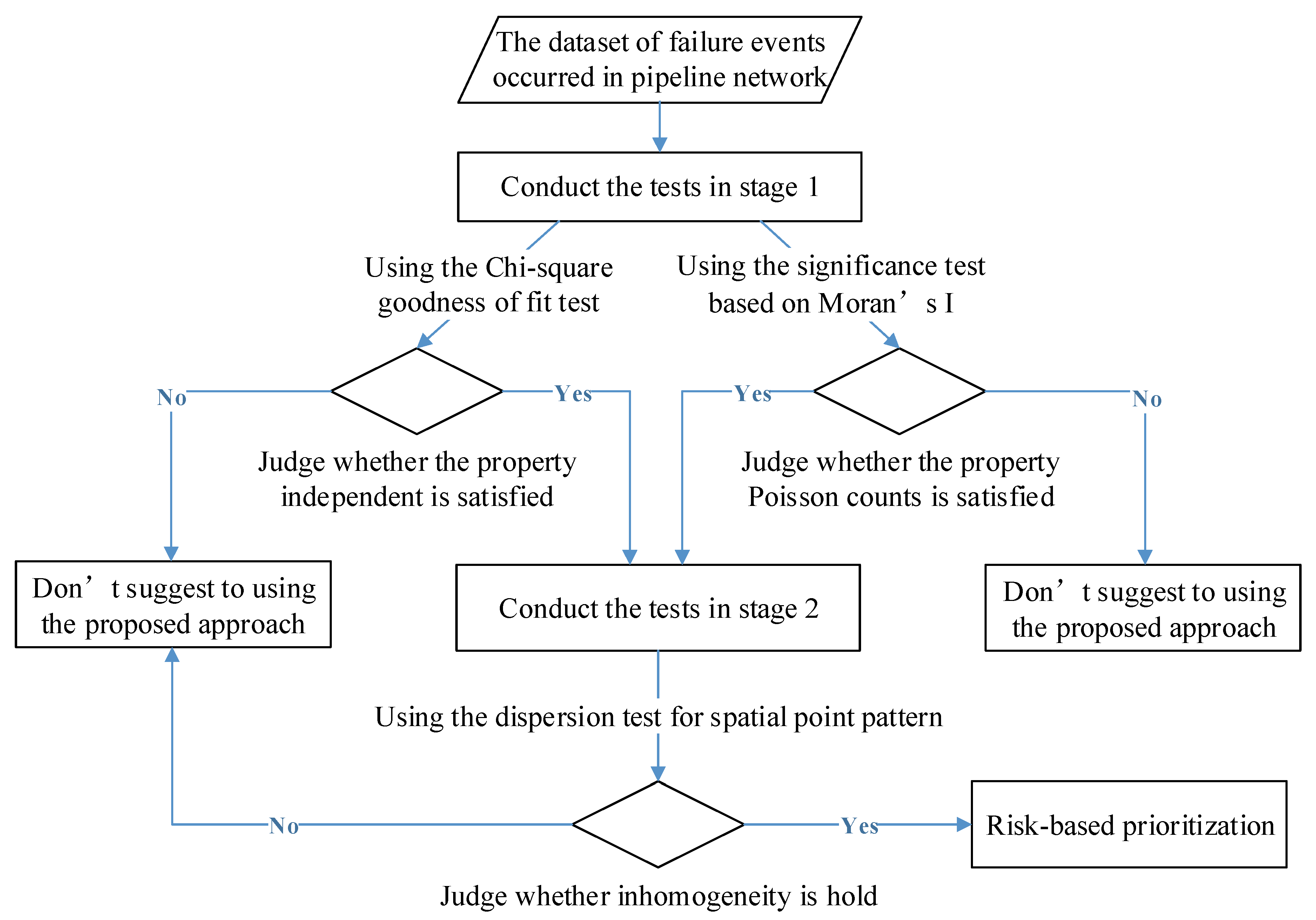
2.2. Statistical Tests for Inhomogeneous Poisson Point Process

In order to describe a real dataset of pipeline network failures well, through the inhomogeneous Poisson point process, our approach was to verify the relevant properties of the inhomogeneous Poisson point process using three hypothesis tests in two stages. In stage one, the Poisson counts and independent properties were respectively verified by the chi-square goodness of fit test [40,41,42] and the significance test based on Moran’s I [43,44,45]. This concluded that the Poisson point process was a suitable model for the dataset in stage one. The conclusion should be subject to further review on whether the intensity of the failure event was spatially varying (i.e., whether the Poisson point process is homogeneous or inhomogeneous). Therefore, a dispersion test for spatial point pattern was conducted in stage two [46] to determine whether the suitable model for pipeline failure events was the inhomogeneous Poisson point process rather than the homogeneous Poisson point process.

2.2.1. First Test in Stage One: Chi-Square Goodness of Fit Test

To determine whether the property Poisson counts were held, a chi-square goodness of fit test was required to determine whether the data followed a specific probability distribution. In this hypothesis test, the null and alternative hypotheses were as follows:

• H₀: the number of pipeline failure events in Region $B$ and a given period, $t$, follows a Poisson distribution;
• H₁: the number of pipeline failure events in Region $B$ and a given period, $t$, does not follow a Poisson distribution.

Using Equation (3), the mean $\Lambda$ of Poisson distribution was estimated based on the sample data like those shown in

Table 1. Frequency distribution of the number of pipeline failure events per month in Kansas.

Number of Failure Events Per Month ($\mathit{k}$)	Observed Frequency (${\mathit{f}}_{\mathit{i}})$
0	18
1	28
2	17
3	11
4	6
5	3
6	0
7	1

. The sample data described the actual failure number per the given period. Based on that, a Poisson distribution with the estimated mean $\Lambda$ was obtained, and the theoretical frequency, $f_e$, was calculated by multiplying the sample size, $n$, and its probability, $p\{n=k\}$. Then the ${\chi }^2$ test statistic was obtained by Equation (4). By comparing the ${\chi }^2$ test statistic, we could determine whether to reject H_0. If the null hypothesis is rejected, the proposed approach is not suggested to be used because the Poisson point process is not a suitable model for the dataset. If the null hypothesis is accepted, it should continue to implement the next steps.

$$\Lambda =\frac{{\displaystyle \sum _{j=1}^c{m}_j{f}_i}}{n}$$

(3)

where $c$ is the number of classes of the number of failure events, $m_j$ is the number of failure events of the jth class, $f_i$ is the observed frequency, and $n$ is the sample size

$${\chi }_{\kappa -p-1}={\displaystyle \sum _{\kappa }\frac{{(f_i-f_e)}^2}{f_e}}$$

(4)

where $f$ is the theoretical frequency, $\kappa$ generally equals $c+1$ and $p$ is the number of parameters estimated from the sample.

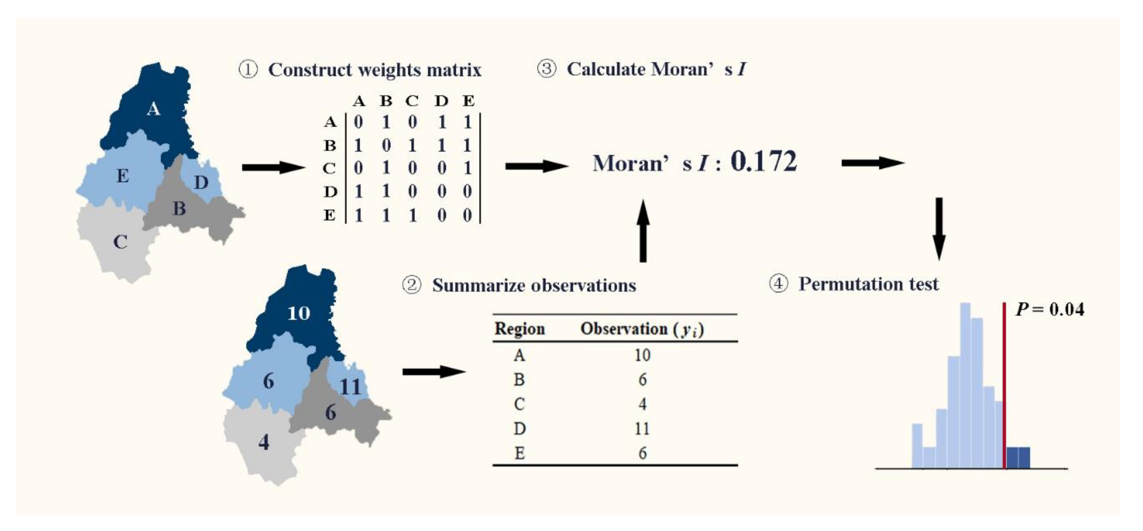
2.2.2. Second Test in Stage One: The Significance Test Based on Moran’s I

The second test in stage one inspected whether or not the numbers of failure events in different parts of Region $B$ appear to be correlated. The first step in this procedure was to calculate the observed value of Moran’s I based on the pipeline network failure dataset, then a significance test was performed to determine whether the observed value of Moran’s I differed enough from the value that was expected from where the independent property was held. Figure 4 illustrates the process based on a simple example.

As a commonly used spatial statistic to describe spatial autocorrelation, Moran’s I measures the degree to which observations (the number of pipeline failure events in this study) at different spatial locations (the different regions or parts of a pipeline network in this study) are similar to each other. Its calculation is based on two categories of information—the observation and the location. Here, the observation information included the numbers of pipeline failure events in different regions, often denoted by $y_i$ for Region i. The location information is represented by a spatial weights matrix, and the dimensions of it are $N\times N$ ($N$ being the number of regions). Here, the element of the spatial weights matrix, $w_{i,j}$, reflected the level of spatial proximity in two different regions of pipeline network, which is generally given by 1 if Regions i and j are neighbors and 0 otherwise. With both observation and location information, the observed value of Moran’s I can be calculated by Equation (5). In general, the observed value of Moran’s I will be compared with the expected value of Moran’s I. The expected value of Moran’s I can be obtained by $-\frac{1}{N-1}$. If the observed value of Moran’s I were significantly larger than the expected value of Moran’s I, it indicates a positive spatial autocorrelation; If the observed value of Moran’s I were significantly less than the expected value of Moran’s I, it indicates a negative spatial autocorrelation. If there were no significant difference between the observed value of Moran’s I and the expected value of Moran’s I, it indicates a spatial independence.

$$I=\frac{N}{{\displaystyle \sum _{i=1}^N{(y_i-\overline{y})}^2}}\frac{{\displaystyle \sum _{i=1}^N{\displaystyle \sum _{j=1}^{N,i\ne j}{w}_{i,j}(y_i-\overline{y})(yi-\overline{y})}}}{{\displaystyle \sum _{i=1}^N{\displaystyle \sum _{j=1}^{N,i\ne j}{w}_{i,j}}}}$$

(5)

where $\overline{y}$ is the mean of $y$.

In the second step, a significance test is performed. The null and alternative hypotheses were defined as follows:

• H₀: the number of pipeline failure events in different regions are spatially independent;
• H₁: the number of pipeline failure events in different regions are spatially dependent.

The null hypothesis stated that the numbers of failure events in different regions of pipeline network will be randomly distributed among those regions. Under the null hypothesis, the distribution of the test statistic Moran’s I was obtained by calculating all possible values of Moran’s I under rearrangements of the numbers of pipeline failure events on all the regions. Imagine that all the failure numbers in different regions are picked up and thrown down onto all the regions again, with each number falling randomly. The proportion is obtained by counting how many permuted Moran’s I are larger than the observed value of Moran’s I, which is a p-value. Finally, a decision must be made to accept the null or alternative hypothesis according to the level of significance. If the null hypothesis is rejected, the proposed approach is not suggested to be used because the Poisson point process is not a suitable model for the dataset. If the null hypothesis is accepted, it should continue to implement the next steps.

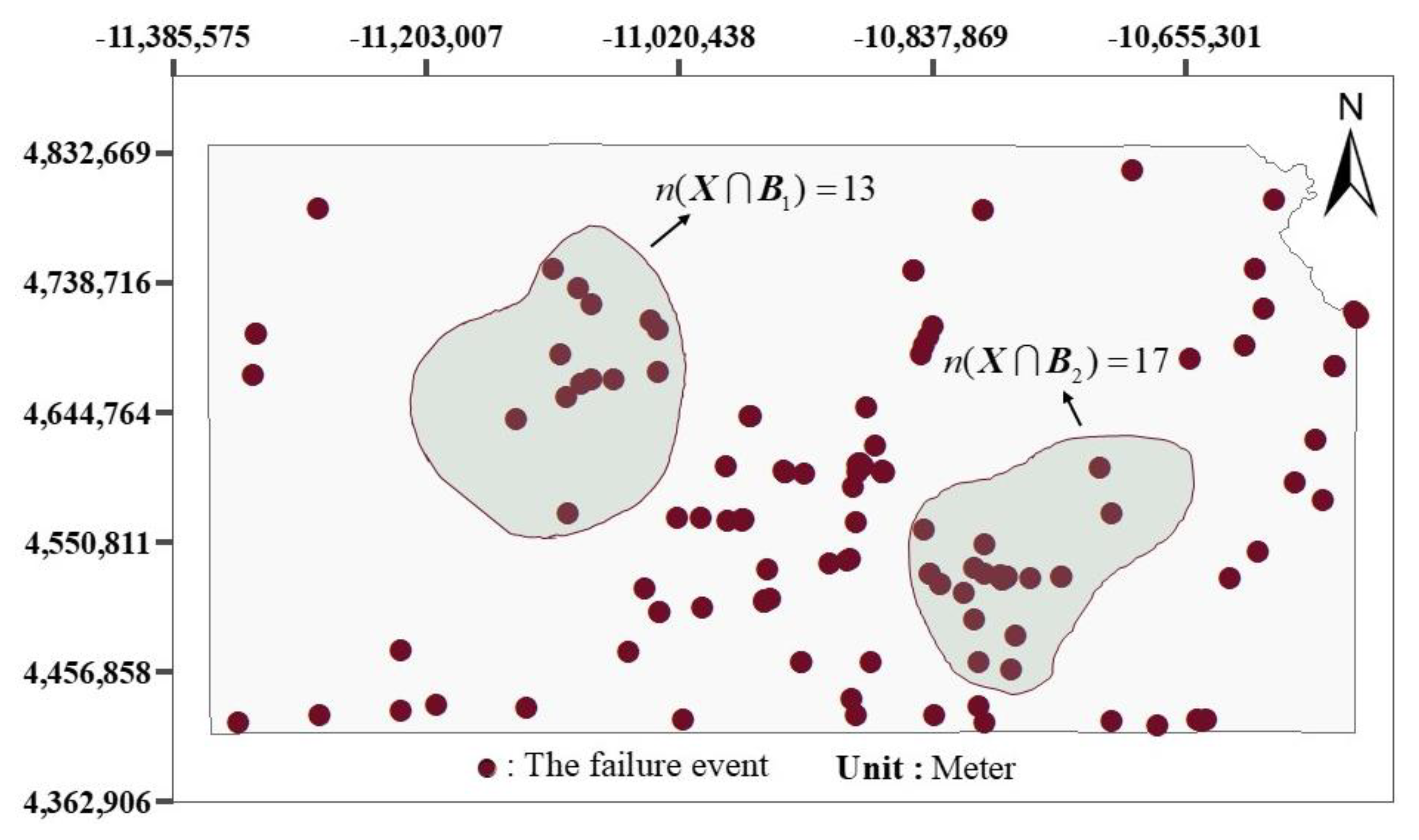
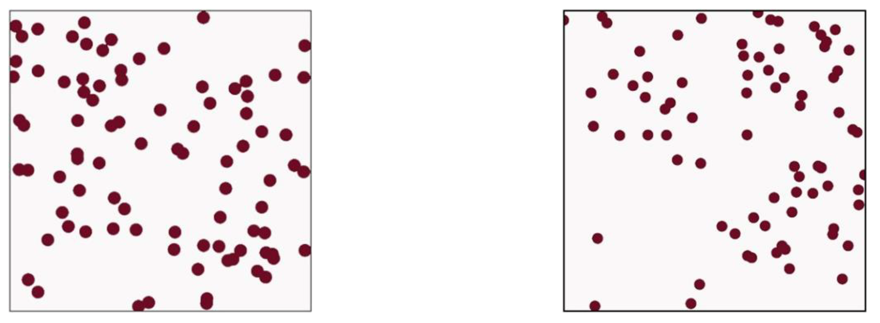
2.2.3. Test in Stage Two: The Dispersion Test for Spatial Point Pattern Based on Quadrat Counts

Although it can be concluded that the Poisson point process is a suitable model for the dataset of pipeline failure events after stage one, the evidence for inhomogeneity needed to be assessed. Therefore, a dispersion test for spatial point pattern based on quadrat counts was conducted in stage two, which essentially is a chi-squared test to test goodness of fit. It guaranteed that the inhomogeneous Poisson point process is a suitable model, rather than homogeneous Poisson point process.

In the dispersion test for spatial point pattern based on quadrat counts, the quadrats represented the regions nominated to be deployed in a pipeline network, and they were required to have an equal area, $a$. Generally, the null and alternative hypotheses in the test were defined as:

• H₀: the intensity is homogeneous in the Poisson point process based on the dataset of pipeline failure events;
• H₁: the intensity is inhomogeneous in the Poisson point process based on the dataset of pipeline failure events.

According to the null hypothesis and Equation (2), the numbers of failure events in different quadrats were realizations of Poisson distribution with the constant mean, $\lambda a$. Therefore, it was rational to apply the chi-squared test to test goodness of fit to the Poisson distribution to determine whether or not to reject the null hypothesis.

The test statistic can be calculated by Equation (6). In Equation (6), the quantity, $n_j$, is the number of failure events in Region $B_j$ (or the quadrat), and the distribution of the test statistic is approximately a ${\chi }^2$ distribution with $m-1$ degrees of freedom ($m$ is the total number of regions nominated to be deployed). By performing a chi-squared test, it could be determined whether or not to reject the null hypothesis.

$$X={\displaystyle \sum _j\frac{{(n_j-\overline{\lambda }{a}_j)}^2}{\overline{\lambda }{a}_j}}$$

(6)

where the intensity $\overline{\lambda }$ is estimated by $\overline{\lambda }=\frac{n}{a}$ and the total number of points is $n={\displaystyle \sum _j{n}_j}$.

2.3. Risk-Based Prioritization

By the verification above, there is no reason to doubt that the inhomogeneous Poisson point process is a good model for the failure events of a pipeline network. Based on that, the probability of the failure occurrence in different regions can be estimated. According to Equation (1), the probability of the failure event occurring in Region $B_j$ can be represented as Equation (8). To calculate the mean value of this Poisson distribution $\Lambda$, the integral in Equation (2) is replaced by $\Lambda =\overline{{\lambda }_{B_j}}\left|B_j\right|$, which assumes that the intensity in Region $B_j$ is homogeneous, but the intensity of the whole pipeline network is inhomogeneous. Based on this assumption, the intensity $\overline{{\lambda }_{B_j}}$ can be estimated by Equation (7). Although the number of failure events in a pipeline network follows a Poisson distribution, it is worth noting that it was observed under a specified period. Therefore, the probability ${\mathrm{P}(\mathrm{U}}_{B_j})$ should be revised as ${\mathrm{P}(\mathrm{U}}_{B_j}|\mathrm{T}<t)$.

$$\overline{{\lambda }_{B_j}}=\frac{n(X\cap B_j)}{\left|B_j\right|}$$

(7)

$${\mathrm{P}(\mathrm{U}}_{B_j})=\mathrm{P}\{N\ge 1\}=1-\mathrm{P}\{N=0\}=1-e^{-\Lambda }\frac{{\Lambda }^N}{N!}=1-e^{-\Lambda }$$

(8)

After the estimation of the probability of the failure occurrence in different regions, the consequence of the failure occurrence is evaluated in different regions. In our approach, the consequence of the failure occurrence is measured by the total cost for the region $B_j$, which is denoted by $C_{B_j}$. The total cost $C_{B_j}$ is calculated based on the summarization of the cost of the failure event happens in each region. The cost of each failure event is constituted by six kinds of costs, which is described in

Table 2. Constitution of the cost of each failure event.

No.	Cost
1	Property Damage Costs
2	Lost Commodity Costs
3	Public/Private Property Damage Costs
4	Emergency Response Costs
5	Environmental Remediation Costs
6	Other Costs

. Based on the six kinds of costs, the assessment of the failure consequence can consider the capacity of the failure and subsequent events to cause death, injury, or damage to employees and/or the public and the environment. Apart from that, it can also consider the consequences of failure on the business, such as the costs of lost production, repair and replacement of pipeline, and the damage to the company reputation.

With the estimated probability and the evaluated consequence, the risk can be determined. In the proposed approach, the risk of each region is defined as the product of the probability and the consequences of the failure occurrence. Based on the obtained risk, all the regions can be ranked in order of risk, then the deployment priority can be given to each region.

3. Case Study

In this section, we describe a case study of the wireless sensor network deployment in the Kansas state pipeline network. The area of the whole pipeline network is 346,647.9 km², which has approximately 47,388 miles of pipeline. In this case study, sixteen sensor fields are required to get the right priority of wireless sensor network deployment by using the proposed approach. The data used in the case study were provided by the Pipeline and Hazardous Materials Safety Administration (PHMSA). They included 141 failure events of pipeline across Kansas during 2010–2016, and the spatial distribution of those failure events is shown in Figure 2. The information about each failure event contained in the data is described in

Table 3. Information about each failure event contained in the data.

Attribution	Description
Failure location	The location of the failure occurrence of pipeline network, which is represented in terms of latitude and longitude.
Failure time	The time of the failure occurrence in the pipeline network
Failure cause	The cause of failure
Total cost	The total cost caused by the consequence of each pipeline failure

. The identification number and the number of failure events that occurred in each sensor field are illustrated in Figure 5.

3.1. Statistical Tests for Inhomogeneous Poisson Point Process

As mentioned above, the first test in stage one is the chi-square goodness of fit test. It determines whether the number of pipeline failure events follow a Poisson distribution. Before the hypothesis test, the actual number of failure events was counted under a given period, which is shown in Table 1. The given period was one month. The level of significance was set to be 0.05. Using the Equation (4), the critical value of ${\chi }^2$ is obtained, which was 10.006. Based on that, the decision rule was defined as:

$$\mathrm{Reject}{H}_0\mathrm{if}{\chi }^2>14.067,\mathrm{otherwise}\mathrm{do}\mathrm{not}\mathrm{reject}{H}_0.$$

Through performing the test, the decision was not to reject H₀ since ${\chi }^2=10.006<14.067$. There was insufficient evidence to conclude that the number of failure events that occurred monthly in Kansas did not fit the Poisson distribution.

The second test in stage one is the significance test based on Moran’s I, where the independent property is inspected. The number of failure events that occurred in each region can be checked in Figure 5, and the spatial weights matrix is shown in Figure 6. Based on that, the computation of Moran’s I and a significance test were implemented. The result is summarized in

Table 4. Results of the significance test based on Moran’s I.

Statistic	Result
Moran’s Index	0.055905
Expected Moran’s Index	−0.066667
Z-score	1.153184
P-value	0.248577

. Although the observed value of Moran’s I was larger than the expected value, the p-value was not statistically significant. It means that there is no significant difference between the observed value of Moran’s I and the expected value of Moran’s I. Therefore, the null hypothesis could not be rejected. It is quite possible that the number of failure events in different regions was the result of randomness. Therefore, we think the independent property was held.

In stage two, the evidence for inhomogeneity was assessed by a dispersion test for spatial point pattern. The numbers of failure events falling into those regions can be checked in Figure 5. The area of each region is listed in

Table 5. Area of each region.

Region ID	Area (km2)	Region ID	Area (km2)	Region ID	Area (km2)	Region ID	Area (km2)
1	21810.48	5	22064.53	9	22095.08	13	22034.45
2	21906.91	6	22136.67	10	22136.67	14	22046.50
3	21847.71	7	22136.67	11	22136.67	15	21962.08
4	21612.80	8	21936.47	12	21720.03	16	17064.15

, and we think it is rational to assume that all the regions have an approximately equal area. Due to the null hypothesis, i.e., the intensity is homogeneous, the estimation of it was 4.07E-04 times per square kilometer by the equation ${\displaystyle \sum _i{n}_i}/{\displaystyle \sum _i{a}_i}$. Through the implementation of the test, we saw that the test rejected the null hypothesis by inspecting the p-value of 2.2E-16. Therefore, it was reasonable for the dataset to be analyzed under the assumption of inhomogeneity.

3.2. Risk-Based Prioritization

Based on the verification above, the probability of the failure event occurring was estimated for each region according to the equations in Section 2.3. To calculate the total cost of each region, the total cost of each failure event in a region was added together to give the total cost of the region according to the items of total cost listed in Table 3. With all the information above, the risk in each region was evaluated by the production of the probability of failure, ${\mathrm{P}(\mathrm{U}}_{B_j}|\mathrm{T}<t)$, and the measure of the consequence, $C_{B_j}$. According to the results, each region was ranked based on its risk.

3.3. Results and Discussion

After the implementation of all the steps above, the total cost and the probability of failure occurrence were estimated respectively for all sensor fields, and the risks of them were calculated. All the sensor fields were ranked based on their risks. All the results can be observed in

Table 6. The results.

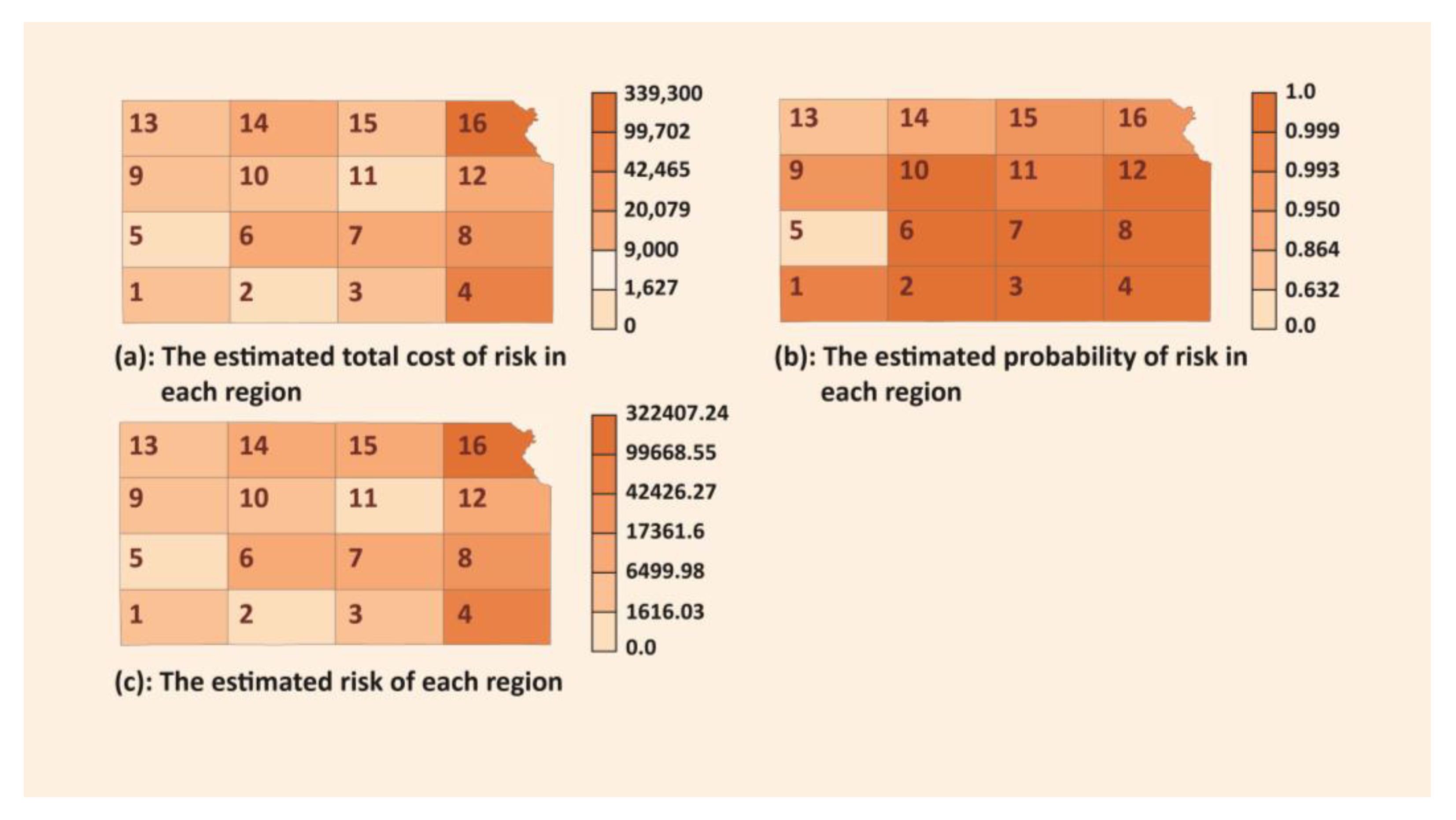
Region ID	Cost ($)	Rank	Probability	Rank	Risk	Rank
16	339300	1	0.950213	12	322407	1
4	99702	2	0.999665	7	99668.6	2
8	42465	3	0.999088	8	42426.3	3
14	20079	4	0.864665	14	17361.6	4
12	13110	5	0.999983	5	13109.8	5
7	12150	6	1	1	12150	6
6	11012	7	0.999877	6	11010.6	7
15	9000	8	0.950213	11	8551.92	8
3	6500	9	0.999998	2	6499.99	9
9	4750	10	0.950213	13	4513.51	10
10	3880	12	0.999994	3	3879.98	11
1	3510	13	0.993262	10	3486.35	12
13	3888	11	0.632121	15	2457.68	13
11	1627	14	0.993262	9	1616.04	14
2	300	15	0.999994	4	299.998	15
5	0	16	0	16	0	16

. To provide a better conveyance of information in results, the result of each sensor field are arranged in Table 6 according to the index which is calculated by Equation (9). In Equation (9), the cost, probability and risk are respectively the total cost, the estimated probability of failure occurrence and the risk of every sensor field. According to the ranks in Table 6, every sensor field was given its priority of wireless sensor network deployment. The critical regions were identified based on the priority. Stakeholders would be able to target the initial deployment where the application of a wireless sensor network is necessary. Therefore, the limited efforts and resources of wireless sensor networks can be utilized in a more effective and economic manner by our approach.

$$\mathrm{Index}=\mathrm{Cos}\mathrm{t}\times 25\%+\mathrm{Probability}\times 25\%+\mathrm{Risk}\times 50\%$$

(9)

On top of that, the result was obtained with the consideration of the area of the sensor field. Based on the critical sensor density (the minimal required number of nodes per unit area for complete area coverage), the information on the area was very helpful in deciding how many nodes would be needed to completely cover the sensor field. Then, the deployment cost of every sensor field could be reasonably estimated. At the same time, we can view the calculated risk as the expected loss occurring in each sensor field [47]. We can determine the economy of the wireless sensor deployment in each sensor field through a comparison with the deployment cost. Therefore, by observing the spatial distribution of risk in Figure 7c, wireless sensor network deployment in some regions would be more economic than in others, such as Sensor Fields 16 and 4.

If stakeholders focus on the requirement of target coverage, sensors should be dispatched to the sensor field where failure events occur frequently, such as in Regions 1, 2, 3, 4, 6, 7, 8, 10, and 12. As is shown in Figure 7b, the estimated probabilities in all the sensor fields provide a distribution. The distribution describes where the failure events are likely to take place. This is very useful information on event sources in target coverage. If the requirements are related to target coverage, deploying wireless sensors in those regions enables the collection of more data on the pipeline failure. These data would be very useful to improve detection algorithms.

Furthermore, we found that the spatial distribution of the likelihood of failure occurrence has spatial heterogeneity. The spatial variation of risk uncertainty is obvious by observing Figure 7b. This discovery provides guidance for random deployment in the whole state, if the stakeholders had an adequate budget. The spatial distribution of the likelihood of failure can be adopted as a reference distribution for deployment when the random deployment is applied for wireless sensor network in the whole state. This provides a priori knowledge on how to scatter sensors randomly, rather than the simple assumption that each sensor field has an equal likelihood of scattering in everywhere. This is helpful to avoid an inadequate wireless sensor network deployment in random deployment.

4. Conclusions

The result in the case study shows that the proposed approach is feasible for a pipeline network to reasonably direct a wireless sensor network to deploy critical sensor fields in the face of a limited budget and increased spatial distribution. By combining spatial statistics with risk-based prioritization, our approach is effective in identifying the sensor fields with the highest priority in a pipeline network, which is useful to target the initial deployment where the sensor field is necessary rather than available. Additionally, the application of statistical tests provides a strong credible basis for the analytical conclusion, which is very different from the existing methods whose conclusions are based on the subjective judgments of assessors. Moreover, the analytical conclusion is very helpful for the coverage problem and for developing the deployment strategy further. More importantly, we gained insight from the case study, which the spatial distribution of the likelihood of failure occurrence in a pipeline network has spatial heterogeneity. The spatial and geographical variations are useful a priori knowledge on how to guide the deployment of wireless sensors, rather than adopting the simple assumption that each sensor field has an equal likelihood of being deployed.

At the same time, the limitations can be observed in the proposed approach. First of all, the proposed approach cannot consider the characteristics of pipelines such as the diameters, the flow, and the failure modes. The reason why brings about the limitations is the transformation of the modeled object from a stretch or a section of pipeline to the whole district where pipeline network located. In the process of transformation, the spatial coordinates become the surrogate for other variables that report failure modes and system characteristics. Thus, many characteristics in components level or system level cannot be modeled although it overcomes the difficulty of insufficient data by the aggregation of the rarely failure events which belongs to the different sections of pipeline that dispersed in different positions of the industry infrastructure. Next in importance is the strict constrains of the application, which is the validations of properties of Poisson point process, which is a double-edged sword. Although the validations increase the falsifiability of the proposed approach and reduce the vulnerability to human biases and errors, the availability of our approach is significantly decreased by the validations if those properties are violated. Therefore, users should apply the proposed approach in the appropriate situation.

In the future, we plan to incorporate some other statistical technologies to estimate the risks of different sensor fields that are conditional on different failure modes. Based on that, the approach will not only be useful for homogeneous deployment but will also guide the heterogeneous deployment of wireless sensor networks.

References

- Cheklat, L.; Amad, M.; Boukerram, A. Wireless Sensor Networks, State of Art and Recent Challenges: A Survey. Sens. Lett. 2017, 15, 697–719. [Google Scholar] [CrossRef]
- Modieginyane, K.M.; Letswamotse, B.B.; Malekian, R.; Abu-Mahfouz, A.M. Software defined wireless sensor networks application opportunities for efficient network management: A survey. Comput. Electr. Eng. 2018, 66, 274–287. [Google Scholar] [CrossRef]
- Martini, A.; Rivola, A.; Troncossi, M. Autocorrelation Analysis of Vibro-Acoustic Signals Measured in a Test Field for Water Leak Detection. Appl. Sci. 2018, 8, 2450. [Google Scholar] [CrossRef]
- Yazdekhasti, S.; Piratla, K.R.; Atamturktur, S.; Khan, A. Experimental evaluation of a vibration-based leak detection technique for water pipelines. Struct. Infrastruct. Eng. 2017, 14, 46–55. [Google Scholar] [CrossRef]
- Martini, A.; Troncossi, M.; Rivola, A. Vibroacoustic Measurements for Detecting Water Leaks in Buried Small-Diameter Plastic Pipes. J. Pipeline Syst. Eng. Pr. 2017, 8, 04017022. [Google Scholar] [CrossRef]
- Ali, A.; Mihaylova, L.; Adebisi, B.; Ikpehai, A. Location prediction optimisation in WSNs using Kriging interpolation. IET Wirel. Sens. Syst. 2016, 6, 74–81. [Google Scholar] [CrossRef]
- Aguiar, E.F.K.; Roig, H.L.; Mancini, L.H.; De Carvalho, E.N.C.B. Low-Cost Sensors Calibration for Monitoring Air Quality in the Federal District—Brazil. J. Environ. Prot. 2015, 6, 173–189. [Google Scholar] [CrossRef]
- Sivaraman, V.; Carrapetta, J.; Hu, K.; Luxan, B.G. HazeWatch: A participatory sensor system for monitoring air pollution in Sydney. In Proceedings of the 38th Annual IEEE Conference on Local Computer Networks—Workshops, Sydney, NSW, Australia, 21–24 October 2013; pp. 56–64. [Google Scholar]
- Carrapetta, J. Haze Watch: Design of a Wireless Sensor Board for Measuring Air Pollution. Ph.D. Thesis, School of Electrical Engineering and Telecommunications, Sydney, NSW, Australia, 2010. [Google Scholar]
- Marlow, D.; Beale, D.J.; Burn, S. A pathway to a more sustainable water sector: Sustainability-based asset management. Water Sci. Technol. 2010, 61, 1245–1255. [Google Scholar] [CrossRef]
- Aznoli, F.; Navimipour, N.J. Deployment Strategies in the Wireless Sensor Networks: Systematic Literature Review, Classification, and Current Trends. Wirel. Pers. Commun. 2016, 95, 819–846. [Google Scholar] [CrossRef]
- Rashid, B.; Rehmani, M.H. Applications of wireless sensor networks for urban areas: A survey. J. Netw. Comput. Appl. 2016, 60, 192–219. [Google Scholar] [CrossRef]
- Stoianov, I.; Nachman, L.; Madden, S.; Tokmouline, T. PIPENETa wireless sensor network for pipeline monitoring. In Proceedings of the 6th International Conference on Multimodal Interfaces—ICMI ’04, Porto, Portugal, 9–13 September 2007; p. 264. [Google Scholar]
- Wang, C.; Wang, B.; Liu, W. Movement strategies for improving barrier coverage in wireless sensor networks: A survey. In Proceedings of the 2011 IEEE 13th International Conference on Communication Technology, Jinan, China, 25–28 September 2011; pp. 938–943. [Google Scholar]
- Liu, Y.; Ma, X.; Li, Y.; Tie, Y.; Zhang, Y.; Gao, J. Water Pipeline Leakage Detection Based on Machine Learning and Wireless Sensor Networks. Sensors 2019, 19, 5086. [Google Scholar] [CrossRef] [PubMed]
- Wang, B. Coverage problems in sensor networks. ACM Comput. Surv. 2011, 43, 1–53. [Google Scholar] [CrossRef]
- Mini, S.; Udgata, S.; Sabat, S. Sensor Deployment and Scheduling for Target Coverage Problem in Wireless Sensor Networks. IEEE Sens. J. 2013, 14, 636–644. [Google Scholar] [CrossRef]
- Chaudhary, M.; Pujari, A.K. Q-Coverage Problem in Wireless Sensor Networks. Comput. Vis. 2008, 5408, 325–330. [Google Scholar]
- Gu, Y.; Liu, H.; Zhao, B. Target Coverage With QoS Requirements in Wireless Sensor Networks. In Proceedings of the The 2007 International Conference on Intelligent Pervasive Computing (IPC 2007), Jeju Island, Korea, 11–13 October 2007; pp. 35–38. [Google Scholar]
- Cardei, M.; Thai, M.T.; Li, Y.; Wu, W. Energy-efficient target coverage in wireless sensor networks. In Proceedings of the IEEE 24th Annual Joint Conference of the IEEE Computer and Communications Societies, Miami, FL, USA, 13–17 March 2005; Volume 3, pp. 1976–1984. [Google Scholar]
- A Papadakis, G.; Porter, S.; Wettig, J. EU initiative on the control of major accident hazards arising from pipelines. J. Loss Prev. Process. Ind. 1999, 12, 85–90. [Google Scholar] [CrossRef]
- Huang, C. Integration degree of risk in terms of scene and application. Stoch. Environ. Res. Risk Assess. 2008, 23, 473–484. [Google Scholar] [CrossRef]
- Calixto, E. Integrated Asset integrity management: Risk management, human factor, reliability and maintenance integrated methodology applied to subsea case. In Proceedings of the Safety and Reliability of Complex Engineered Systems; Informa UK Limited: London, UK, 2015; pp. 3425–3432. [Google Scholar]
- Hassan, J.; Khan, F. Risk-based asset integrity indicators. J. Loss Prev. Process. Ind. 2012, 25, 544–554. [Google Scholar] [CrossRef]
- Vinod, G.; Sharma, P.K.; Santosh, T.; Prasad, M.H.; Vaze, K. New approach for risk based inspection of H2S based Process Plants. Ann. Nucl. Energy 2014, 66, 13–19. [Google Scholar] [CrossRef]
- Arunraj, N.; Maiti, J. Risk-based maintenance—Techniques and applications. J. Hazard. Mater. 2007, 142, 653–661. [Google Scholar] [CrossRef]
- Vinod, G.; Bidhar, S.; Kushwaha, H.; Verma, A.; Srividya, A. A comprehensive framework for evaluation of piping reliability due to erosion–corrosion for risk-informed inservice inspection. Reliab. Eng. Syst. Saf. 2003, 82, 187–193. [Google Scholar] [CrossRef]
- Tchórzewska-Cieślak, B.; Pietrucha-Urbanik, K. Approaches to Methods of Risk Analysis and Assessment Regarding the Gas Supply to a City. Energies 2018, 11, 3304. [Google Scholar] [CrossRef]
- Fleming, K.N. Markov models for evaluating risk-informed in-service inspection strategies for nuclear power plant piping systems. Reliab. Eng. Syst. Saf. 2004, 83, 27–45. [Google Scholar] [CrossRef]
- Vesely, W.; Belhadj, M.; Rezos, J. PRA importance measures for maintenance prioritization applications. Reliab. Eng. Syst. Saf. 1994, 43, 307–318. [Google Scholar] [CrossRef]
- Luque, J.; Straub, D. Risk-based optimal inspection strategies for structural systems using dynamic Bayesian networks. Struct. Saf. 2019, 76, 68–80. [Google Scholar] [CrossRef]
- Cagno, E.; Caron, F.; Mancini, M.; Ruggeri, F. Using AHP in determining the prior distributions on gas pipeline failures in a robust Bayesian approach. Reliab. Eng. Syst. Saf. 2000, 67, 275–284. [Google Scholar] [CrossRef]
- Marlow, D.R.; Beale, D.J.; Mashford, J. Risk-based prioritization and its application to inspection of valves in the water sector. Reliab. Eng. Syst. Saf. 2012, 100, 67–74. [Google Scholar] [CrossRef]
- Case Studies in Spatial Point Process Modeling. Case Stud. Spat. Point Process Modeling 2006, 101, 17–35.
- Geyer, C.J.; Møller, J. Simulation procedures and likelihood inference for spatial point processes. Scand. J. Stat. 1994, 21, 359–373; [Google Scholar] [CrossRef]
- Schoenberg, F.P.; Brillinger, D.R.; Guttorp, P. Point Processes, Spatial-Temporal. Encycl. Environ. 2006. [Google Scholar]
- Penttinen, A.; Stoyan, D. statistics. Stat. Sci. 2000, 15, 61–78. [Google Scholar] [CrossRef]
- Rowlingson, B. A Conditional Approach to Point Process Modelling of Elevated Risk. J. R. Stat. Soc. Ser. A Stat. Soc. 1994, 157, 433. [Google Scholar]
- Velázquez, E.; Martinez, I.; Getzin, S.; Moloney, K.A.; Wiegand, T. An evaluation of the state of spatial point pattern analysis in ecology. Ecography 2016, 39, 1042–1055. [Google Scholar] [CrossRef]
- Sprent, P. An Introduction to Categorical Data Analysis. J. R. Stat. Soc. Ser. A Stat. Soc. 2007, 170, 1178. [Google Scholar] [CrossRef]
- Singhal, R.; Rana, R. Chi-square test and its application in hypothesis testing. J. Pr. Cardiovasc. Sci. 2015, 1, 69. [Google Scholar] [CrossRef]
- Preacher, K.J. Calculation for the Chi-Square Test: An Interactive Calculation Tool for Chi-Square Tests of Goodness of Fit and Independence [Computer Software]. 2001. Available online: http://quantpsy.org (accessed on 17 July 2018).
- Li, H.; Calder, C.; Cressie, N. Beyond Moran’s I: Testing for Spatial Dependence Based on the Spatial Autoregressive Model. Geogr. Anal. 2007, 39, 357–375. [Google Scholar] [CrossRef]
- Getis, A. A History of the Concept of Spatial Autocorrelation: A Geographer’s Perspective. Geogr. Anal. 2008, 40, 297–309. [Google Scholar] [CrossRef]
- Drapeau, P.; Legendre, P. Spatial autocorrelation and sampling design in plant ecology. Plant Ecol. 1989, 83, 209–222. [Google Scholar]
- Rosenbaum, P.R. The Consquences of Adjustment for a Concomitant Variable That Has Been Affected by the Treatment. J. R. Stat. Soc. Ser. A Gen. 1984, 147, 656. [Google Scholar] [CrossRef]
- Willis, H. Guiding Resource Allocations Based on Terrorism Risk. Risk Anal. 2007, 27, 597–606. [Google Scholar] [CrossRef]