The Impact of Reconfiguration on the Energy Performance of the Distributed Maximum Power Point Tracking Approach in PV Plants

Abstract

The following two approaches can address the drawbacks associated with mismatching phenomena in photovoltaic (PV) plants: distributed maximum power point tracking (DMPPT) architecture and reconfigurable PV array architecture. Until now, these two approaches have represented alternative solutions. In this paper, for the first time, it is suggested that the two approaches can be used together. In particular, it will be shown how the joint adoption of the DMPPT and reconfiguration approaches can improve the performances of mismatched PV plants; here, performance is understood as the best compromise between the efficiency and reliability of the entire PV system. Numerical results confirm the above assumptions, providing the hints for the development of innovative reconfiguration techniques suitable for distributed applications.

1. Introduction

Decarbonization, as the main objective of the new green deal, accentuates the need to use renewable sources for the production of electricity. In particular, photovoltaic (PV) sources are among the most interesting renewable sources at large for the scientific community. In the last twenty years, the main goal of researchers worldwide has been to optimize the energy performance of these sources [1,2,3,4,5,6,7,8,9,10,11,12,13,14,15,16,17,18,19,20,21,22,23,24,25,26,27,28,29,30,31,32,33,34,35,36], that is, to ensure that the power extractable from PV systems to the best operating point (BOP) or to the maximum power point (MPP) is the total available power (P_av), i.e., sum of the maximal power over individual PV modules. Under uniform working conditions, or in the absence of mismatching (due to clouds, shadows, dirt, aging, etc.), the above is guaranteed, regardless of the configuration (electrical connections of PV modules) and of the weather conditions to which the PV modules are subjected, both in terms of sun exposure (S) and temperature (T). Therefore, it is evident, from in these details, that even under unlikely conditions, especially in reference to real applications (domestic or industrial applications), the efficiency of the entire system is a single variable function, represented by the tracking efficiency (η_MPPT) of the maximum power point tracking (MPPT) used. Efficiency is closely related to the ability of the technique to converge the working point into a restricted round of the BOP (steady-state capability), and also to its tracking speed. The tracking speed especially affects the system’s performance under varying weather conditions (dynamic conditions). Under mismatching conditions, which represent much more realistic scenarios, the situation changes dramatically [8,9,10,11,12,13,14,15,16,17,18,19,20,21,22,23,24,25,26,27,28,29,30]. In particular, as compared with the uniform case, in addition to the efficiency of the tracking technique, other factors affect the energy performance of the entire system, including both static and dynamic atmospheric conditions (S_PV(t), T_PV(t)) [8,9,10,11,12,13,14,15,16,17,18,19,20], the network topology (electrical connections between modules) [21,22,23,24,25,26,27,28,29,30], and the operating point (OP). Regarding the performances of different tracking techniques, with particular reference to those based on the approach of “hill climbing” (e.g., perturb and observe) which, in fact, represents the best compromise between good energy performance and simplicity of implementation, their performances are strongly compromised by the multimodal nature of the power-versus-voltage (P-V) curve of the entire PV field; multimodality resulting from the presence of by-pass diodes which, for safety reasons, work in direct polarization [8,9,10,11,12,13]. The presence of multiple peaks, for convenience divided into relative MPPS (RMPPs) and absolute MPP (AMPP), is the main cause of failure of MPPT techniques, that are not skilled to differentiate the AMPP with respect to RMPPs [14,15,16,17,18].

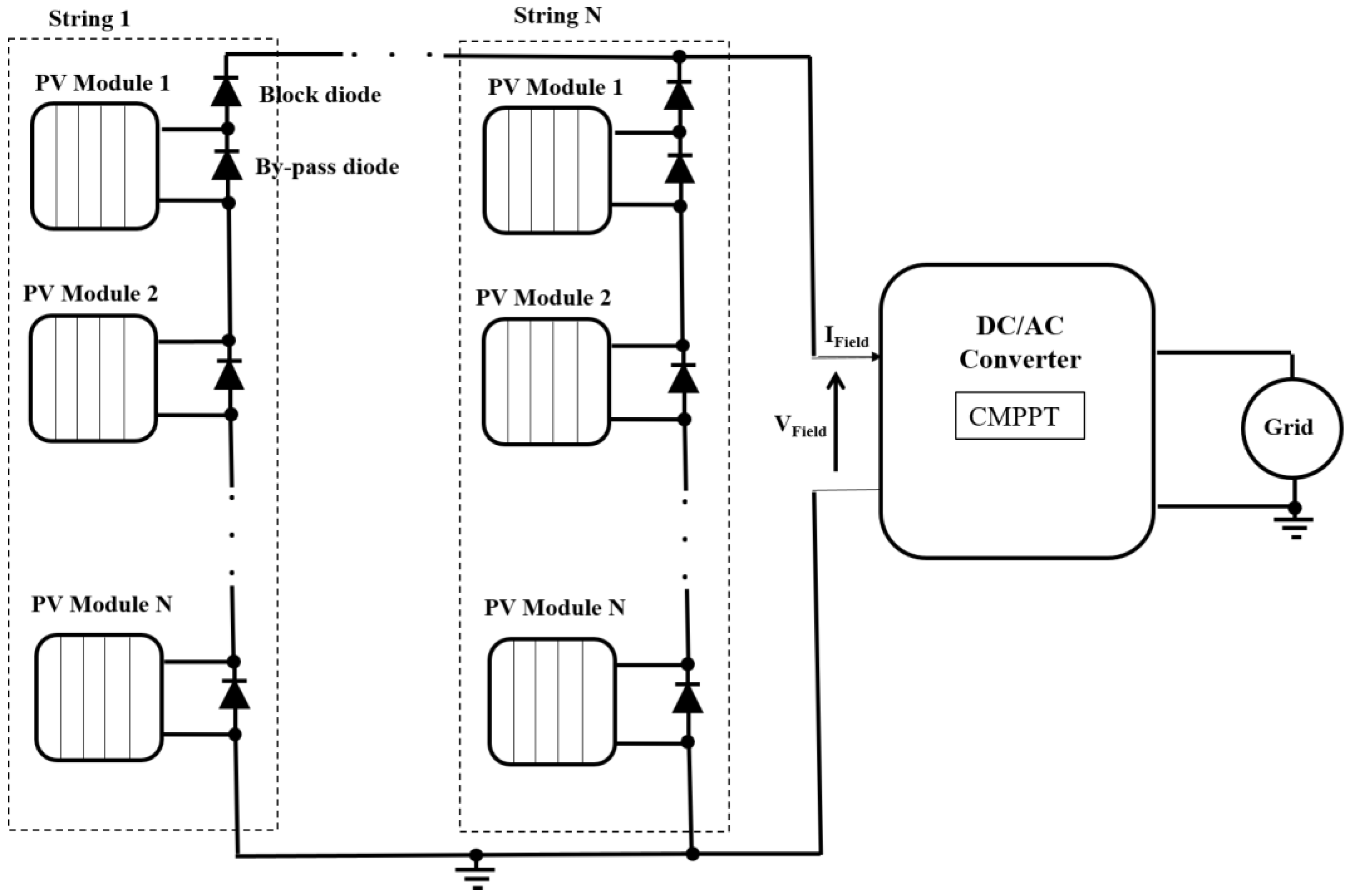
Additionally, although the power that is extracted at AMPPs is less than the total power available [19], an AMPP is not a feasible point or does not belong to the operating range of the inverter; thus, it is evident, under mismatching conditions, that the centralized approach, which adopts a unique DC/AC converter that carries out the MPPT function of the entire field (Figure 1), cannot guarantee good energy performance. The above approach is known as “Central Maximum Power Point Tracking (CMPPT)”.

A specific tool that can mitigate the above drawbacks associated with mismatched operating conditions is represented by the dynamic reconfiguration of PV modules by means of proper active switches [21,22,23,24,25,26,27,28,29,30,31]. This reconfiguration approach can yield the best compromise between efficiency (power maximization) and reliability (minimization of localized heating phenomena) [29,30,31].

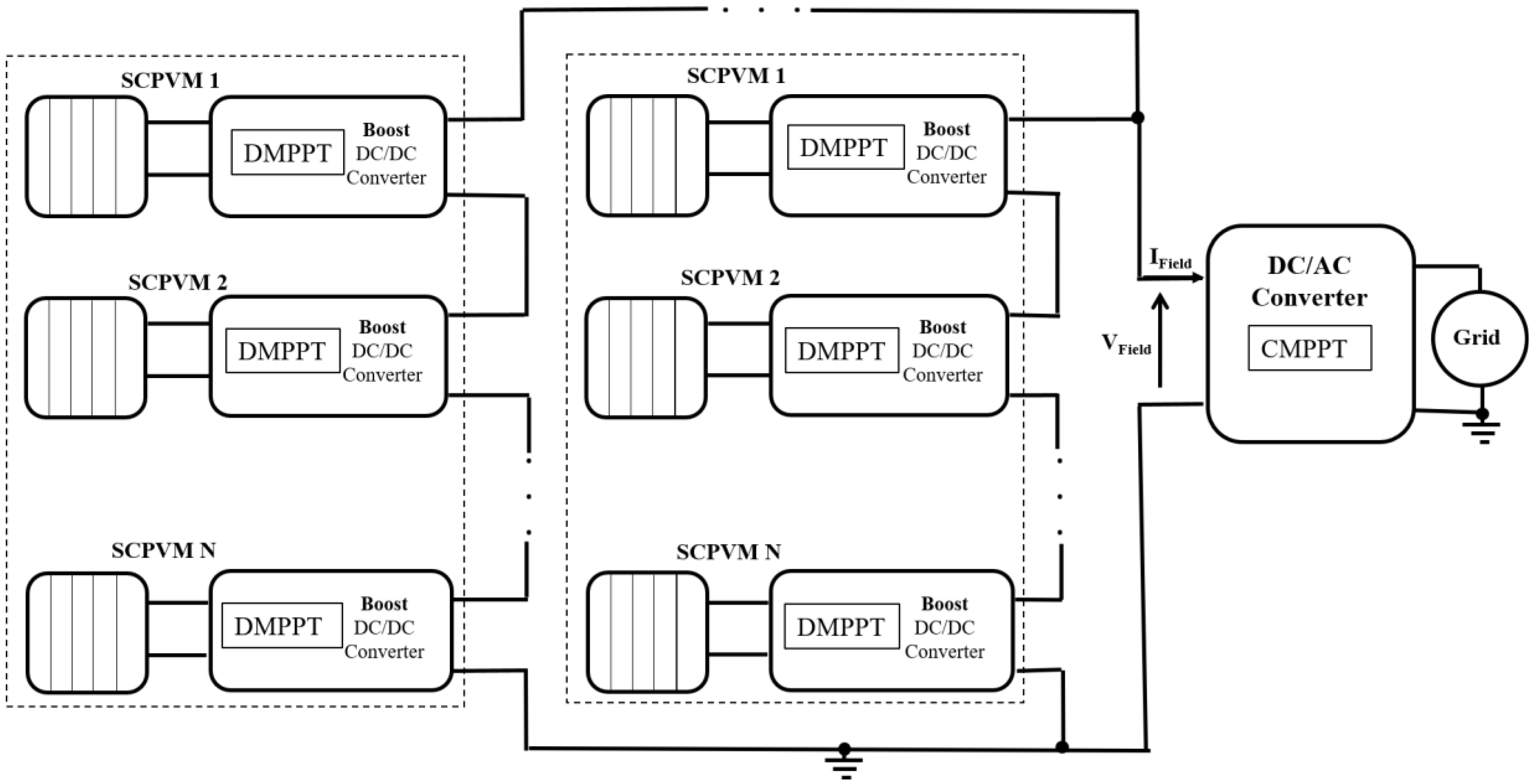
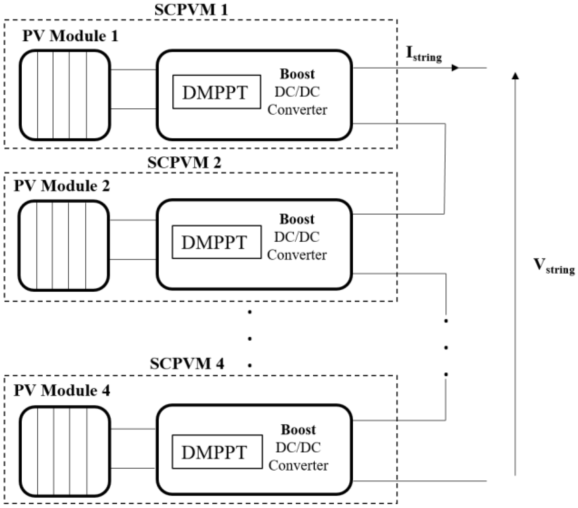
An alternative solution is to use the distributed approach, the classical layout of which is shown schematically in Figure 2 [32,33,34,35,36]. In this case, each PV module is equipped with a DC/DC converter that performs the MPPT function. A system composed of a PV module equipped with a DC/DC converter is called a self-controlled PV module (SCPVM). In particular, SCPVMs, based on the boost topology, are analyzed in this study. Another possibility is to consider SCPVMs based on the buck or buck-boost topology [32,36]. With respect to buck-boost topology, it is characterized by lower efficiencies and higher costs due to enhanced component stresses. In [32,36], such a result has been verified by using the tool represented by the so-called “feasibility region”. In particular, in [32,36], it was shown that a real energy productivity of a buck-boost converter was guaranteed in cases where the mismatch conditions were quite heavy. In all other mismatching scenarios, the buck-boost “feasibility regions” do not include the AMPP, causing a marked reduction of the overall system efficiency. Regarding the buck converter, it optimally works especially in PV systems characterized by a light mismatching scenario, in other words, when, for example, shade or mismatch occurs only on a few PV modules. In this case, the buck DC/DC converter is installed only on those PV modules experiencing shade [32,36]. The adoption of buck converters on all the PV modules of the string is unpractical because of the associated step-down voltage conversion ratio, since it leads to an increase of the number of modules for each string to obtain a string voltage compatible with the input voltage range of the inverter. On the basis of the above assumptions, it is evident that the choice of boost topology provides a less expensive and more reliable solution for distributed maximum power point tracking (DMPPT) applications.

Theoretically, the distributed approach can guarantee maximal efficiency, regardless of the atmospheric conditions and configuration, in terms of electrical connections of SCPVMs. In other words, the efficiency of the entire PV system, as in the case of the centralized approach that works under uniform atmospheric conditions, is related only to the tracking efficiency of the utilized MPPT technique. This aspect is substantially tied to the requirement of ideal conditions, that is, the unit efficiency of the power stage and the total absence of limitations both on the current and on the voltage of the involved silicon devices. In particular, the occurrence of the abovementioned condition (ideal condition) means that the optimal working range is unrestricted, and also that it exhibits a power that coincides with the total available power. These last conditions should hold regardless of the weather conditions and the network topology.

Moving away from these ideal assumptions toward more realistic situations, the energy performance of the distributed approach depends on the power stage efficiency and on the network topology. While the dependence of the distribute approach’s efficiency on the environmental conditions and on the power stage efficiency have been discussed extensively in literature, as highlighted in [31,32,33,34,35], the same discourse cannot be extended to the role assumed by the dynamic reconfiguration of SCPVM-like tools for improving the energy performance of the distributed approach. Until now, reconfiguration techniques and distributed MPPT (DMPPT) have been considered as two alternative techniques. In this work, for the first time, these two methods are combined. In particular, the present work aims to analyze the impact of the joint action of the distributed approach and dynamic reconfiguration in a broader perspective as compared with those closely related to the extracted power.

2. The Current Versus Voltage (I-V) and P-V Characteristics of a Single SCPVM

A few simple guidelines are provided to obtain the current versus voltage (I-V) and the P-V output static characteristics of lossless SCPVM, based on the boost topology. The knowledge of such features represents the starting point for developing the I-V and P-V characteristics of a string, consisting of an arbitrary number of SCPVMs connected in series. The term “lossless” means that, in the ensuing reasoning, the losses occurring in the power stage of the adopted DC/DC converters (switching losses, conduction losses, and iron losses) are neglected. In addition, the MPPT efficiency of the DMPPT controllers is considered to be equal to one. In a follow-up study, the above assumptions will be relaxed. 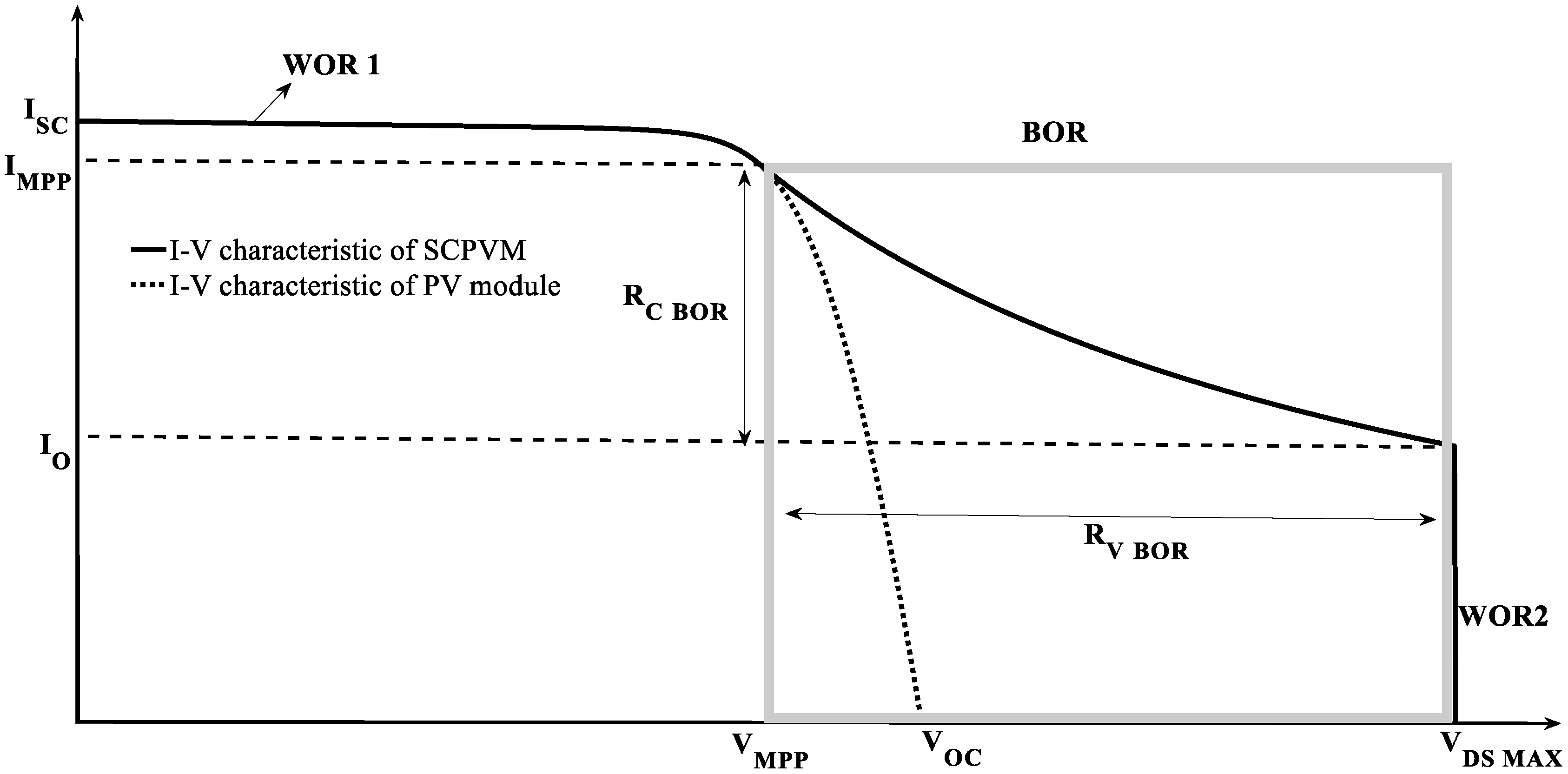In this study, ${\mathrm{V}}_{\mathrm{SCPVM}}$ (${\mathrm{I}}_{\mathrm{SCPVM}}$) denotes the output voltage (current) of the considered SCPVM, and ${\mathrm{V}}_{\mathrm{DSMAX}}$ indicates the maximal allowed voltage provided by the utilized silicon devices. As shown in Figure 3, the I-V characteristic of a single lossless SCPVM is defined by the following three different regions: best operating region (BOR), and two worst operating regions (WOR1 and WOR2). The BOR, defined for ${\mathrm{V}}_{\mathrm{MPP}}\le {\mathrm{V}}_{\mathrm{SCPVM}}<{\mathrm{V}}_{\mathrm{DSMAX}}$, is delimited by the hyperbole of equation ${\mathrm{V}}_{\mathrm{SCPVM}}{\mathrm{I}}_{\mathrm{SCPVM}}={\mathrm{P}}_{\mathrm{MPP}}$, where ${\mathrm{V}}_{\mathrm{MPP}}\left({\mathrm{P}}_{\mathrm{MPP}}\right)$ is the maximum voltage (power) that can be provided by the adopted PV module under the considered atmospheric conditions (irradiance and ambient temperature) [19,20]. The voltage (${\mathrm{R}}_{\mathrm{V}\mathrm{BOR}}$) and current (${\mathrm{R}}_{\mathrm{C}\mathrm{BOR}}$) ranges associated with the BOR are as follows:

$${\mathrm{R}}_{\mathrm{C}\mathrm{BOR}}=\left]{\mathrm{I}}_0{,\mathrm{I}}_{\mathrm{MPP}}\right]$$

(1)

$${\mathrm{R}}_{\mathrm{V}\mathrm{BOR}}=\left]{\mathrm{V}}_{\mathrm{MPP}}{,\mathrm{V}}_{\mathrm{DSMAX}}\right]$$

(2)

where ${\mathrm{I}}_0$ represents the value of the output current when the output voltage is equal to ${\mathrm{V}}_{\mathrm{DSMAX}}$. Its value is:

$${\mathrm{I}}_0=\frac{{\mathrm{P}}_{\mathrm{MPP}}}{{\mathrm{V}}_{\mathrm{DSMAX}}}$$

(3)

Regarding WOR1, defined for $0\le {\mathrm{V}}_{\mathrm{SCPVM}}<{\mathrm{V}}_{\mathrm{MPP}}$, it is delimited by a portion that coincides with the I-V characteristic of the adopted PV module (dashed line of Figure 3) under the considered atmospheric conditions [19,20]. As shown in Figure 3, WOR 1 can be identified through the following ranges:

$${\mathrm{R}}_{\mathrm{C}\mathrm{WOR}1}=\left]{\mathrm{I}}_{\mathrm{MPP}}{,\mathrm{I}}_{\mathrm{SC}}\right]$$

(4)

$${\mathrm{R}}_{\mathrm{V}\mathrm{WOR}1}=\left[{0,\mathrm{V}}_{\mathrm{MPP}}\right[$$

(5)

where $I_{SC}$ represents the short circuit current of the PV module. At the right-ended limit, WOR2 is characterized by a vertical drop located at $\mathrm{V}={\mathrm{V}}_{\mathrm{DSMAX}}$ and by the action of the output overvoltage protection circuitry. The range of currents associated with WOR 2 is the following one:

$${\mathrm{R}}_{\mathrm{C}\mathrm{WOR}2}=\left[{0,\mathrm{I}}_0\right]$$

(6)

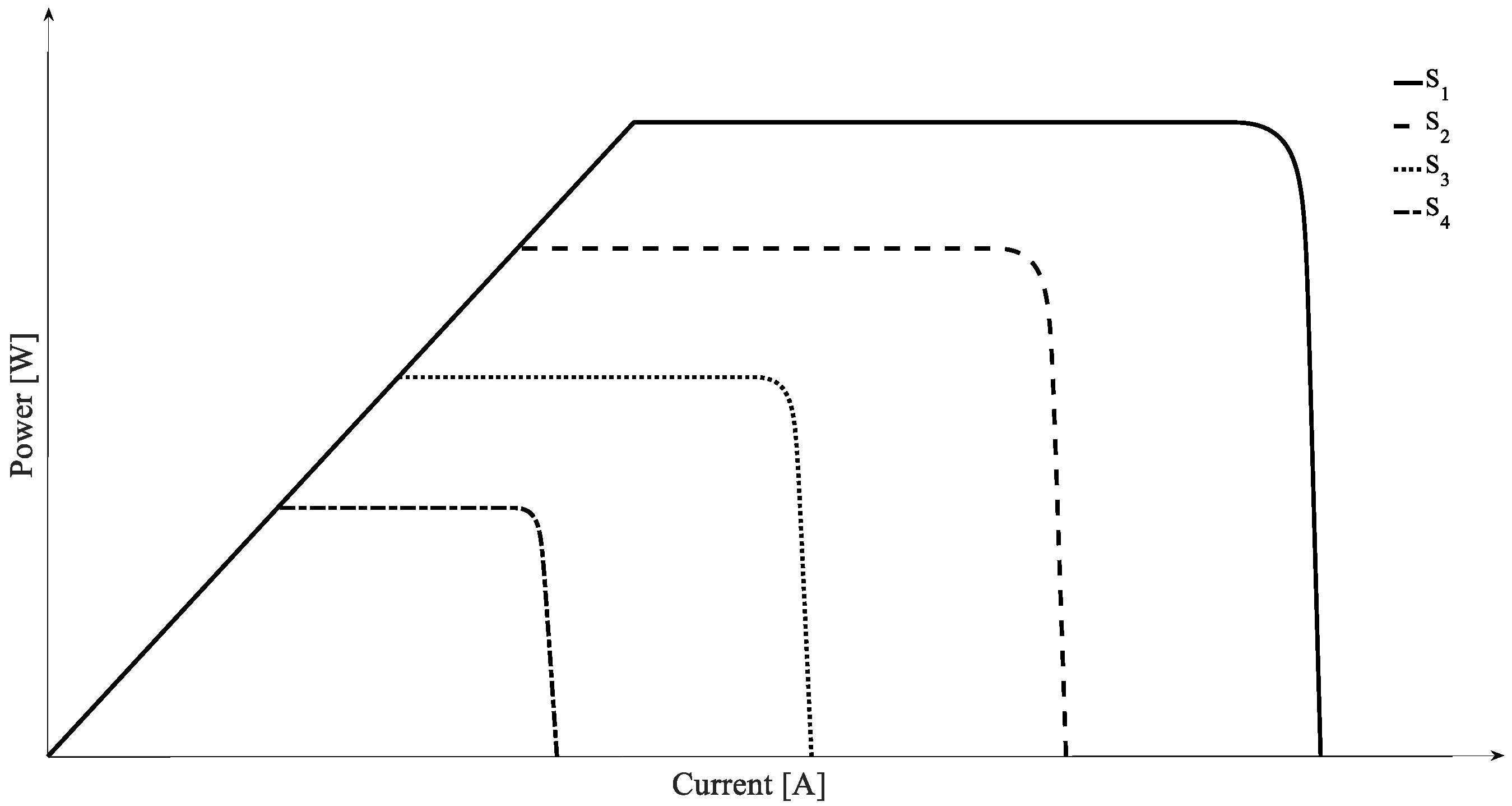
Equations (1) and (2) highlight the propensity of the BOR to assume, under non-stationary operating conditions (S(t), T(t)), time-varying characteristics. This last aspect is crucial in the following reasoning. As an example, Figure 4 shows the power versus current (P-I) characteristics of a single SCPVM obtained by considering four different irradiance values (${\mathrm{S}}_{\mathrm{i}}\mathrm{with}\mathrm{i}=1,\dots ,4$). In particular, the following condition is assumed to be met:

$${\mathrm{S}}_1>{\mathrm{S}}_2>{\mathrm{S}}_3>{\mathrm{S}}_4$$

(7)

3. The Role of the Reconfiguration in DMPPT PV Applications

In the previous section, it was shown that under non-stationary operating conditions, the optimal working interval of a single SCPVM, whether assessed in terms of the current or the voltage, has time-varying characteristics; the latter were attributed not only to their position in the I-V plane, but also to their amplitude (Figure 4). The same considerations, as expected, can be extended to more complex systems, as those shown in Figure 2, which consist of many strings of SCPVMs connected in parallel. Evidently, once this property is confirmed, there is a need to continuously converge the work-point to be within that range. The need for the joint action between centralized and distributed control, given the characteristic time variation of the optimal work range, is well assessed, as can be seen in [19,20]. This approach is known as hybrid maximum power point tracking (HMPPT). The hybrid approach is the most effective solution for overcoming the highlighted limits of the distributed approach. However, there are working conditions under which, even for the hybrid approach, the efficiency of the entire system is strongly weakened. When the critical aspects of the distributed approach against the reliability of DC/DC converters and PV panels are considered, in addition to the aspect of energy performance, in terms of the power extracted, it becomes clear that the impaired quantity is the energy that is produced during the entire useful life of the PV plant itself.

To better understand the above concepts, in the following it is considered appropriate, first of all, to refer to a PV system with a simple topology, and then to extend the results to more complex systems. In particular, at first a PV system consisting of a single string of N_S = 4 SCPVMs (SCPVM1, SCPVM2, …, SCPVM4) is considered. The decision to analyze a system of only four SCPVMs connected in series arises from the need to identify a configuration that is easy to be resolved but, at the same time, considers all the previously highlighted arguments. The most scrutinized aspect is the role assumed by a particular network topology on the energy performance of the entire system. In other words, we show how the critical issues affecting the distributed approach are overcome, both partially and totally, by acting on the configuration [36]. In particular, the authors want to highlight the idea that the distributed approach and reconfiguration techniques, which up to now have been considered as alternative techniques, are actually complementary.

To better understand the exposed aspects, the tested system (shown in Figure 5), is analyzed for three specific cases which correspond to three different working conditions (Cases A, B, and C). Each of the above cases refers to a set of possible mismatching conditions to which a PV system can be subjected. The objective is to obtain results that are representative of the various combinations of possible mismatching scenarios (Figure 6). Cases A and B represent, respectively, the best and the worst cases whereas, as depicted in Figure 6, Case C is the relative complement of the various combinations of possible mismatching scenarios with respect to the union of Case A and Case B. As a consequence, for exhaustive analysis, it is necessary to analyze only the first two of the three envisaged cases. It is important to clarify for the reasoning that follows, that no reference to atmospheric quantities (e.g., irradiance and temperature) is considered, and only the electrical quantities directly or indirectly connected to them (such as $I_{SC}, I_{MPP}, I_0, and V_{MPP}$) are considered. This approach, which seems like a limitation, is in fact quite realistic as it defines the electrical properties (in terms of voltage and current) that must be satisfied by a string in order to improve the energy performance. Moreover, with the aim of obtaining results with general validity, no reference to numerical values is made.

3.1. Case A: Best Case

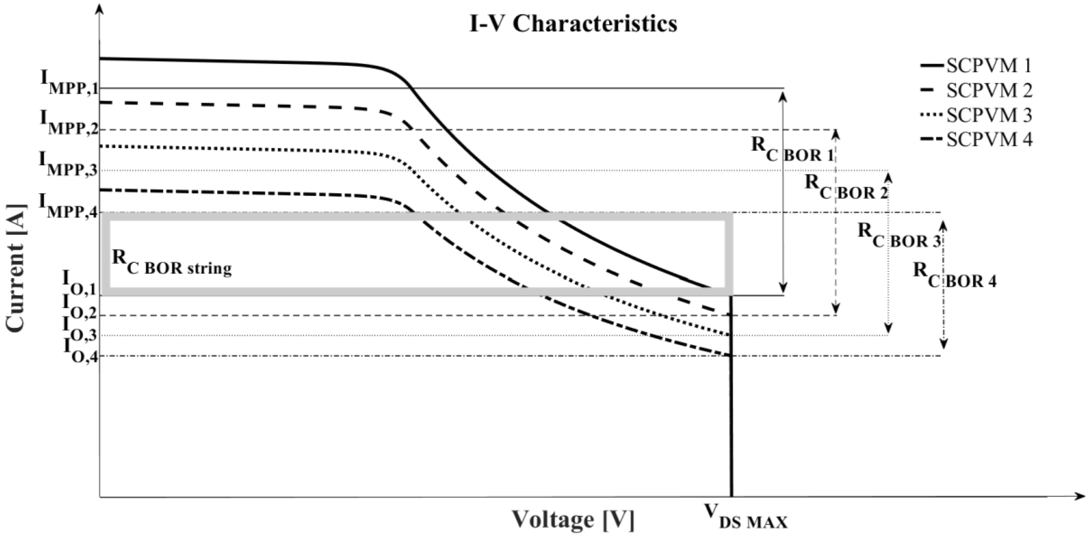
Case A refers to the I-V curves shown in Figure 7. This figure, in addition to showing the I-V characteristics of each individual SCPVM, also highlights the respective optimal working current ranges ($R_{C BOR,i}$ with I = 1, 2, 3, and 4). Moreover, the following condition is assumed:

$$I_{MPP,i}>I_{MPP,j}\left(ifi>j\right)$$

(8)

The opposite occurs regarding the temperatures and the respective voltages at the MPP points. Another condition to be verified, always with respect to what is shown in Figure 7, is the following:

$$I_{0,1}<I_{MPP,4}<I_{MPP,1}$$

(9)

The above condition, as expected, represents the necessary and sufficient condition for not only having an intersection between the optimal current ranges of all SCPVMs, but also that such an intersection yields the optimal current range of the entire string ($R{C}_{BOR string}$). Thus:

$${\mathrm{R}}_{\mathrm{C}\mathrm{BOR}\mathrm{string}}={\mathrm{R}}_{\mathrm{C}\mathrm{BOR}1}{\displaystyle \cap }{\mathrm{R}}_{\mathrm{C}\mathrm{BOR}2}\dots \dots {\displaystyle \cap }{\mathrm{R}}_{\mathrm{C}\mathrm{BOR}4}=\left]{\mathrm{I}}_{0,1}{,\mathrm{I}}_{\mathrm{MPP},4}\right]$$

(10)

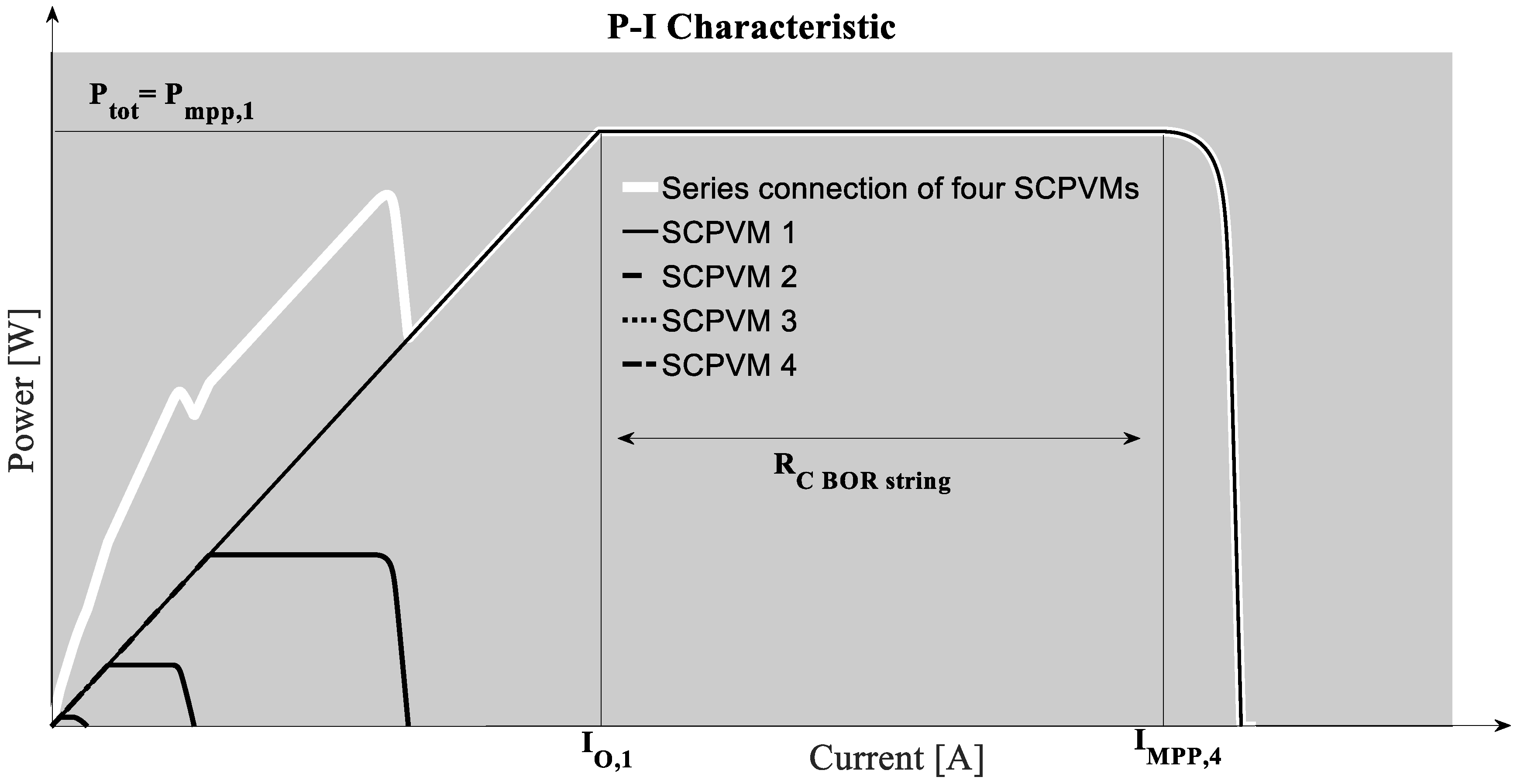
The particular link highlighted by Equation (10), which relates the optimal range of the working current of the entire string to those of individual SCPVMs, clearly denotes its predisposition to assume, under mismatching and not-stationary conditions, time-varying characteristics. Apart from this aspect which, as explained above, does not provide any innovative contribution, Equation (10) highlights the property according to which all SCPVMs contribute to the definition of the optimal current range of the entire string. This result, from the energy point of view, implies that the optimal working point at which the PV system can deliver the maximum available power, is a feasible point. This statement implies, in all mismatching scenarios, given that Condition (9) is met, that the distributed approach can show its true potential (best case). This becomes even more evident by analyzing the P-I characteristic of the entire string (white curves) reported in Figure 8; this characteristic is obtained by adding, for every value of the string current $I_{string}$, belonging to the range $\left[0, I_{SC,1}\right]$, the maximum power values of individual SCPVMs, at the said value of current.

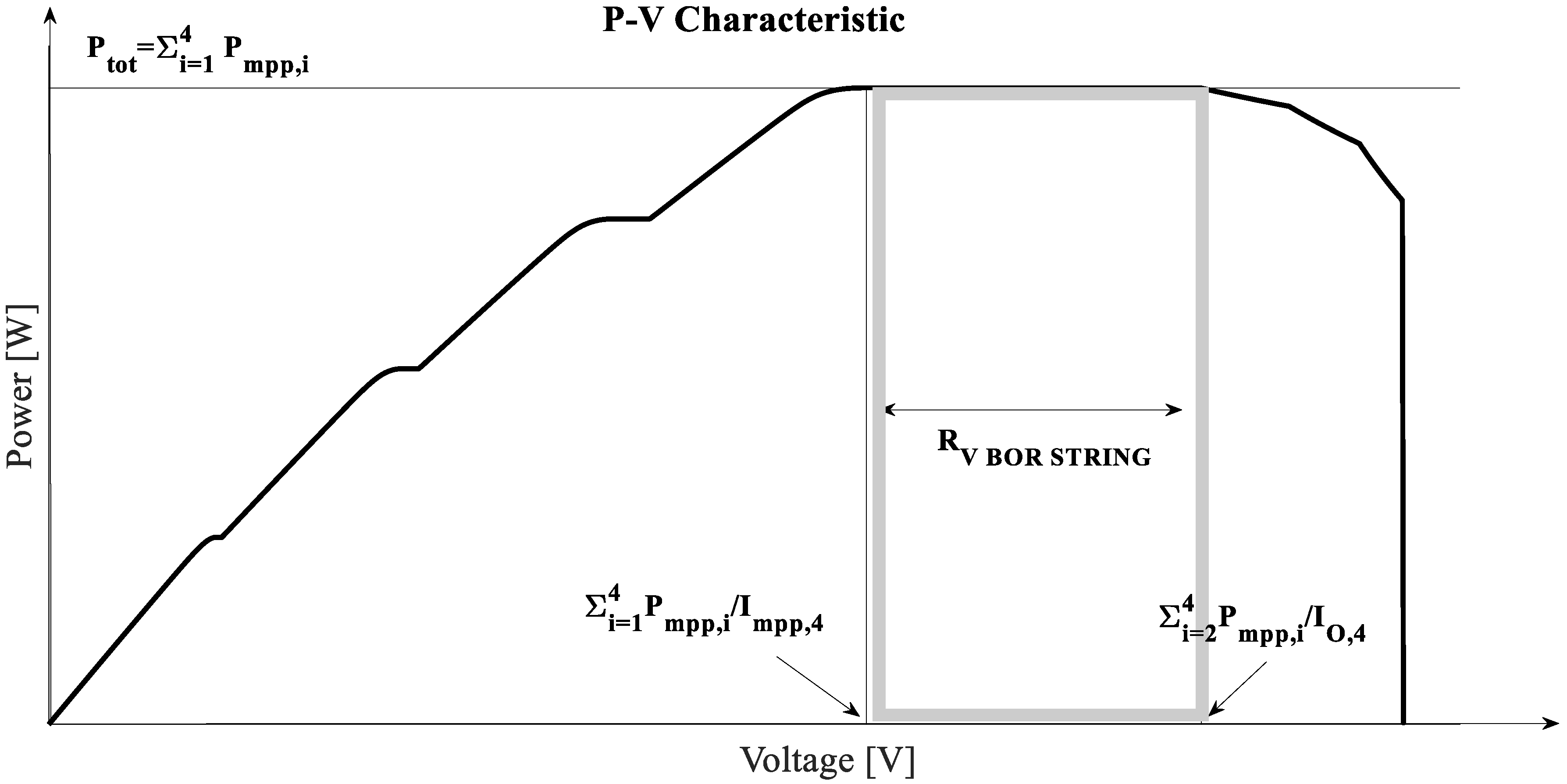
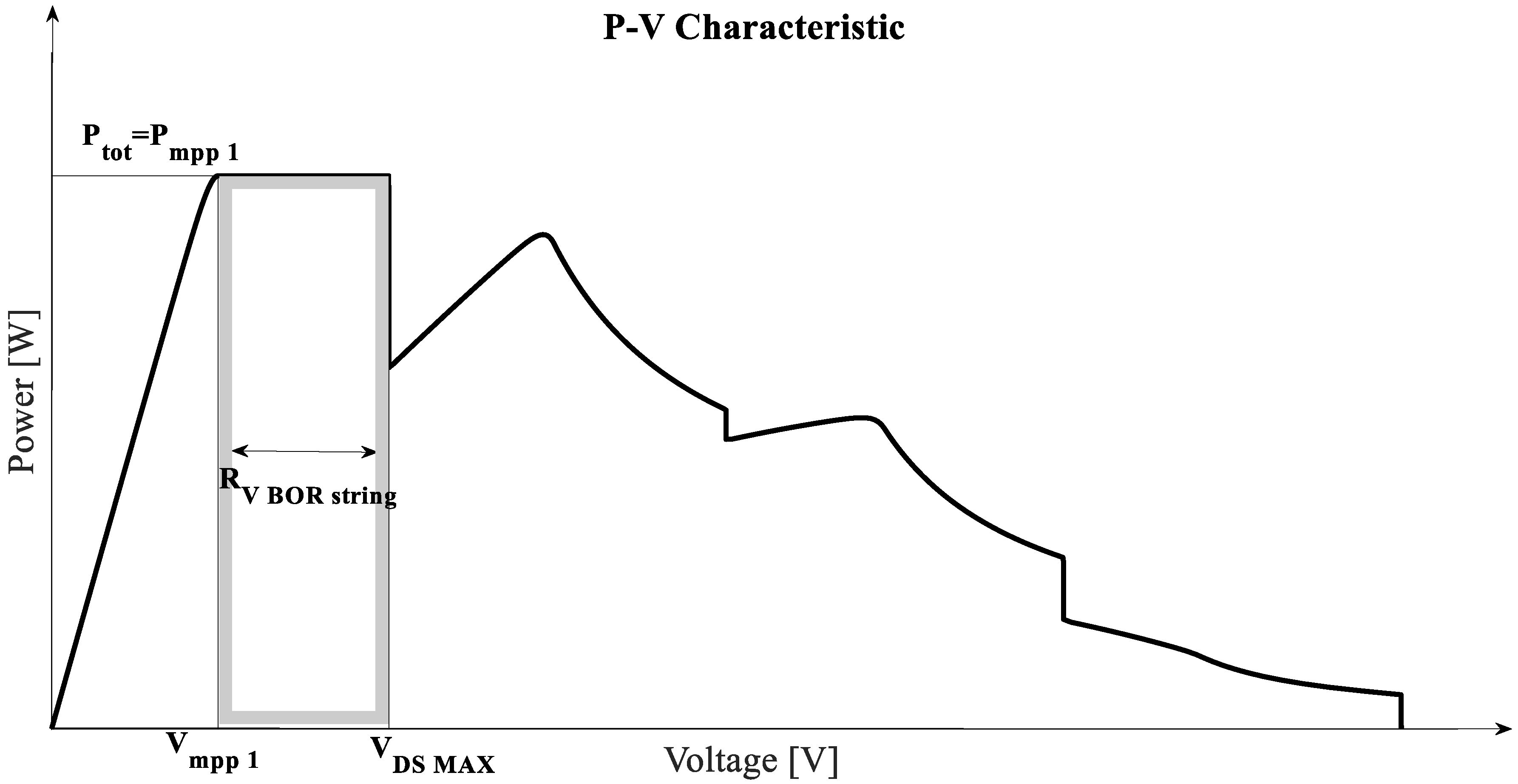
In particular, Figure 8 shows that the optimal working range defines a region where the P-I characteristics of all SCPVMs show a flat shape. Figure 9, for completeness of reasoning, replots the P-V characteristic of the entire system under test, in which the optimal operating voltage range (R_{V BOR string}) of the entire string is evidenced. As expected, the optimal voltage range of the entire system can be expressed not only as a function of the overall available power, but also as a function of the optimal current range. In particular:

$${\mathrm{R}}_{\mathrm{V}\mathrm{BOR}\mathrm{string}}=\frac{{{\displaystyle \sum }}_{\mathrm{i}=1}^4{\mathrm{P}}_{\mathrm{MPP},\mathrm{i}}}{{\mathrm{R}}_{\mathrm{C}\mathrm{BOR}\mathrm{string}}}=\left[\frac{{{\displaystyle \sum }}_{\mathrm{i}=1}^4{\mathrm{P}}_{\mathrm{MPP},\mathrm{i}}}{{\mathrm{I}}_{\mathrm{MPP},4}},\frac{{{\displaystyle \sum }}_{\mathrm{i}=1}^4{\mathrm{P}}_{\mathrm{MPP},\mathrm{i}}}{{\mathrm{I}}_{0,1}}\right[$$

(11)

Finally, both the conditions expressed by Condition (9) and the optimal working time of the current, Equation (10), at least in its extremes, depend indirectly on the atmospheric conditions affecting the SCPVMs, with maximum (SCPVM1) and minimum (SCPVM4) sunshine, respectively. The above result is easily extended to more complex systems, such as that represented by a string composed of any number of SCPVMs. For this particular system, the optimal working ranges for both the current and voltage can be expressed as follows:

$${\mathrm{R}}_{\mathrm{C}\mathrm{BOR}\mathrm{string}}={{\displaystyle \cap }}_{\mathrm{i}=1}^{\mathrm{Ns}}{\mathrm{I}}_{\mathrm{C}\mathrm{OPT}\mathrm{i}}=\left]{\mathrm{I}}_{0,\max }{,\mathrm{I}}_{\mathrm{MPP},\min }\right]$$

(12)

$${\mathrm{R}}_{\mathrm{V}\mathrm{BOR}\mathrm{string}}=\frac{{{\displaystyle \sum }}_{\mathrm{i}=1}^{\mathrm{Ns}}{\mathrm{P}}_{\mathrm{MPP},\mathrm{i}}}{{\mathrm{I}}_{\mathrm{C}\mathrm{OPT}\mathrm{string}}}=\left[\frac{{{\displaystyle \sum }}_{\mathrm{i}=1}^{\mathrm{Ns}}{\mathrm{P}}_{\mathrm{MPP},\mathrm{i}}}{{\mathrm{I}}_{\mathrm{MPP},\min }},\frac{{{\displaystyle \sum }}_{\mathrm{i}=1}^{\mathrm{Ns}}{\mathrm{P}}_{\mathrm{MPP},\mathrm{i}}}{{\mathrm{I}}_{0,\max }}\right[$$

(13)

where the footboard min (max) identifies the SCPVM characterized by the minimum (maximum) level of sunlight. As previously stated, Equations (12) and (13) are valid for a specific subset belonging to the entire constellation of all possible mismatching scenarios that affect the tested PV system; a subset that is defined by the occurrence of the following condition:

$$I_{0max}<I_{MPPmin}<I_{MPPmax}$$

(14)

From the reconfiguration point of view, Equations (12) and (13) define the properties that a string must possess for exhibiting good energy performance, regardless of the atmospheric conditions and characteristics of the inverter in terms of the optimal working range (R_{V inverter}). Specifically, Equation (12) establishes that the maximum energy performance of the string can be obtained only when there is an intersection between the optimal intervals in the currents of all the SCPVMs that constitute it. The above condition is not sufficient: the optimal working voltage range of the entire string must also exhibit an intersection with the optimal working range of the inverter. In particular, the following condition applies:

$${\mathrm{R}}_{\mathrm{V}\mathrm{BOR}\mathrm{string}}{\displaystyle \cap }{\mathrm{R}}_{\mathrm{V}\mathrm{inverter}}\ne \mathsf{\varphi }\Rightarrow \left[\frac{{{\displaystyle \sum }}_{\mathrm{i}=1}^{\mathrm{Ns}}{\mathrm{P}}_{\mathrm{MPP},\mathrm{i}}}{{\mathrm{I}}_{\mathrm{MPP},\min }},\frac{{{\displaystyle \sum }}_{\mathrm{i}=1}^{\mathrm{Ns}}{\mathrm{P}}_{\mathrm{MPP},\mathrm{i}}}{{\mathrm{I}}_{0,\max }}\right[{\displaystyle \cap }\left[{\mathrm{V}}_{\mathrm{inverter}\min },{\mathrm{V}}_{\mathrm{inverter}\max }\right]\ne \mathsf{\varphi }$$

(15)

where the symbol V_{inverter min} (V_{inverter max}) indicates the minimum (maximum) value of the input inverter voltage and the symbol $\varphi$ refers to the empty range. This last property, as will be evident later, defines the minimal and maximal number of groups of SCPVMs that can compose a string and ensures that the MPP belongs to the optimal range of the inverter, and therefore is a feasible point.

3.2. Case B: Worst Case

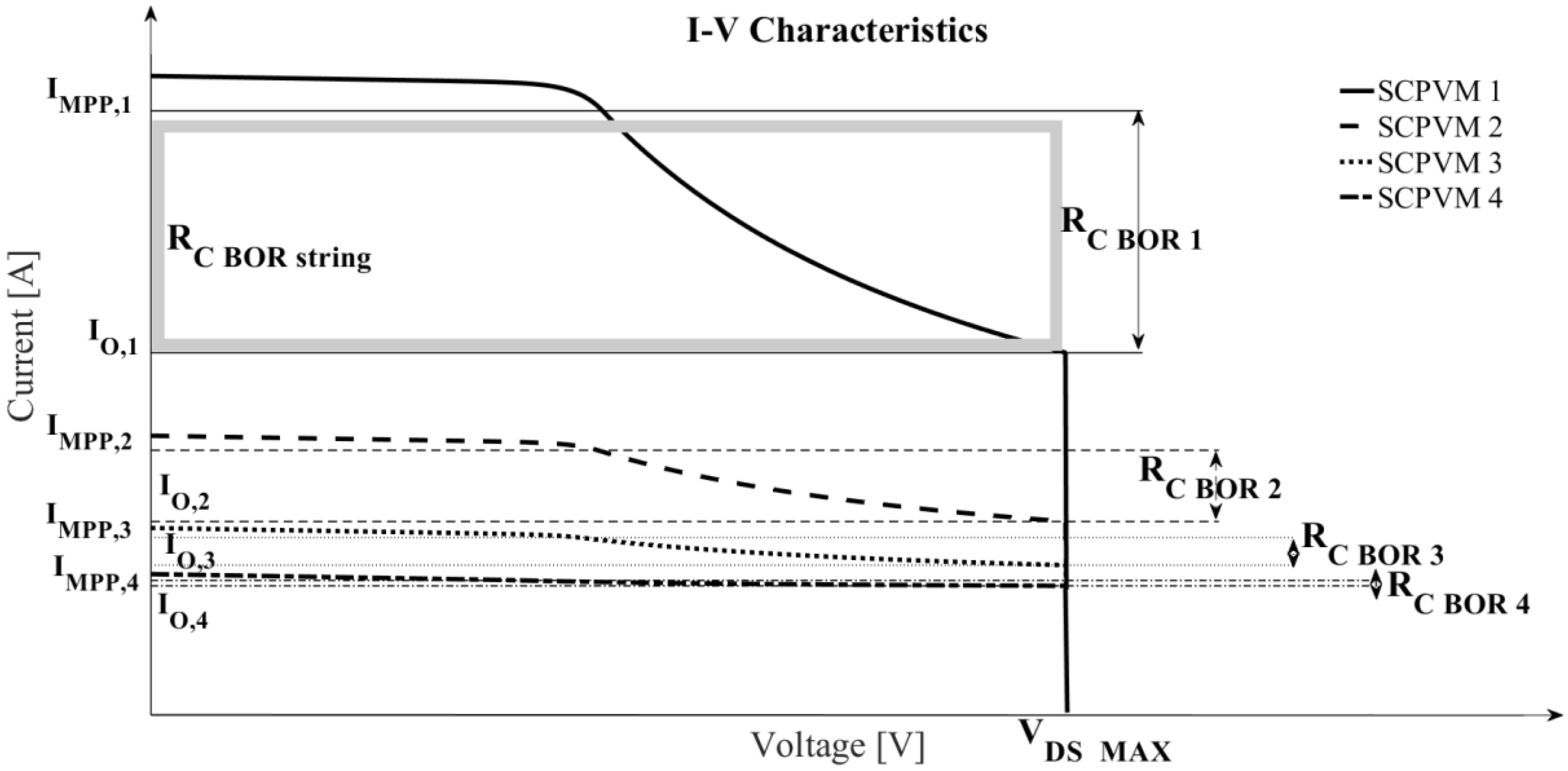
Case B refers to the I-V curves shown in Figure 10, in which, for the sake of clarity, the optimal current ranges of the individual SCPVMs ($R{C}_{BOR\_i}$ with i = 1, 2, 3, and 4) are highlighted. As in Case A, Condition (8) is met ($I_{MPP,i}>I_{MPP,j}$ with $i>j$). The main differences between Case A and Case B relate to the mismatching scenarios; in the present case the following general condition is fulfilled:

$$I_{0,i}>I_{MPP,j}\left(i=1,2,\dots ,N_{S}andj=i+1,i+2,\dots ,N_S\right)$$

(16)

The occurrence of this condition effectively excludes the possibility that there is an intersection between the optimal current intervals of all SCPVMs. As shown in Figure 11, this condition causes the coincidence between $R{C}_{BOR string}$ and $R{C}_{BOR 1}$. The same considerations can be extended with reference to the P-V characteristic plotted in Figure 12, in which it is evident that only SCPVM1 contributes usefully in terms of efficiency to the entire system. Generalizing the above, for all mismatching scenarios that satisfy Condition (16), the optimal range, both in terms of the current and voltage of the entire string, coincides with that of the SCPVM characterized by the maximal level of sunlight (SCPVMmax). That is:

$${\mathrm{R}}_{\mathrm{C}\mathrm{BOR}\mathrm{string}}={\mathrm{R}}_{\mathrm{C}\mathrm{BOR}\max }=\left]{\mathrm{I}}_{0,\max }{,\mathrm{I}}_{\mathrm{MPP},\max }\right]$$

(17)

$${\mathrm{R}}_{\mathrm{V}\mathrm{BOR}\mathrm{string}}={\mathrm{R}}_{\mathrm{V}\mathrm{BOR}\max }=\left[{\mathrm{V}}_{\mathrm{MPP}\max }{,\mathrm{V}}_{\mathrm{DS}\max }\right[$$

(18)

From Equation (17), the limitations of the distributed approach are explicitly evident, with reference to the scenarios described in Case B. At best, the power extractable from the entire PV system coincides with the maximum power delivered by the SCPVM with the highest level of sunlight. In addition to this, if we consider that the pursuit of MPP has occurred at the expense of the reliability of the entire system, it becomes evident that the energy that is produced during the entire useful life of the PV plant is strongly impaired. Moreover, from the analysis of Figure 11, it is useful to point out that the string current belonging to the optimal range ($I_{string OPT}\in R_{\mathrm{C}\mathrm{BOR}\mathrm{string}}$) fulfills the following condition:

$$I_{stringOPT}>I_{SC,i}\left(i=2,3,\dots ,N_S\right)$$

(19)

As a consequence, given the inability of the boost converter to act as active bypass diode [35], it is inevitable that for all those SCPVMs for which Condition (19) is verified, the respective PV modules are reverse biased, and reliability is deeply compromised [37]. Finally, taking into account that the optimal voltage range of the entire string almost certainly falls outside the optimal working range of the inverter, it is evident that the scenarios highlighted by Equations (17) and (18) are not feasible, resulting in a further reduction of efficiency. A solution for limiting these critical issues is to identify a topology that represents the best compromise between efficiency and reliability. For example, a subset of Case B can be considered, such that the following condition is satisfied:

$${\mathrm{I}}_{0\max }<{{\displaystyle \sum }}_{\mathrm{i}=\mathrm{j}}^{\mathrm{Ns}}{\mathrm{I}}_{\mathrm{MPP},\mathrm{i}}\le {\mathrm{I}}_{\mathrm{MPP}\max }\left(\mathrm{j}={2,3,\dots ,\mathrm{N}}_{\mathrm{S}}\right)$$

(20)

In this particular condition, the suitable topology is obtained by the series connection of SCPVMmax with a group of (N_S-j+1) SCPVMs connected in parallel. Moreover, if the possibility, offered by the reconfiguration, of excluding from the entire system the j-2 SCPVMs that do not satisfy Condition (20) is considered, it becomes evident that it is possible to improve the reliability of the entire PV plant by avoiding the presence of PV modules that work in a reverse bias condition. In conclusion, from the above example it is understood that the necessary condition for a string to exhibit good energy performance, regardless the weather conditions, is that there is an intersection between the current optimal ranges of all N_C (Nc $\le$ Ns) groups of SCPVMs that compose it.

Moreover, it is also necessary to guarantee that Condition (15) is satisfied, because the optimal working voltage range of the entire string must also exhibit an intersection with the optimal working range of the inverter. It is necessary that N_C meets the following property:

$$\frac{{\mathrm{V}}_{\mathrm{inverter}\min }}{{\mathrm{V}}_{\mathrm{MPP}}}\le {\mathrm{N}}_{\mathrm{c}}\le \frac{{\mathrm{V}}_{\mathrm{inverter}\max }}{{\mathrm{V}}_{\mathrm{DS}\max }}$$

(21)

The latter property is valid if the following distinction is assumed to be valid:

$$\frac{{\mathrm{V}}_{\mathrm{MPP}}}{{\mathrm{V}}_{\mathrm{DS}\max }}\ge \frac{{\mathrm{V}}_{\mathrm{inverter}\min }}{{\mathrm{V}}_{\mathrm{inverter}\max }}$$

(22)

The minimum number of SCPVMs that belongs to a generic group is equal to one; this implies, in the reasoning that follows, that each individual SCPVM represents a group. Meeting the condition of Property (21) ensures that the optimal working point of the entire string is a feasible point, as it belongs to the operating range of the inverter. Downstream of this brief discussion is a tangible impact of the reconfiguration on the energy performance of PV systems that adopt the distributed approach. The block scheme that jointly involves the distributed approach and the dynamic reconfiguration is shown in Figure 13, in which the presence of the dynamic matrix of switches, located between the PV field and the inverter, is evident. For this system, consisting of Ns SCPVMs distributed on a maximum of N_string strings, the number of switches required is equal to:

$${\mathrm{N}}_{\mathrm{switch}}=4{{\displaystyle \sum }}_{\mathrm{i}=1}^{{\mathrm{N}}_{\mathrm{s}}-1}\left({\mathrm{N}}_{\mathrm{s}}-\mathrm{i}\right)+2\left({\mathrm{N}}_{\mathrm{s}}-1\right){\ast \mathrm{N}}_{\mathrm{string}}$$

(23)

4. Identification of the Best String

In this section, starting from Ns SCPVMs, an algorithm, which determines the string that exhibits the best energy performance is presented and discussed; energy performance here is understood as a compromise between efficiency and reliability. This algorithm is not intended as a reconfiguration algorithm, but rather as a tool for overcoming the belief that the distributed approach and reconfiguration techniques represent alternative solutions to mitigate the effects of the occurrence of mismatching operating conditions. In other words, the purpose of the following discussion is to develop innovative reconfiguration techniques suitable for distributed applications. From the previous paragraph, the necessary condition for a string to exhibit good energy performance, regardless the atmospheric conditions, is that there will be an intersection between the current optimal ranges of all N_C groups of SCPVMs that compose it. That is to say:

$${\mathrm{R}}_{\mathrm{C}\mathrm{BOR}\mathrm{i}}{\displaystyle \cap }{\mathrm{R}}_{\mathrm{C}\mathrm{BOR}\mathrm{j}}\ne \mathsf{\varphi }\left(\mathrm{i}=1,2,\dots {,\mathrm{N}}_{\mathrm{c}}\mathrm{and}\mathrm{j}=\mathrm{i}+1,\mathrm{i}+2,\dots {,\mathrm{N}}_{\mathrm{c}}\right).$$

(24)

According to Property (21), the minimum (N_c min) and maximum (N_c max) values of N_C are defined as follow:

$${\mathrm{N}}_{\mathrm{c}\min }=\frac{{\mathrm{V}}_{\mathrm{inverter}\min }}{{\mathrm{V}}_{\mathrm{MPP}}}$$

(25)

$${\mathrm{N}}_{\mathrm{c}\max }=\frac{{\mathrm{V}}_{\mathrm{inverter}\max }}{{\mathrm{V}}_{\mathrm{SD}\max }}$$

(26)

With the aim of identifying, starting from a number of SCPVMs, the string that fulfills the properties expressed in Equations (24), (25), and (26), the algorithm, object of this paragraph, bases its principle of functioning on an iterative process. The starting point is the definition of the intersection matrix (${\mathrm{I}}_{\mathrm{matrix}}$), defined as follows:

$${\mathrm{I}}_{\mathrm{matrix}}\left(\mathrm{i},\mathrm{j}\right)=\{\begin{array}{cc}1& \mathrm{if}\left({\mathrm{R}}_{\mathrm{C}\mathrm{BOR},\mathrm{i}}{\displaystyle \cap }{\mathrm{R}}_{\mathrm{C}\mathrm{BOR},\mathrm{j}}\ne \mathsf{\varphi }\right)\\ 0& \mathrm{if}\left({\mathrm{R}}_{\mathrm{C}\mathrm{BOR},\mathrm{i}}{\displaystyle \cap }{\mathrm{R}}_{\mathrm{C}\mathrm{BOR},\mathrm{j}}=\mathsf{\varphi }\right)\end{array}$$

(27)

where $\mathrm{i}=1,2,\dots {,\mathrm{N}}_{\mathrm{s}};\mathrm{and}\mathrm{j}=\mathrm{i}+1,\mathrm{i}+2,\dots {,\mathrm{N}}_{\mathrm{s}}.$

Under the hypothesis that the level of sunlight decreases with increasing the footboard (${\mathrm{I}}_{\mathrm{MPP},\mathrm{i}}>{\mathrm{I}}_{\mathrm{MPP},\mathrm{j}}\left(\mathrm{if}\mathrm{i}>\mathrm{j}\right)$), at each row of ${\mathrm{I}}_{\mathrm{matrix}}$ it is possible to associate a cluster, which is called an optimal cluster (OC), composed of all SCPVMs accomplishing ownership in Condition (24). Since I_matrix is an [N_S ×N_S] matrix, the number of OCs that can be associated with ${\mathrm{I}}_{\mathrm{matrix}}$ is N_S (the number of rows of I_matrix). For the sake of clarity, in the following, we indicate by OCi the optimal cluster associated with the i-th row of ${\mathrm{I}}_{\mathrm{matrix}}$. In addition, we denote by NC_i and R_{C OPT OCi}, respectively, the number of groups of SCPVMs belonging to the i-th cluster (OC_i) and the optimal current interval, obtained by connecting in series all the N_Ci SCPVMs belonging to OC_i. According to the value assumed by N_Ci, compared with the overall number of SCPVMs (N_S) that make up the entire PV field, it is possible to discriminate, for each single OC, three potential working conditions: (1) the best condition (N_Ci = N_S), (2) the worst condition (N_Ci = 1), and (3) the compromise condition (1 < N_Ci < N_S). The best case can be neglected because no reconfiguration is necessary; for the other two cases, it is possible to associate with I_matrix additional N_S clusters, each of which is composed of N_S-N_Ci SCPVMs. In other words, the i-th row of I_matrix, in addition to OC_i, can be associated with an additional cluster composed of all SCPVMs which, owing to their characteristics, cannot belong to the corresponding heading. This additional cluster is denoted as the relative complement of i-th optimal cluster (RCOC_i). The number of items belonging to the i-th RCOC is:

$${\mathrm{N}}_{\mathrm{RCOC}\mathrm{i}}={\mathrm{N}}_{\mathrm{S}}-{\mathrm{N}}_{\mathrm{Ci}}\ge 0$$

(28)

On the basis of the above, it is clear that for reasons strictly related to reliability, RCOC_i represents the entire set of the SCPVMs to be excluded, potentially, from the entire PV plant, to avoid the presence of one or more PV modules working in reverse bias conditions. ”Potentially” means that the N_RCOCi SCPVMs have to be excluded only if the following condition is not verified:

$${{\displaystyle \sum }}_{\mathrm{k}=1}^{{\mathrm{N}}_{\mathrm{SCPVM}\mathrm{j}}}{\mathrm{R}}_{\mathrm{C}\mathrm{BOR}\mathrm{subset}\mathrm{k}}{\displaystyle \cap }{\mathrm{R}}_{\mathrm{C}\mathrm{BOR}\mathrm{OC}\mathrm{i}}\ne \mathsf{\varphi }\left(\mathrm{j}={1,2,\dots ,\mathrm{N}}_{\mathrm{subset}\mathrm{i}}\right)$$

(29)

where N_{SCPVM j} indicates the number of SCPVMs belonging to the j-th subset of RCOC_i and N_{subset i}, with the total number of possible subsets belonging to RCOC_i equal to:

$${\mathrm{N}}_{\mathrm{subset}\mathrm{i}}={{\displaystyle \sum }}_{\mathrm{k}=2}^{{\mathrm{N}}_{\mathrm{RCOC}\mathrm{i}}}\frac{{\mathrm{N}}_{\mathrm{RCOCi}}!}{\mathrm{k}!\left({\mathrm{N}}_{\mathrm{RCOCi}}-\mathrm{k}\right)!}$$

(30)

In particular, the occurrence of Condition (29) implies the existence of groups of SCPVMs, whose connection in parallel is such as to exhibit an equivalent optimal current interval (R_{C BOR subset k}) that satisfies Condition (24). Excluding the above groups from RCOC_i and inserting them in OC_i creates the following two new clusters: BC_i (best cluster) and CE_i (cluster of excluded). BC_i represents the extension of OC_i obtained by including groups of SCPVMs, placed in parallel, that satisfy Condition (24). As far as CE_i is concerned, it is clear that, being composed of SCPVMs that do not individually or in groups meet Conditions (24) and (29), it represents the entire set of SCPVMs to be excluded for safeguarding the reliability of the entire plant. Thus, it is concluded that the information contained in BC_i and CE_i identifies the string that satisfies Condition (24). Once the aforementioned clusters are defined, the iterative process on which the algorithm is based ends identifying, between the possible N_S strings, the one which not only meets the Conditions (25) and (26) but is also characterized by the maximum extracted power. This string represents, as can be expected, the best compromise between efficiency and reliability.

In the following, as an example, the results obtained using the above algorithm are considered with reference to two different mismatching scenarios, i.e., Case I and Case II. In both cases, the tested PV system is characterized by the presence of N_S = 4 SCPVMs, whose electrical characteristics are listed in

Table 1. Electrical characteristics of the SCPVMs.

Open Circuit Voltage (Standard Test Conditions)	VOC_STC = 37.3 V
Short Circuit Current (Standard Test Conditions)	ISC_STC = 8.13 A
Maximum Power Point Voltage (Standard Test Conditions)	VMPP_STC = 29.7 V
Maximum Power Point Current (Standard Test Conditions)	IMPP_STC = 7.59 A
Maximum Allowed Voltage (Standard Test Conditions)	VDS MAX = 60 V

, which indicates the clear reference to commercial PV panels (SW 225 of Solar World) [38]. As far as the inverter is concerned, it is assumed that it is characterized by an operating range whose input values are shown in

Table 2. Input inverter range.

Minimum Inverter Voltage	60 V
Maximum Inverter Voltage	240 V

.

Replacing the values in Table 1 and Table 2 by Equations (25) and (26), the minimal and maximal number of groups of SCPVMs for ensuring that the optimal voltage range of the entire range is contained in the optimal operating range of the inverter is equal to:

$${\mathrm{N}}_{\mathrm{cmin}}=\frac{{\mathrm{V}}_{\mathrm{inverter}\min }}{{\mathrm{V}}_{\mathrm{MPP}\_\mathrm{STC}}}\cong 2$$

(31)

$${\mathrm{N}}_{\mathrm{cmax}}=\frac{{\mathrm{V}}_{\mathrm{inverter}\max }}{{\mathrm{V}}_{\mathrm{DS}\max }}\cong 4$$

(32)

4.1. CASE I

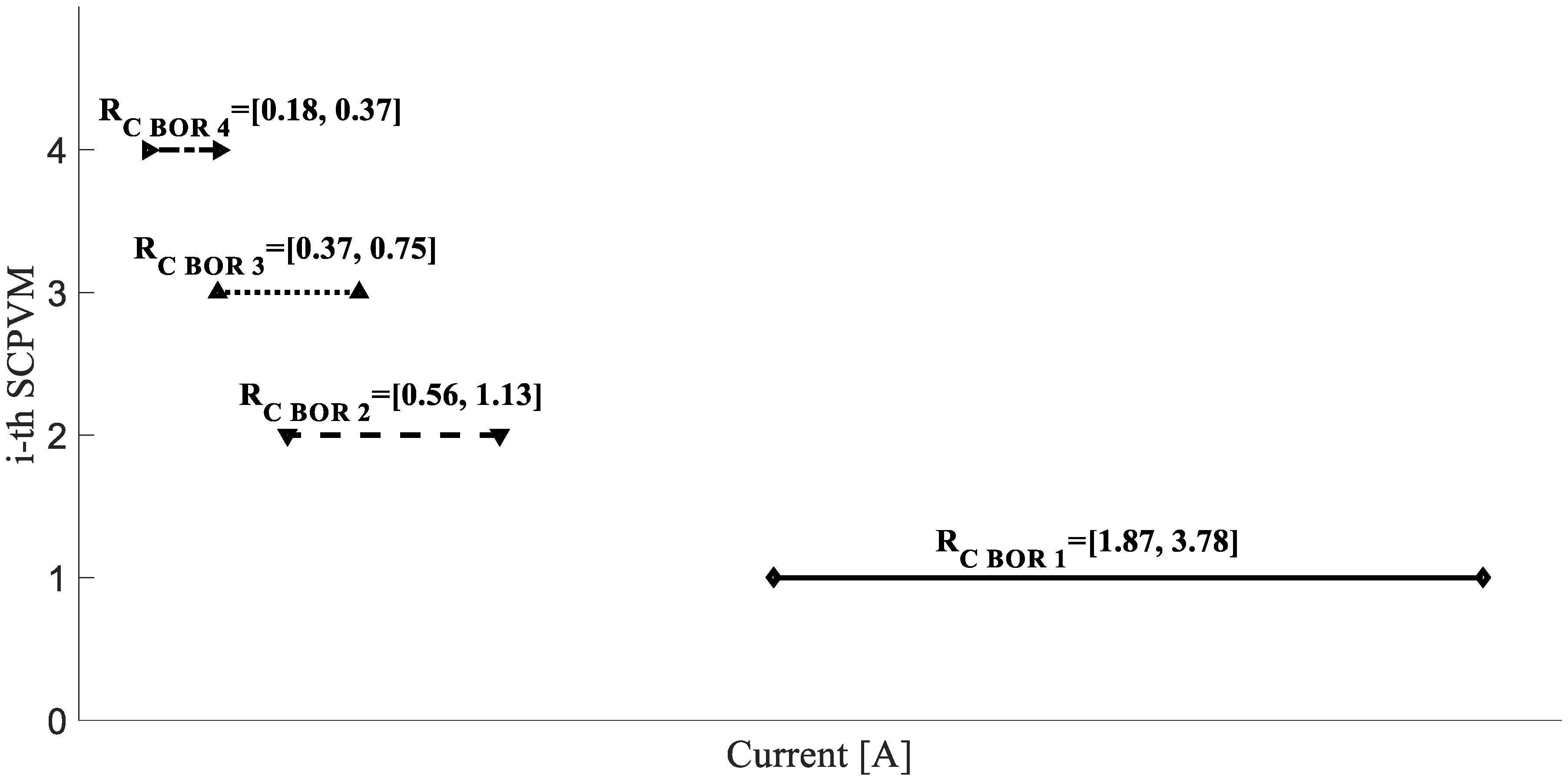
Case I refers to the following set of values: I_MPP vector I_{MPP_V} = [3.78 1.13 0.75 0.37] A, I₀ vector I_{0_V} = [1.87 0.56 0.37 0.18] A. Figure 14 shows the optimal current ranges of all SCPVMs.

With reference to Case 1, the matrix of intersections, obtained by applying the conditions expressed in Equation (27), is as follows:

$${\mathrm{I}}_{\mathrm{matrix}}=\left(\begin{array}{c}1000\\ 0110\\ 0011\\ 0001\end{array}\right)$$

(33)

Row 1: From the intersection matrix it is evident that the first line has only one non-zero element in the I_matrix position (1,1). This implies that the intersection of the optimal current range of the SCPVM₁ with all the remaining SCPVMs is empty. Therefore, the set OC₁ consists of a single group made up of SCPVM₁ (NC₁ = 1) while SCPVMs 2, 3, and 4 belong to RCOC₁ (N_RCOC1 = 3) by exclusion. The presence of N_RCOC1 = 3 SCPVMs inside RCOC₁ implies the existence of four possible subsets, each consisting of the parallel of a minimum of two up to a maximum of three SCPVMs.

Table 3. Subsets associated with relative complement of i-th optimal cluster (RCOC1).

Description	Group	Optimal Current Range
Subset 1	SCPVM2//3	[0.93, 1.88] A
Subset 2	SCPVM2//4	[0.74, 1.5] A
Subset 3	SCPVM3//4	[0.55, 1.12] A
Subset 4	SCPVM2//3//4	[1.11, 2.25] A

shows the compositions of each single group together with their optimal current range. For simplicity “i//j” denotes the group constituted by the parallel connection of i-th SCPVM with j-th SCPVM. A comparison of the intervals represented in Table 2 with the optimal range associated with OC₁ which coincides with that of SCPVM₁, shows that only Subsets 1 and 4 satisfy Equation (29). Of the above subsets, Subset 4 is more suitable as it is associated with a greater extractable power being constituted by the parallel connection of three SCPVMs. On the basis of the above, it is clear that cluster CE₁, associated with the first row of I_matrix, is empty, while cluster BC₁ consists of two groups composed, respectively, of SCPVM₁ and the parallel connection of SCPVM 2, 3, and 4 (SCPVM _2//3//4).

Rows 2, 3, 4: Repeating the process also for Rows 2, 3 and 4 it is possible to obtain the results shown in

Table 4. Best clusters (BCs) and clusters of excluded (CEs) (Case I).

Row	BC	CE	Pav
1	SCPVM1; SCPVM2//3//4	ϕ	176.5 W
2	SCPVM2; SCPVM3	SCPVM1; SCPVM4	56.25 W
3	SCPVM3; SCPVM4	SCPVM1; SCPVM2	33.75 W
4	SCPVM4	SCPVM1; SCPVM2; SCPVM3	11.25 W

.

From the analysis of Table 4, it is easy to identify the string that most of all represents the best compromise between efficiency and reliability, which in the case under consideration is obtained by connecting in series the groups belonging to BC₁. This statement is reflected in the fact that groups belonging to BC₁ not only meet Condition (21) but are capable, once connected in series, to display a greater (P_av = 176.5 W) available power than the strings obtained by connecting in series the groups belonging to other BC_i (with i = 2, 3, and 4). 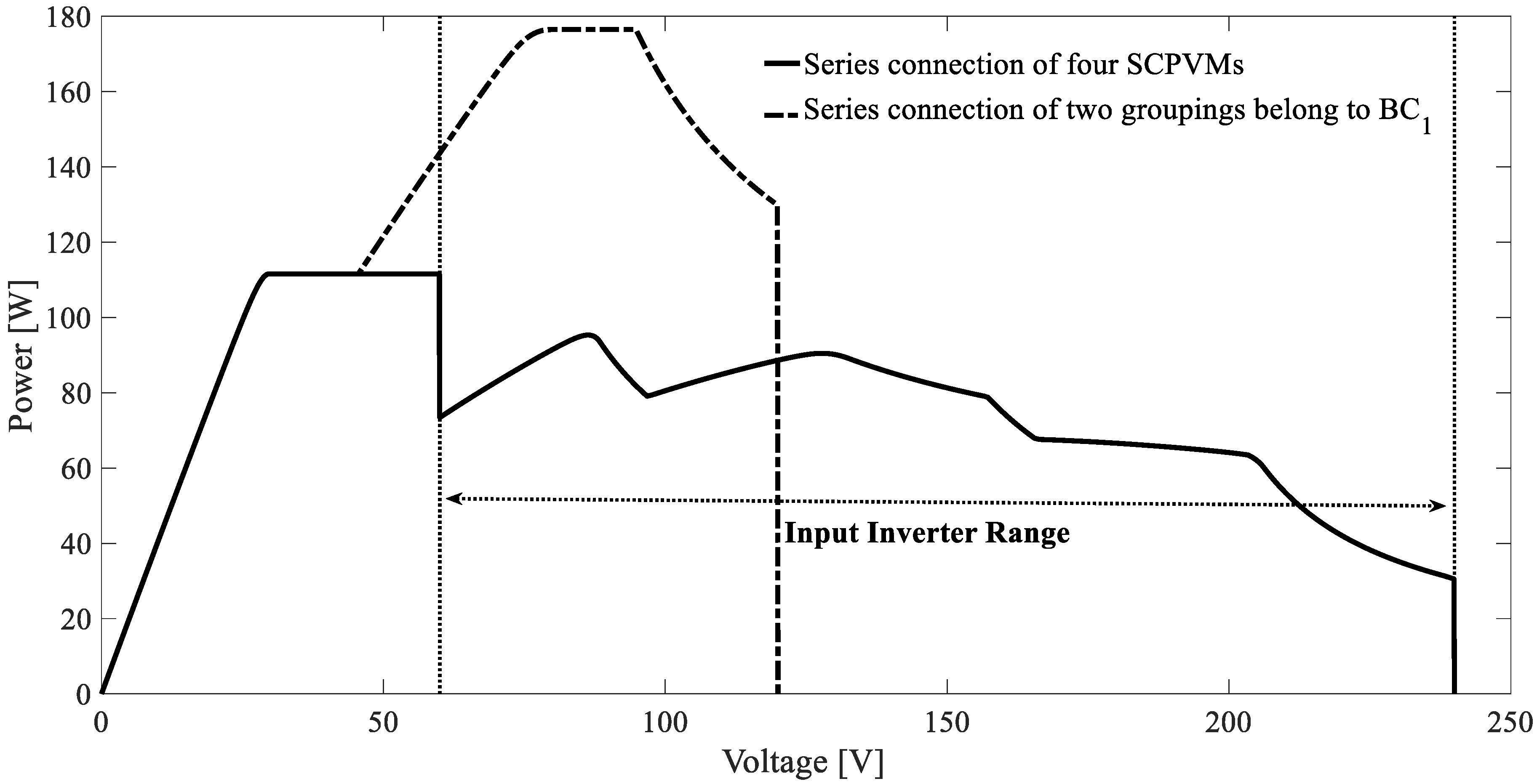To further highlight the results obtained using this algorithm, Figure 15 shows the comparison of the P-V characteristics of the string just identified (continuous line) with that obtained by connecting in series all the four SCPVMs (dotted line). From Figure 15, we perceive an evident increase of the extractable power inside the operating range of the inverter, estimated as ~85%. The increased extractable power is not the only advantage of using an appropriate reconfiguration of SCPVMs, which in the present case is obtained through the series connection of groups belonging to BC₁. In particular, unlike the string obtained from the series connection of the four SCPVMs, the presence of SCPVMs working under reverse bias conditions has been avoided, at least in the optimal working range, with clear advantages in terms of the reliability of the entire system.

4.2. CASE II

Case II refers to the following set of values: I_MPP vector I_{MPP_V} = [3.03 2.65 1.13 0.75] A, I₀ vector I_{0_V} = [1.5 1.31 0.56 0.37] A.

$$I_{matrix}=\left(\begin{array}{c}1100\\ 0100\\ 0011\\ 0001\end{array}\right)$$

(34)

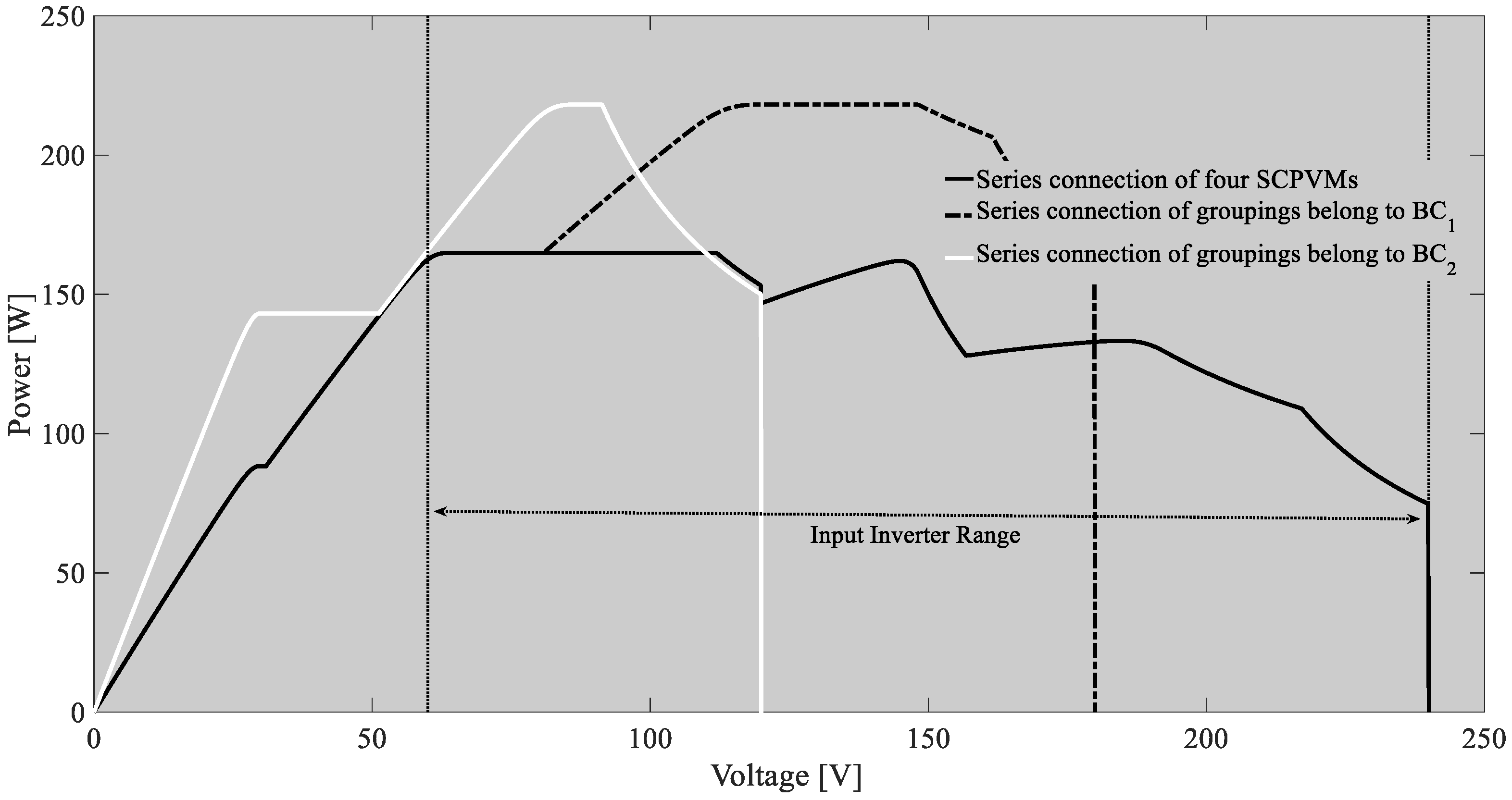
Repeating the reasoning made previously with reference to the case under examination, the obtained results are shown in

Table 5. BCs and CEs (Case II).

Row	BC	CE	Pav
1	SCPVM1; SCPVM2; SCPVM3//4	ϕ	218 W
2	SCPVM2; SCPVM1//3//4	ϕ	218 W
3	SCPVM3; SCPVM4	SCPVM1; SCPVM2	56.25 W
4	SCPVM4	SCPVM1; SCPVM2; SCPVM3	22.5 W

. The presence of two strings that are equivalent from the point of view of the energy performance can be deduced. Again, as shown in Figure 16, the increase in the energy performance with respect to the string, obtained from the series connection of all SCPVMs, is clearly visible and it is estimated as ~32%.

5. Conclusions

This work highlighted the main advantages of a joint action of DMPPT and reconfiguration approaches. Combining the two approaches not only positively affects the energy efficiency, but also increases the reliability of the mismatched PV system. These results suggest that the DMPPT and reconfiguration approaches, which until now have been considered as alternative approaches, are completely complementary.