On the Applicability of the Space Syntax Methodology for the Determination of Street Lighting Classes

Abstract

Street lighting plays a crucial role in a city’s night landscape and in urban traffic management, influencing users’ comfort and safety. To contain costs of public street lighting systems and to avoid energy waste, illuminance levels on road surfaces must be adequate to fit actual traffic volumes, as prescribed by regulations. This is true not only for motorized roads but also for sidewalks, paths, and pedestrian areas. Regulations in force establish a relationship between road traffic volumes and minimum illuminance levels through the lighting classes selection procedure. Lighting classes selection is based on various para meters among which traffic volume is the most difficult to evaluate because traffic volumes are generally estimated or measured by a traffic observation campaign. In this paper, an alternative method for classes association which is based on a space syntax approach, is described. The method was applied to the case study town of Pontedera (Italy) for the analysis of the pedestrian and motorized traffic and it shows a good correlation between measured and estimated traffic volumes, demonstrating how the methodology, with a precise and quick estimation of traffic volumes, can help lead to a suitable design of the lighting infrastructure, aiming to reduce energy waste and to avoid oversized lighting systems.

1. Introduction

Street lighting plays a significant role in a city’s night landscape, pursuing important goals such as preserving its livability and attractiveness [1,2]. A properly designed street lighting system improves traffic management and road user safety by providing visibility at a greater distance to reduce the occurrence of abrupt maneuvers [3,4,5]. According to some authors, urban street lighting provides a sense of security for users, preventing crime and the fear of darkness, and it is also significant for property and goods safety [6,7,8,9]. Lighting can enable better vision and thus improve people’s visual comfort [10,11]. Usually, public lighting services have relevant costs; electricity consumption for urban lighting is often a significant component in the financial budgets of public administrations, not to mention light pollution phenomena and the environmental costs to produce the electricity consumed by the lighting systems [12,13,14,15,16]. Public lighting services represent 3% of the worldwide electricity consumption [17]. For example, in Latin American cities, urban lighting in municipalities accounts for 4% of total electricity consumption [18]. As mentioned in [19], in Europe, urban lighting absorbed about 35 TWh in 2005. Generally, the related costs are charged to municipalities. In 2010, in The Netherlands, around 800 MWh were used for public lighting by municipalities, covering an average of 60% of the local electricity consumption [6]. In 2010 as well, in Italy, urban lighting accounted for 12% of electricity consumption, 6.1 of 50.8 TWh/year (an overview of the costs for public lighting services in Italy is reported in the Supplementary Materials, see Appendix 1).

The adoption of suitable and reliable road lighting systems design methodologies is essential. The most immediate consequence of a correct lighting design consists of avoiding oversized lighting systems and eliminating wasted energy with an improvement of the street lighting sustainability. The aim is to provide the minimum illuminance required by current regulations and guarantee the compliance with the minimum safety standards for road users without wasting energy [20]. At the international level, the technical report CIE 115 is currently in force, at European level the standard series EN 13201, and at Italian level the national standard UNI 11248 (a list of in-force guidelines and technical standards is reported in the Supplementary Materials, see Appendix 3). All of the aforementioned standards provide a subdivision into street lighting classes. and for each class they identify the main lighting requirements. The achievement of lighting requirements guarantees the minimum safety standards for road users. In many cases (also depending on the country) the light designer team has to carry out the road classification as a preliminary step of the design. The selection of lighting classes is based on various parameters (see Appendix 3), but without any doubt the most difficult to assess is traffic volume. In general, traffic volumes are estimated or measured by conducting traffic observation campaigns, but often no actual traffic data are available. To collect the most accurate traffic data possible, traffic observation campaigns are necessary, even if they are very costly in terms of time and money.

In this paper, the results of a space syntax analysis and in particular the results of an axial analysis, were adopted to evaluate the traffic volumes. The results of a traffic observation campaign were used to compare the axial analysis results with measured values of traffic. Space syntax is a methodology verified by different research groups in the last two decades for forecasting human behaviors and traffic volumes in spatial layouts. Space syntax can be utilized in pedestrian and motorized traffic volume forecasting as shown, for example, in [21], where very close relationships between space syntax indicators and monitored traffic volumes were observed; these relationships reached values of the coefficient of determination up to R² = 0.95. For this reason, space syntax can be utilized for traffic volume forecasting and the estimated traffic volumes can be used for road lighting classes selection, which are aimed to provide a more accurate lighting system design. The goal is to provide lighting designers with a fast and simple tool for evaluating traffic volumes and selecting the appropriate lighting classes with the required lighting parameters weighted effectively on actual traffic volumes. This methodological approach makes it possible to bring the design phases from a road classification up to the lighting design into a single professional figure—a very useful aspect especially in the redevelopment of existing urban layouts or in the planning of new road infrastructures.

In the scientific literature, space syntax was already applied to carry out urban studies, in general, and in particular to projects focused on street lighting. For example, in 2006 Choi et al. and in 2014 Azari et al. compared the results of an in situ lighting measurement campaign with the results of an axial analysis showing that a quantitative street lighting design is possible [22,23]. In 2011, Srisuwan analyzed the case study town of Jesi (Ancona, Italy) to understand which roads are the most accessible to pedestrians and to detect roads that need additional lighting requirements specific for pedestrians [24]. In 2016, Dwirminani et al. adopted space syntax to evaluate the impact of artificial lighting in open green areas at night, showing how lighting influences human behavior in choosing alternative paths [25]. Recently, Kazemidemneh and Mahdavinejad (2018) and Leccese et al. (2019) compared measured illuminance values and space syntax results for a large city in Iran and a small city in Italy, respectively [1,26]. In the scientific literature, there are no examples of the use of space syntax as a tool—which is faster and more economic than using a classic traffic observation campaign—for lighting designers to select lighting classes and evaluate the minimum lighting requirements for road user safety, on the basis of actual traffic conditions.

2. Methodological Approach

The urban street grid configuration is responsible for the human movements and traffic volumes. Since some years ago, space syntax has been applied as an effective tool for analyzing spatial configurations, included street grid configurations (a brief background of space syntax theory is reported in the Supplementary Materials, see Appendix 2). Among the various available techniques for space syntax analysis, axial analysis seems most suitable for applications in urban environments. In the present study, the results of an axial analysis were compared with the traffic volumes monitored for a case study, in order to assess its suitability for use as design input for the selection of the lighting classes of roads in urban centers.

2.1. Space Syntax Assessment Indicators

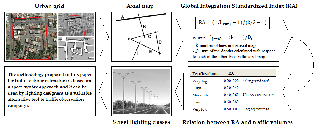
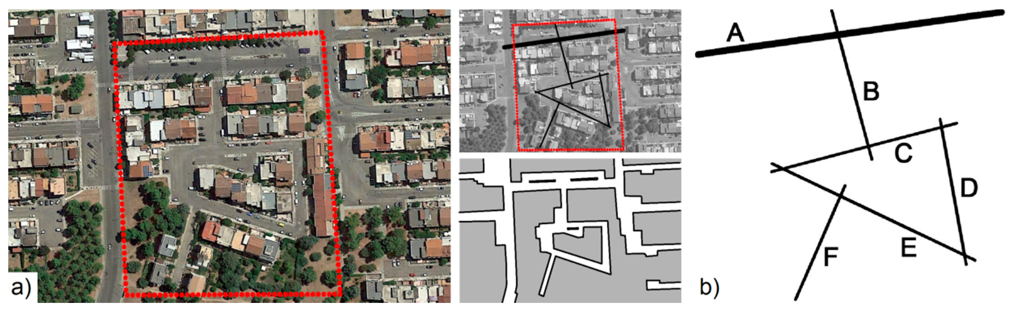
With the axial map, the space syntax analysis can be performed and syntactic measures can be produced. Syntactic measures give a numeric value to the graphic representation obtained with the axial map. Among the different syntactic measures, the global integration index (I_[r=n]) has been used. The global integration index measures the mean depth of an axial line [27]. The depth is measured as the topological (and not geometrical) distance separating two lines and is the number of lines that lie between the two lines considered. The number of lines is counted considering the shortest path between the two lines (see Figure 1). Global integration index is defined in Equation (1) as:

$${\mathrm{I}}_{\left[\mathrm{r}=\mathrm{n}\right]}=\left(\mathrm{k}-1\right)/{\mathrm{D}}_{\mathrm{t}}$$

(1)

where k is the number of lines in the axial map, and Dt can be obtained, for the considered line, as the sum of the depths calculated with respect to each of the other lines in the axial map. The global integration index gives a measure of how integrated or segregated a given line is from all the other lines of the axial map. Every road of a city is identified with one or more lines of the axial map, so the higher the integration index of a line in the axial map, then the busier and more integrated the road in the urban grid. On the contrary, the lower the value of the integration index of the road, the less busy the road.

The value of the mean depth of a line with respect all the other lines of the system (I_[r=n]) depends on the dimension k of the system. In fact, the value of the global integration index rises with the growth of the number of lines of the system: the larger the system, the greater the value of the global integration index. For this reason, the value of the global integration index is released from the dimension k of the urban grid with a procedure of standardization. The standardization procedure makes it possible to compare the I_[r=n] values of systems of different sizes. The standardization procedure is based on the concept of the relative asymmetry (RA), which relates to the comparison between the mean depth of a line and the minimum theoretically possible mean depth of the same line. The relative asymmetry is calculated as the ratio of two differences—the first difference at the numerator is between the mean depth of a line (1/I_[r=n]) and the minimum theoretically possible mean depth (always equal to 1), the second difference at the denominator is between the maximum theoretically possible mean depth and the minimum theoretically possible mean depth:

$$\mathrm{RA}=(1/{\mathrm{I}}_{\left[\mathrm{r}=\mathrm{n}\right]}-1)/\left(\mathrm{k}/2-1\right)$$

(2)

The RA is also called the “global integration standardized index” and ranges between 0 and 1. A value of RA = 0 is assumed in the case of a line directly connected to all the others. So, a line with RA = 0 is a line with a mean depth equal to 1 with respect to all the other lines. The value of RA = 1 is assumed in the case of a line at the end of a linear sequence of lines. The value of RA is always greater than zero and increases with the depth, that is, with the decrease of the integration. In fact, the minimum value is obtained for the most integrated line while the maximum value is obtained for the most segregated line. In conclusion, when the values of RA decrease, the traffic volumes increase; when the values of RA increase, the traffic volumes decrease.

2.2. Application Strategy to a Case Study

As already stated, this paper shows the application of a space syntax analysis for assessing traffic conditions as an alternative to traffic observation campaign. The strategy used can be summarized as follows: (a) space syntax analysis estimates traffic volumes in a urban grid, (b) an efficient public street lighting is adjusted to the actual traffic volumes in a urban grid, and (c) space syntax helps street lighting design to assess the traffic volume forecasted for a urban grid.

After performing the space syntax analysis of the analyzed urban center and calculating the value of RA for each road, traffic volumes were simply estimated as a function of RA compliant to the values (see

Table 1. Relationship between the global integration standardized index (RA) and the options of the traffic volume parameter prescribed by international standards (see Appendix 3), according to the adopted strategy.

Traffic Volumes	RA
Very high	0.00–0.20	+ integrated road
High	0.20–0.40
Moderate	0.40–0.60	Urban centrality
Low	0.60–0.80
Very low	0.80–1.00	− segregated road

). The range of RA values were divided into subranges in the same number of the possible options prescribed by current regulations for classify the traffic volumes. The best option of the traffic volume parameter was chosen depending on the value of the integration index (in Table 1, an example with the options of the traffic volume parameter prescribed by the CIE 115 technical report is shown).

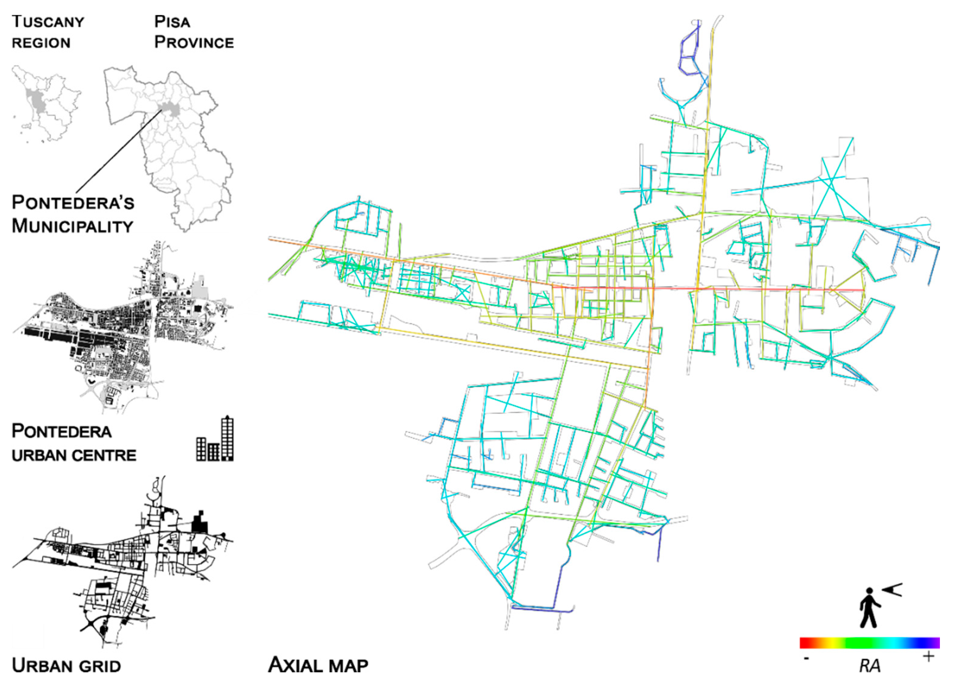
The town of Pontedera (Pisa, Italy) was chosen as the case study. Pontedera is a town of about 30,000 inhabitants, with a surface area of 46 km² and lies 30 km east of Pisa. Its urban center is located near the confluence of the Era River and the Arno River, and is bordered by the two rivers, the Scolmatore Canal, the Pisa–Florence railway and the motorway between Florence, Pisa, and Livorno.

3. Results and Discussion

Space syntax analysis, and in particular axial analysis, can be powered by specific software. In this paper, the UCL (University College London) Depthmap X software was used. The UCL Depthmap X software is released by the Centre for the Built Environment of the Bartlett School of Graduate Studies. The input data for the software was the urban grid of the town of Pontedera in a vector format (dxf file). The software produces outputs such as color charts and numeric tables that compare the various syntactic measures produced. Among the various syntactic measures, the global integration standardized index (RA) was used; the lower the RA value of a line in a system, the more accessible and integrated the line in the system.

The axial analysis of Pontedera town is represented in Figure 2 where the RA index is shown with a chromatic scale. The color scale runs from blue for the very highest values, to cyan, to green, to yellow, and up to red for the very lowest value [28]. The space syntax analysis used as a tool for assessing traffic volumes pedestrian and motorized in a town was studied. It was validated previously for many case studies [22,23,24,25,29,30,31,32,33]. Thus, it was assumed correct to validate the results obtained with the axial analysis for the town of Pontedera by carrying out a traffic observation campaign.

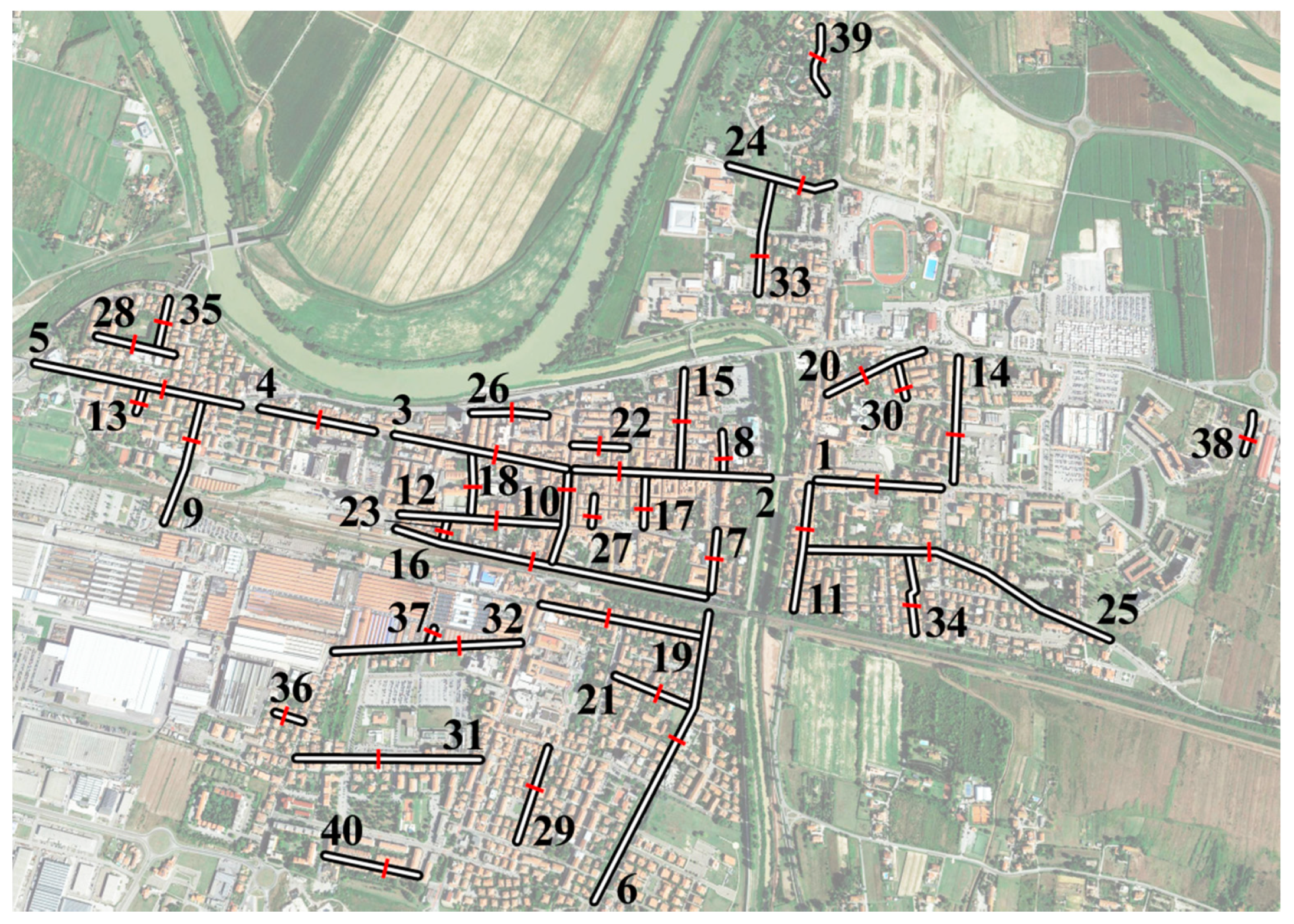
The pedestrian and motorized traffic observation campaign was performed on a sample of 40 roads, shown in Figure 3, corresponding to the 13% of all Pontedera roads (in Pontedera there are 305 roads). They were chosen to be representative of Pontedera roads. These roads were selected with the help of the axial analysis by using the following procedure. The values of RA were evaluated for all the roads of Pontedera (see Figure 2); calculating RA gave a minimum value (RA_min = 0.226) and maximum value (RA_max = 0.952). The roads were grouped into six categories (1. main roads, 2. roads of the historical center, 3. secondary roads, 4. roads connecting districts, 5. access roads to neighborhoods, and 6. neighborhood roads), each of them were obtained considering a constant increment of RA (from RA_min to RA_max with an interval of 0.121). Each group characterized by the RA range of values is shown in

Table 2. Grouping of Pontedera roads as a function of RA values.

Group	RA	Number of Roads		Road ID of the Restricted Sample
		Pontedera	Restricted Sample
1	0.226 ≤ RA ≤ 0.347	53 (17.4%)	7 (17.5%)	3, 5, 6, 8, 11, 12, 31
2	0.347 < RA ≤ 0.468	53 (17.4%)	7 (17.5%)	2, 14, 20, 22, 28, 39, 40
3	0.468 < RA ≤ 0.589	61 (20.0%)	8 (20.0%)	4, 15, 16, 17, 21, 23, 24, 25
4	0.589 < RA ≤ 0.710	92 (30.2%)	12 (30.0%)	7, 9, 10, 13, 18, 26, 27, 29, 30, 32, 34, 35
5	0.710 < RA ≤ 0.831	16 (5.2%)	2 (5.0%)	33, 37
6	0.831 < RA ≤ 0.952	30 (9.8%)	4 (10.0%)	1, 19, 36, 38
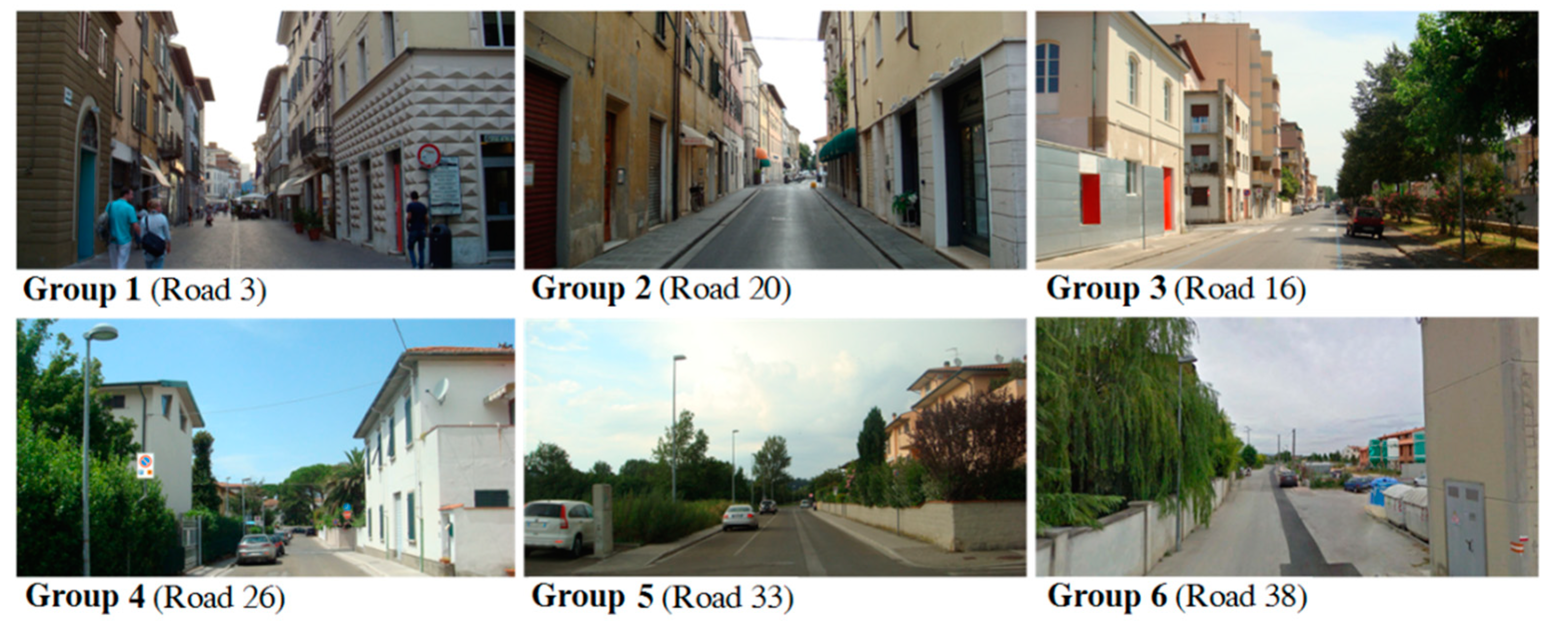
	Total	305 (100.0%)	40 (100.0%)

. For example, in the Pontedera historical center (group 2) there are 53 roads (17.4% of 305) and in the sample of the 40 roads that were selected, 7 roads were from group 2 (17.5% of 40). The sample of 40 roads was created by choosing a variable number of roads in each group, so as to reproduce the percentage distribution of the total roads in the six groups, as shown in Table 2. As an example, in Figure 4, the photographic images of six roads are shown, one for each of the six identified groups, with the relative RA values.

The pedestrian and motorized traffic observation campaign was conducted according to the so-called “gate method.” To conduct this observation campaign, a reference section for each individual road was selected (see Figure 3). The reference section has been selected so as not to be influenced by disturbing elements or specific points of possible aggregation of vehicles or pedestrians, such as crossroads, stops of public transport, entrances to important commercial or working activities, construction sites, traffic lights, etc. The parameters recorded during the observation campaign were: the number of vehicles and the number of passersby every 10 min. These parameters were recorded in the time slot from 17:30 to 19:30. The time slot was selected as the most intense (from the point of view of vehicular and pedestrian traffic) among all the time slots present in the period of ignition of the Pontedera street lighting system (which goes from sunset to sunrise). The observation campaign was carried out in the period October–November 2018. To guarantee the reliability of the observed data, a total of 3 observations were made for each road (on different days) and, for the subsequent processing, the average values of the recorded parameters were considered. The value of the traffic volume adopted in the correlation shown in the following graphs is the average value of the three measurements. The minimum value of the pedestrian traffic volume (averaged on three measures) was detected for road 38 with 3 passersby in 10 min while the maximum value was detected for road 2 with 183 passersby. The minimum value of motorized traffic volume (averaged on three measures) was detected for road 39 with 1 vehicle in 10 min while the maximum value detected was for road 2 with 178 vehicles. Correlation was carried out with a linear regression analysis performed using the least squares method and the coefficient of determination (R²) calculated. That is, the closer R² is to 1, the greater the goodness-of-fit for the linear model. The correlation was implemented between the RA and the measured traffic volumes.

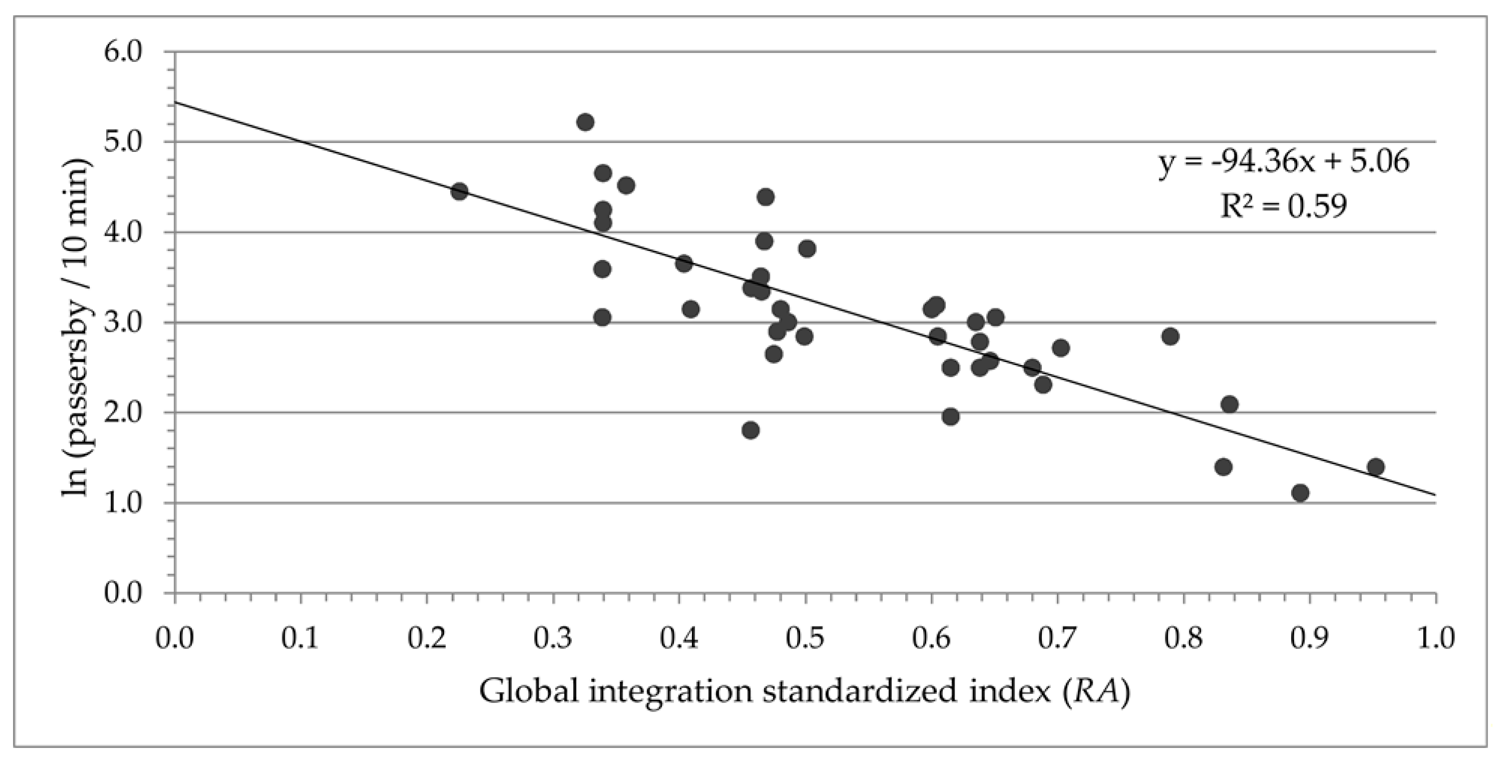
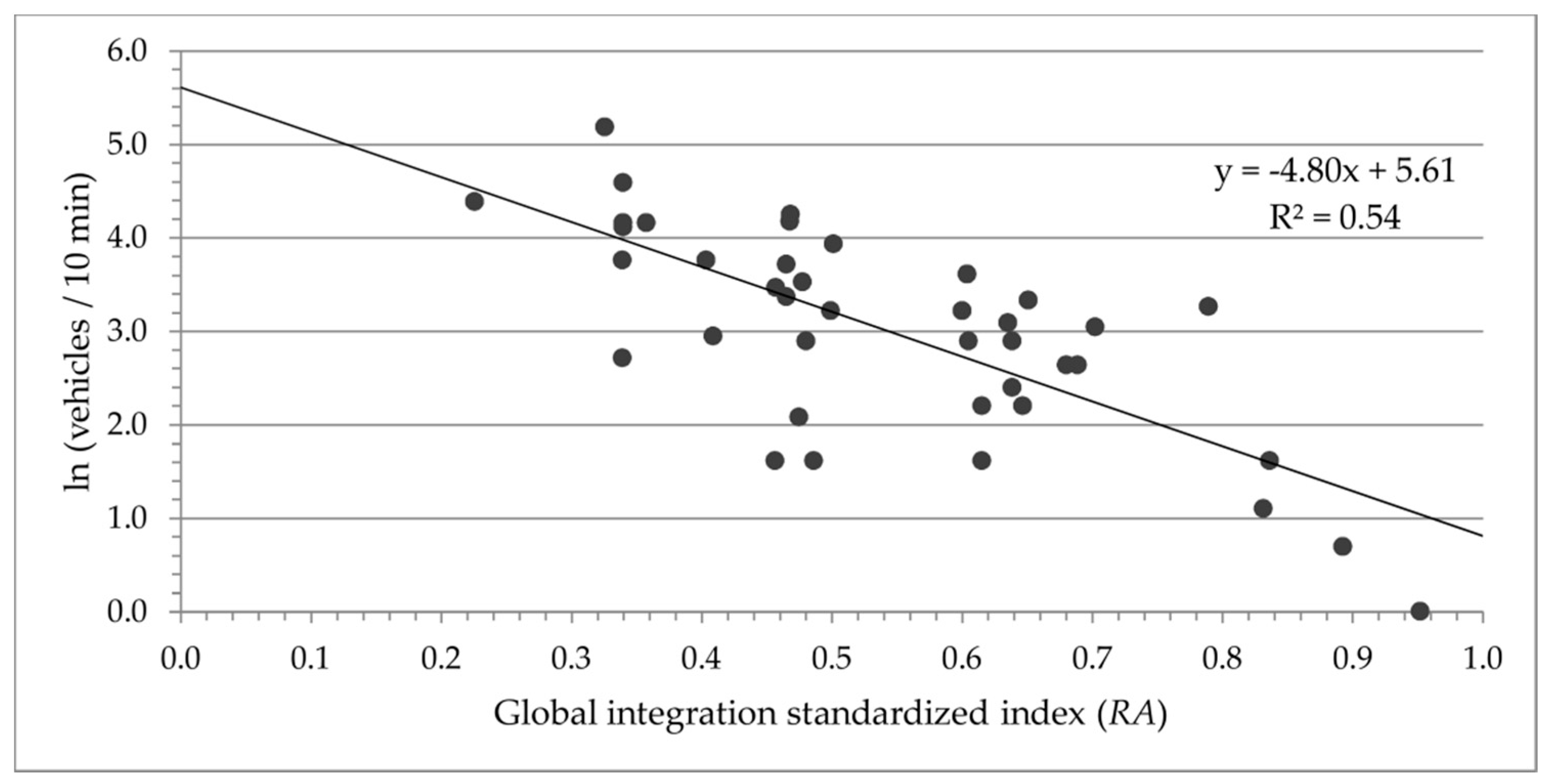
In Figure 5, the correlation between the logarithm values of the pedestrian traffic volumes measured for the 40 roads and the RA values of the same roads is shown (the pedestrian traffic volume value for each road is the average of three different measurements in three different days). The use of the natural logarithm was adopted on the basis of studies conducted on different English cities [34]. In Figure 6, the correlation between the logarithm values of the motorized traffic volumes measured in the 40 roads and the RA values of the same roads is shown (also in this case, the motorized traffic volume value for each road is the average of three different measurements in three different days). As can be observed, the correlation is robust enough. Nevertheless, the 40 roads of the restricted sample were subsequently grouped into 10 units of 4 roads with comparable RA values (each unit contains roads with a maximum RA deviation of 5%). For each unit, the mean value of the measured traffic volumes and the mean value of RA were calculated considering the road belonging to the unit. This procedure was implemented in order to reject data for values that were very different from the trend line, perhaps resulting from particular or temporary situations.

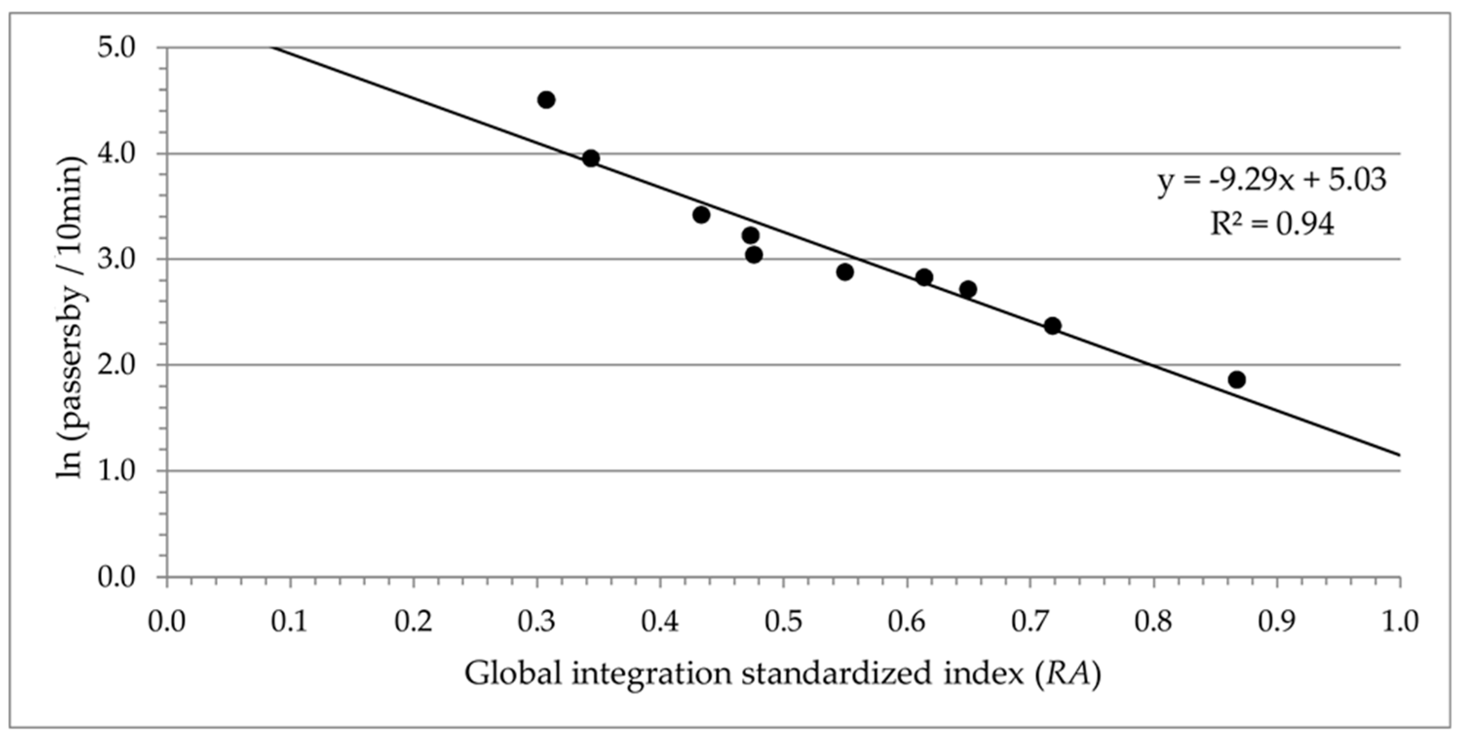
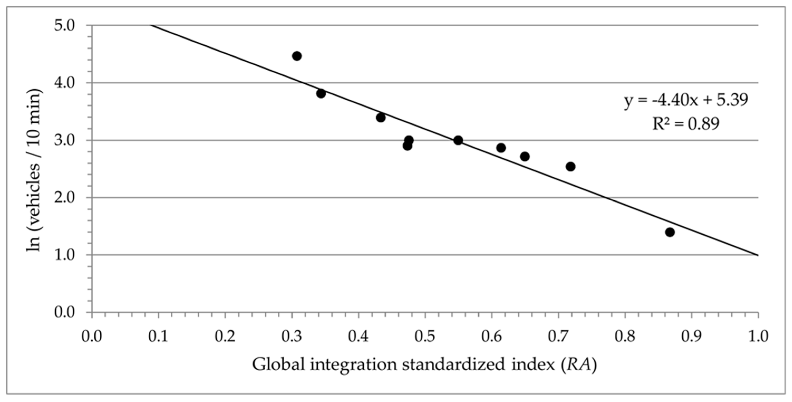
In Figure 7 and Figure 8, the correlation between the logarithm values of the mean traffic volumes, both for pedestrian and motorized traffic, obtained for each unit, and the related mean RA values are shown. The correlation shows a very significant coefficient of determination because its value is very close to the unit (R² = 0.94 for pedestrian traffic, R² = 0.89 for motorized traffic) confirming the validity of the axial analysis as a tool for forecasting traffic volumes in an urban center.

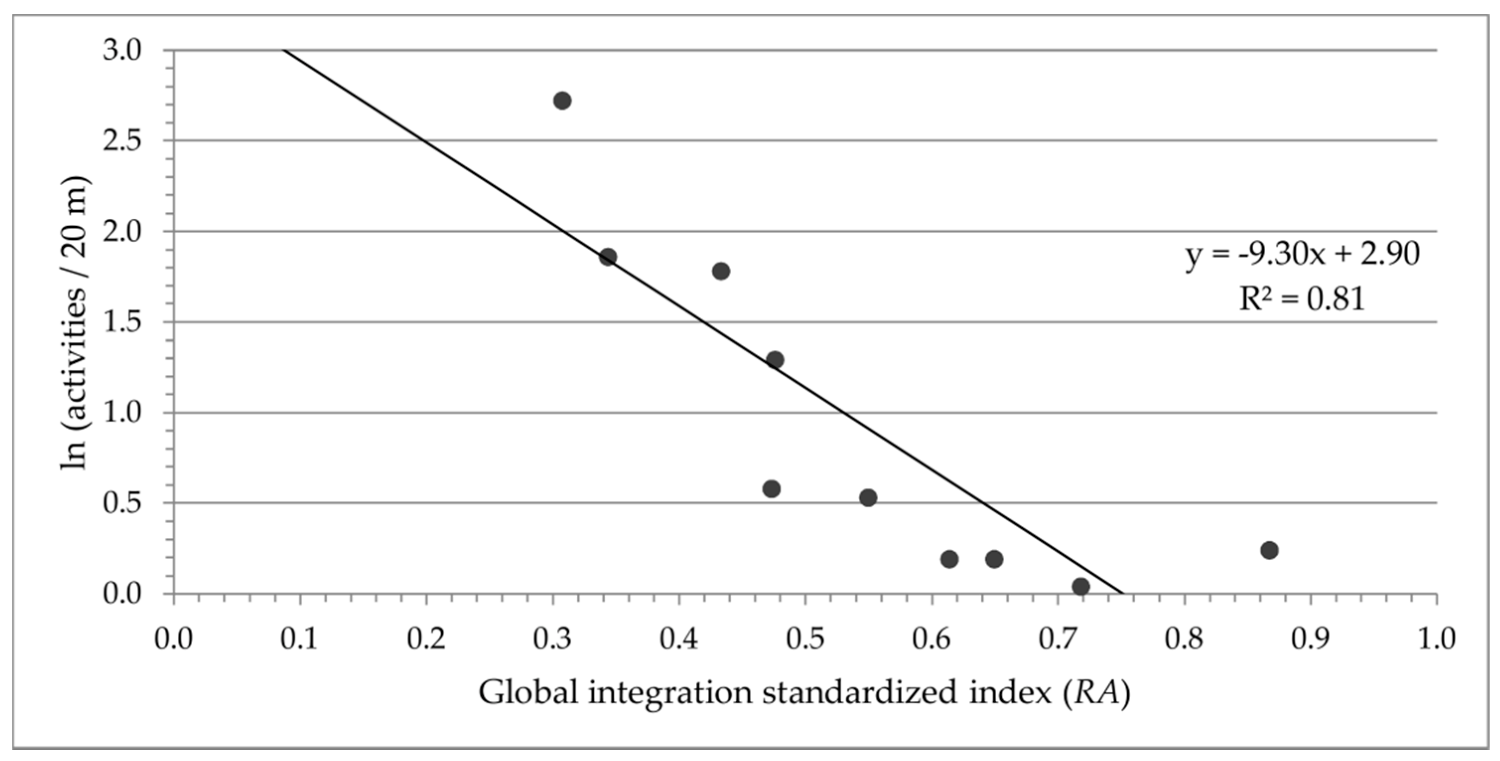
In Figure 9, the correlation between the logarithm values of the average number of activities (commercial activities, shops, other) every 20 m along roads, obtained for each unit, and the related RA values is shown. The high correlation (R² = 0.81) proves the initial hypothesis that the urban grid influences not only the pedestrian and motorized traffic volumes but also the positioning of human activities inside an urban center. As for traffic volumes, the average number of activities is correlated to RA through its natural logarithm.

In

Table 3. Results of street lighting classes determination.

Road ID	P*	P**	M*	M**
3	2	3	3	4
20	3	3	3	3
16	3	3	3	3
26	3	4	2	3
33	4	4	3	3
38	4	4	3	3

Legend. For each road: P* is the class for pedestrian areas, determined using the results of traffic observation campaign; P** is the class for pedestrian areas, determined using the results of space syntax analysis; M* is the class for motorized areas, determined using the results of traffic observation campaign; M** is the class for motorized areas, determined using the results of space syntax analysis.

, the results of street lighting classes determination are shown, as an application example, for the six roads represented in Figure 4 (one for each group indicated in Table 2). Table 3 shows the values of the lighting classes obtained according to the method described in the technical standard EN 13201-1 (see also the Supplementary Materials, Appendix 3). For both pedestrian areas (P) and motorized areas (M), the table shows the comparison between the classes obtained using the traffic flows recorded during the observation campaign (P*, M*) and those obtained using the estimated traffic flows through the RA values of each road according to Table 1 (P**, M**). As can be seen, the results are in good agreement, justifying a possible use of the described methodology as an alternative to the use of traffic observation campaigns.

The study on Pontedera town proves that integration values of the axial map provided a good forecast of the rates of movement along each road. The spatial integration affects the movement in two ways. First, a more integrated road has more probability than a segregated one to be chosen in paths between two roads. Second, a more integrated and central road is more easily reachable than a segregated and peripheral one since there are fewer roads interposed between the considered one and the others. That is, the more integrated roads will attract greater traffic volumes. The proportion of movement determined by these two ways, and thus attributable to the effects of the spatial layout itself, is called natural movement, as opposed to the additional movement called attracted movement due to the various activities (or attractors) located in the urban grid. Having a lighting design tool taking into account the actual traffic volume allows a more precise lighting classes selection with a greater calibration and a more precise design of the luminous fluxes, reducing as much as possible any energy waste and possible phenomena of light pollution.

Despite the encouraging results, the present study has some limitations, which arise from the simulations of the RA values by software and that are mainly linked to the estimation of vehicular traffic volumes in special situations and to the bidirectionality of traffic flows (both pedestrian and vehicular). For example, as evidenced also by other studies [35], with the software used it is not currently possible to separately consider a vehicular traffic-restricted area, often present in a grid of urban roads, and it is not possible to evaluate the traffic volumes as a function of their directions, because the distinction of unidirectional and bidirectional roads is not allowed. Another problem is the edge-effect because the analysis is unable to consider the traffic towards and away from the city [36,37]. Improving the accuracy of this kind of simulation represents a challenge for the scientific community, just as it is desirable that other research groups test the procedure described in this study for other cities worldwide.

4. Conclusive Remarks

Public street lighting is an element of very considerable importance in the urban night panorama as it contributes to traffic management, visual comfort, and user perception of security. On the other hand, public lighting service demands a large share of the economic budget of public administrations. This is true, not only for road surfaces, but also for sidewalks, paths, and pedestrian areas. For this reason, illuminance levels on each connected area must be weighted on the basis of the actual traffic volumes to avoid energy waste and oversized lighting systems. Traffic volume is the most incisive parameter for the calculation of the minimum safety requirements prescribed by current regulations. At the same time, traffic volume is the most expensive parameter to evaluate because it is time consuming if a classic traffic observation campaign is adopted. The methodology described in this paper for traffic volume estimation can be used by lighting designers as a valuable alternative tool to a traffic observation campaign because space syntax analysis proved to be easier and faster than classical methods. Most important, space syntax analysis revealed a powerful tool in forecasting pedestrian and motorized traffic volume as demonstrated for the city of Pontedera and from the extensive research reported in scientific literature. With a better knowledge of traffic conditions, a greater calibration of the installed power is possible to achieve reduced energy waste and, therefore, improve the energy sustainability of the lighting systems. The method can be extended to motorized traffic analysis, although some issues must be overcome. Economic savings that could be obtained from the reduction in energy consumption should not be neglected. Economic savings would make available a share of public resources with the possibility to reallocate public money savings to other activities. Finally, the method is particularly useful in the planning of lighting systems of new roads or areas yet to be developed, for which it would obviously be impossible to carry out a traffic observation campaign and so traffic volumes could only be estimated.