Optimal Energy Management in a Standalone Microgrid, with Photovoltaic Generation, Short-Term Storage, and Hydrogen Production

Abstract

This paper addresses the energy management of a standalone renewable energy system. The system is configured as a microgrid, including photovoltaic generation, a lead-acid battery as a short term energy storage system, hydrogen production, and several loads. In this microgrid, an energy management strategy has been incorporated that pursues several objectives. On the one hand, it aims to minimize the amount of energy cycled in the battery, in order to reduce the associated losses and battery size. On the other hand, it seeks to take advantage of the long-term surplus energy, producing hydrogen and extracting it from the system, to be used in a fuel cell hybrid electric vehicle. A crucial factor in this approach is to accommodate the energy consumption to the energy demand and to achieve this, a model predictive control (MPC) scheme is proposed. In this context, proper models for solar estimation, hydrogen production, and battery energy storage will be presented. Moreover, the controller is capable of advancing or delaying the deferrable loads from its prescheduled time. As a result, a stable and efficient supply with a relatively small battery is obtained. Finally, the proposed control scheme has been validated on a real case scenario.

1. Introduction

One of the most important elements in the modern is energy, which has usually been obtained from fossil fuels. However, their availability is limited, and their negative effects on the environment have been widely reported. A lot of research has been performed on the social-economic impact of CO${}_2$ emissions [1], and the possible collapse of a society with finite energy sources [2]. In consequence, the interest in developing renewable energy sources (RES) and increasing its energy market share has rapidly grown in recent years. As a result, the transition to renewable energy poses new challenges, due to its intrinsic characteristics.

On the one hand, power systems require a continuous balance between the demand and supply of energy. Nevertheless, the variability and unpredictability of renewable sources, particularly wind and solar, may cause deviations in the parameters of the supply network [3]. An approach to renewable integration is to compensate the variability with short-term energy storage subsystems (ESS) [4], which can store the surplus energy and supply it when the generation is insufficient. On the other hand, the ubiquity of the solar resource allows the generation to be distributed near the points of use. Thus, the integration of renewable energy has encouraged the decentralization of power systems, through distributed generation and storage. In the literature, on-site generation and ESS are usually called “distributed energy resources” (DERs) [5]. The implementation of DERs and consumption points that can be disconnected from the utility grid, working autonomously and acting as a single controllable entity is usually named a microgrid [5].

Regarding standalone systems, there are several available options in terms of components, system architecture, and configuration [6]. The energy production depends on renewable resources, which presents variability and uncertainty. In consequence, the design and sizing of the system based in solar energy is a complex task [7], which requires estimating the balance between production and consumption [8]. As for the photovoltaic generation, in addition to its size other characteristics must be determined, such as the orientation and tilt of the solar panels. All this will determine energy production, but always depends on the variations of the solar resource. In the short term, ESS can follow the demand curve, if there is enough stored energy. In fact, to obtain some security for the energy supply, it is necessary to oversize the photovoltaic system, the ESS, or both. As a result, there will be a surplus of energy in the long term. In practice, the oversize can be avoided by hybridization with diesel generation [9]. This is one of the main causes that make it difficult to achieve the economic optimum of a standalone system with 100% RES. Therefore, it is important to reduce the need for oversizing and, if possible, to harness the energy surplus.

One of the key parts of the technical and financial viability of the microgrid is the selection of an adequate storage system. The lead-acid battery is a relatively economic ESS, widely used in microgrid applications however, lead-acid batteries present a short lifetime, especially in cycling operations [10]. In order to minimize the economic costs and degradation of the storage system, the optimal battery size has to be determined [11]. For this reason, several technical and financial indicators must be considered, including an estimation of the effort of the battery throughout its lifetime.

From a manageability point of view, energy sources can be classified as dispatchable sources (for example, a genset) or non-dispatchable sources (for example, wind turbines or photovoltaic arrays). Similarly, loads accept a similar classification, non-deferrable loads (whose operating timing cannot be modified), and deferrable ones (whose operating timing can be managed in a flexible manner) [12], the so-called demand side management (DSM) [4]. Thus, dispatchable sources and deferrable loads offer additional degrees of freedom to improve system performance if they are properly handled. Efficient control schemes may reduce the effort of the battery, therefore reducing operational costs of the energy storage system and, proportionally, of the microgrid system. The model predictive control (MPC) is a suitable control scheme for this type of system. Multiple works can be found in the literature that describe the benefits of this control strategy. There are examples of MPC algorithms being applied to minimize operating costs of energy storage systems [13], optimize a multiobjective cost function in AC/DC microgrids [14], control an offshore wind farm [15], control a reconfigurable inverter in a standalone PV-wind-battery microgrid [16] and control a microgrid with hydrogen production and consumption [17].

In this paper, the MPC technique is used in the context of a standalone microgrid, which supplies the energy demanded for the wastewater treatment plant of a winery. The generation of this microgrid is 100% photovoltaic. That is, in the microgrid under study, some loads are deferrable while the energy sources are non-dispatchable. The main contribution of this work is to propose an energy management strategy that will optimally manage the design performance taking into account the loads and RES characteristics. The proposed methodology will be based on the MPC. This type of algorithm requires forecasting the RES and loads behavior. As the microgrid will operate in island mode, isolated from the main grid, a methodology to predict the RES behavior will also be included in the algorithm. The main novelty of this work is the combination of a relatively simple and comprehensive model, which includes: A solar irradiance prediction algorithm, a battery model, and a hydrogen generation model with a MPC algorithm that, through re-scheduling of deferrable loads and controlling the solar panel’s power output, reduces the microgrid’s battery cycling. The proposed control scheme is shown to be implementable in a real case scenario and is compared with an existing energy management system. It is shown that the presented scheme provides a better matching between the demand and supply, improves the microgrid’s reliability, and reduces battery effort.

The work is organized as follows, Section 2.1 contains a description of the different elements which compose the microgrid; Section 2.2 describes the methodology used to predict the solar irradiance; Section 2.3 describes the battery model and its tuning; Section 2.4 contains a description of the hydrogen facility; and Section 3.3 describes the control problem and the developed energy management algorithm. Section 4 contains several results and finally Section 5 contains some conclusions, limitations, and future works.

2. System Modeling

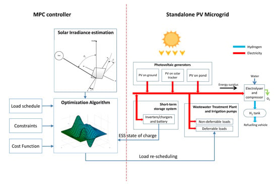
This section describes the microgrid that will be considered. It corresponds to the standalone RES placed at the Viñas del Vero winery, which is located in the Somontano region, in the north of Aragon (Spain) [18,19]. The energy consumed in the winery’s wastewater treatment plant and the irrigation system is supplied with a set of photovoltaic panels. Furthermore, a lead-acid battery is used as a short-term ESS and the surplus energy produced by the PV system is converted into hydrogen by water electrolysis. This hydrogen is eventually supplied to a fuel cell hybrid electric vehicle. In Figure 1, a general scheme of the system is depicted. All variables and parameters used in the model are depicted in

Table 1. Description of the model variables and parameters.

Variable Name	Description	Variable Name	Description
$G_{sc}$	Solar constant	n	number of the day
$G_{on}$	Corrected solar constant	${\eta }_p$	Solar panel’s efficiency
$\varphi$	Latitude	${\eta }_{inv}$	Inverter’s efficiency
$\delta$	Declination	$P_{out}$	Potential panel’s power output
$\beta$	Slope	$P_{SOL}$	Solar panel’s power output
$\gamma$	Surface azimuth angle	$SOC$	State of Charge
$\omega$	Hour angle	$I_{BAT}$	Battery’s current
${\theta }_z$	Zenith angle	$U_{BAT}$	Battery’s open circuit voltage
$\theta$	Angle of incidence	$R_{BAT}$	Battery’s internal resistance
$G_{b,\tau }$	Extraterrestrial irradiance	$U_{BAT}$	Battery’s terminal voltage
$T_L$	Turbidity coefficient	$P_c$	Power consumption
$I_{cs}$	Clear-sky DNI	$C_{rate}$	C rate
b	Correction coefficient	$DOD$	Depth of Discharge
m	Relative optical air mass	$Ah$	Effective Ah-throughput
h	Solar panel’s height	$\sigma$	Severity factor
I	Measured normal irradiance	$Bl$	Battery charge/discharge efficiency
N	Number of solar panels	$A{h}_n$	Nominal Ah-throughput
$P_{BAT}$	Battery’s power	$C_n$	Nominal capacity
$I_{BAT}$	Battery’s current	${\alpha }_{ch/dch}$	Battery’s charge/discharge efficiency

.

2.1. Description of the Facilities

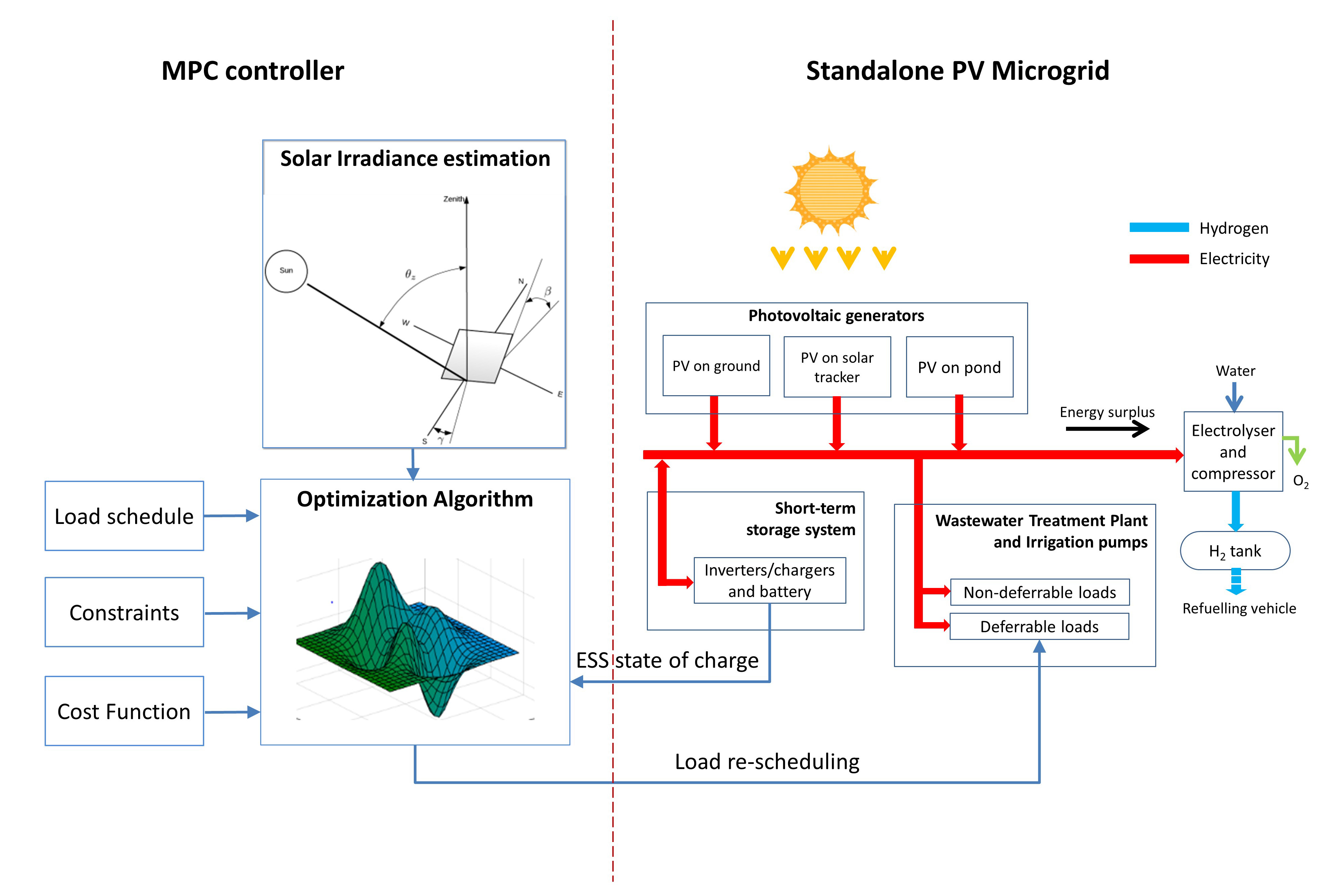
The microgrid electrical distribution network was designed with an AC bus architecture, to which the PV panels, the battery, and the power consumers are directly or indirectly connected. It operates at 400 V and 50 Hz, and it is regulated by the inverters connected to the battery. No connection to the general distribution network exists, i.e., the microgrid works in isolated operation mode.

The system could work without the production of hydrogen. However, as usual in standalone systems with 100% renewable generation, there would be a high percentage of surplus energy, which could not be used. This happens when the production is greater than the consumption and the battery is fully charged. This hydrogen is extracted from the system, by refuelling a fuel cell electric vehicle.

2.1.1. Solar Photovoltaic System

A set of solar photovoltaic panels is used as the main energy source. Three different PV arrays on different supports are available: A fixed structure on the ground, a floating structure on the pond of the wastewater treatment plant, and a two-axis solar tracker.

The DC power generated by the solar panels is transferred to the AC bus through a group of DC/AC three-phase solar power inverters. These inverters include maximum power point trackers (MPPT) to ensure that the solar cells work at the optimum point of their voltage-current curve, which varies depending on the incident radiation. The inverters can be regulated to produce only a percentage of the available energy. Thus, in terms of the energy management algorithm the solar inverters will be a controllable input of the system.

2.1.2. The Battery Storage System

The microgrid contains a lead-acid battery bank which is used as a low-term ESS. The battery is connected to the AC bus through a set of battery inverters (one for each phase). These inverters are also responsible for maintaining the voltage and frequency parameters of the microgrid.

2.1.3. The Power Consumers

The PV electric power is used to supply the winery’s wastewater treatment plant and the irrigation system. Specifically, this energy demand includes the power consumed by the water treatment plant (aerators), a set of elevation pumps used for irrigation, and a system of hydrogen production used to fuel a hybrid electrical vehicle [20]. Moreover, the aerators are power loads that can be advanced or postponed from its scheduled time. This re-schedule of the load will be managed by the controller proposed in this work.

2.2. Estimation of Solar Irradiance

The energy production system is a set of solar panels, which transforms solar radiation into electric energy. In order to design a predictive control, it is necessary to have some knowledge about the future of the system. Although nowadays there exist excellent weather forecast services they are usually available in isolated areas. Thus, it is crucial to develop a model that forecasts the solar resource received by the panels, and more specifically, its clear-sky direct normal irradiance (DNI).

In the literature, clear-sky DNI is defined as the direct solar irradiance that did not interact with the atmosphere and is received by a plane normal to the sun [21]. Two types of clear-sky DNI forecasting models can be found in the literature: Radiative transfer models and empirical ones [22]. Radiative transfer models are based on an accurate estimation of the atmosphere’s state. Although this type of model estimates clear-sky DNI with really high accuracy [23], it is necessary to compute complex calculations using data difficult to be obtained. As a consequence, radiative transfer models are not convenient for predictive control. In this work, an empirical model based on [24] is used.

2.2.1. Solar Constant

The solar constant $G_{sc}$ is the solar radiation per unit of time received on a unit area of a surface perpendicular to the direction of circulation of the radiation at an average earth-sun distance without considering the atmosphere [25]. A constant value of $G_{sc}=1360.8$ W/m${}^2$ [25] is the most used value in the industry however there are some sources of variation. The elliptic orbit of the earth around the sun induces a variation, up to 3.3%, of the solar radiation. This dependence can be represented by the following equation [26]:

$$G_{on}=G_{sc}\left(1+0.034cos\left({\displaystyle \frac{2\pi n}{n_d}}\right)\right)$$

(1)

where $n_d$ is the number of days in the year, $n_d$ = 365 or 366 (leap-years). And n is the day number, $n\in [1,n_d]$. The modified solar constant ($G_{on}$) represents the power received from the sun on a plane normal to the direction of propagation.

2.2.2. Geometric Considerations

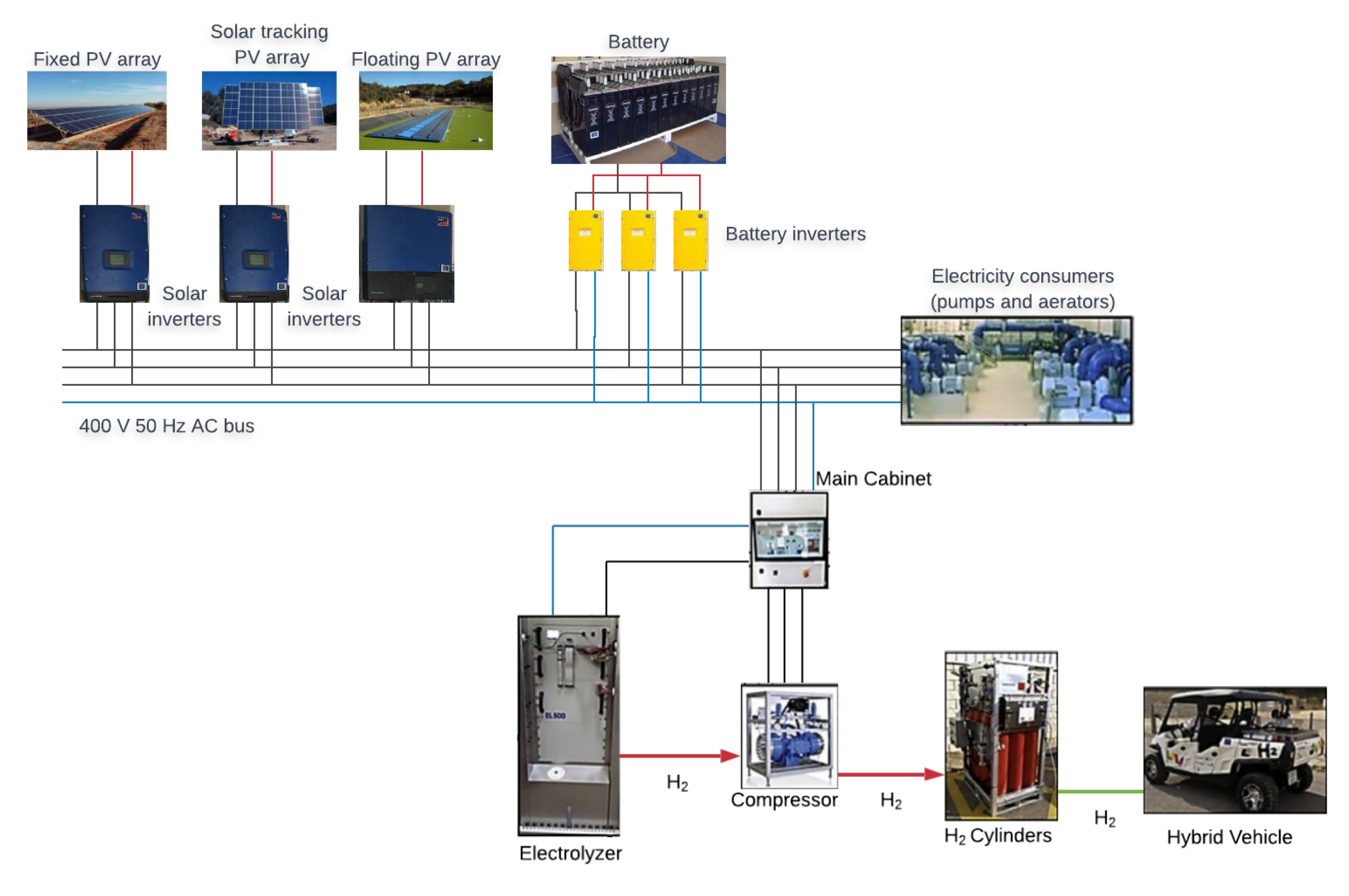
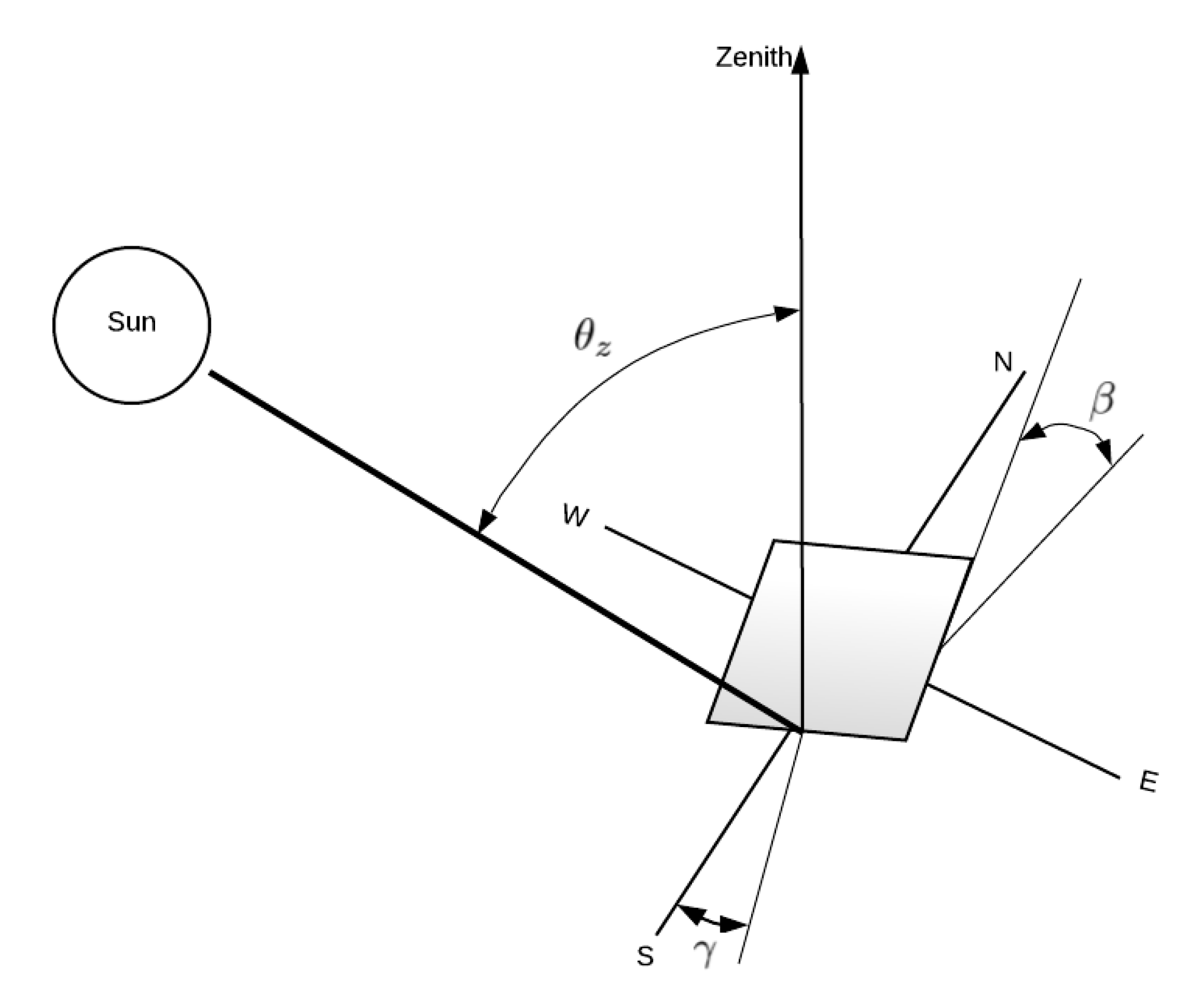
Solar panels may not always be normal to solar radiation, thus it is necessary to define the geometric relationship between the solar radiation and a surface arbitrary oriented and positioned on earth. With this objective in mind, a set of angles is defined as depicted in Figure 2:

• Latitude ($\phi$): Geographic coordinate that specifies the north-south position of the surface’s center;

  $$-90°\le \phi \le 90°$$
• Declination ($\delta$): The angular position between the sun on the local meridian and the plane of the equator;

  $$-23.45°\le \delta \le 23.45°$$
  Which can be estimated with the following equation [27]:

  $$\delta =23.45sin\left(2\pi {\displaystyle \frac{284+n}{n_d}}\right)$$

  (2)

  where $n_d$ and n are defined in Equation (1);
• Slope ($\beta$): The angle between the surface’s plane and the horizontal plane;
• Surface azimuth angle ($\gamma$): Angle between the surface’s vector of the perpendicular projection on a horizontal plane and the south vector;

  $$-180°\le \gamma \le 180°$$
• Hour angle ($\omega$): The angular variation of the local meridian due to rotation of the earth, at 15 per hour;

  $$-180°\le \omega \le 180°$$
• Zenith angle (${\theta }_z$): Angle between the solar radiation and the zenith of the panel;

  $$-90°\le {\theta }_z\le 90°$$
• Angle of incidence ($\theta$): Angle between the direct radiation on a surface and the normal to that surface;

The angle of incidence can be derived from this set of angles [28] as follows:

$$\cos \theta =\sin \delta \sin \phi \cos \beta -\sin \delta \cos \phi \sin \beta \cos \gamma +\cos \delta \cos \phi \cos \beta \cos \omega +\cos \delta \sin \phi \sin \beta \cos \gamma \cos \omega +\cos \delta \sin \beta \sin \gamma \sin \omega$$

(3)

The angle $\theta$ may exceed the 90°, which means the sun is behind the surface. In photovoltaic applications this fact implies null generation from the panels.

2.2.3. Geometric Considerations for Tracking Surfaces

The solar photovoltaic system includes a PV array mounted on a two-axis solar tracker, which continuously changes the surface slope ($\beta$) and azimuth angle ($\gamma$) in order to minimize the angle of incidence and to maximize the solar irradiance captured by the panels. In this context, the following assumption can be made $cos\theta =1$.

2.2.4. Extraterrestrial Irradiance

The defined set of angles and the modified solar constant can be used to estimate the solar radiation received by the panels as $G_{b,\tau }=G_{on}cos\theta$. This estimation does not include the effects of the atmosphere and, for this reason, the calculated irradiance is known as extraterrestrial irradiance.

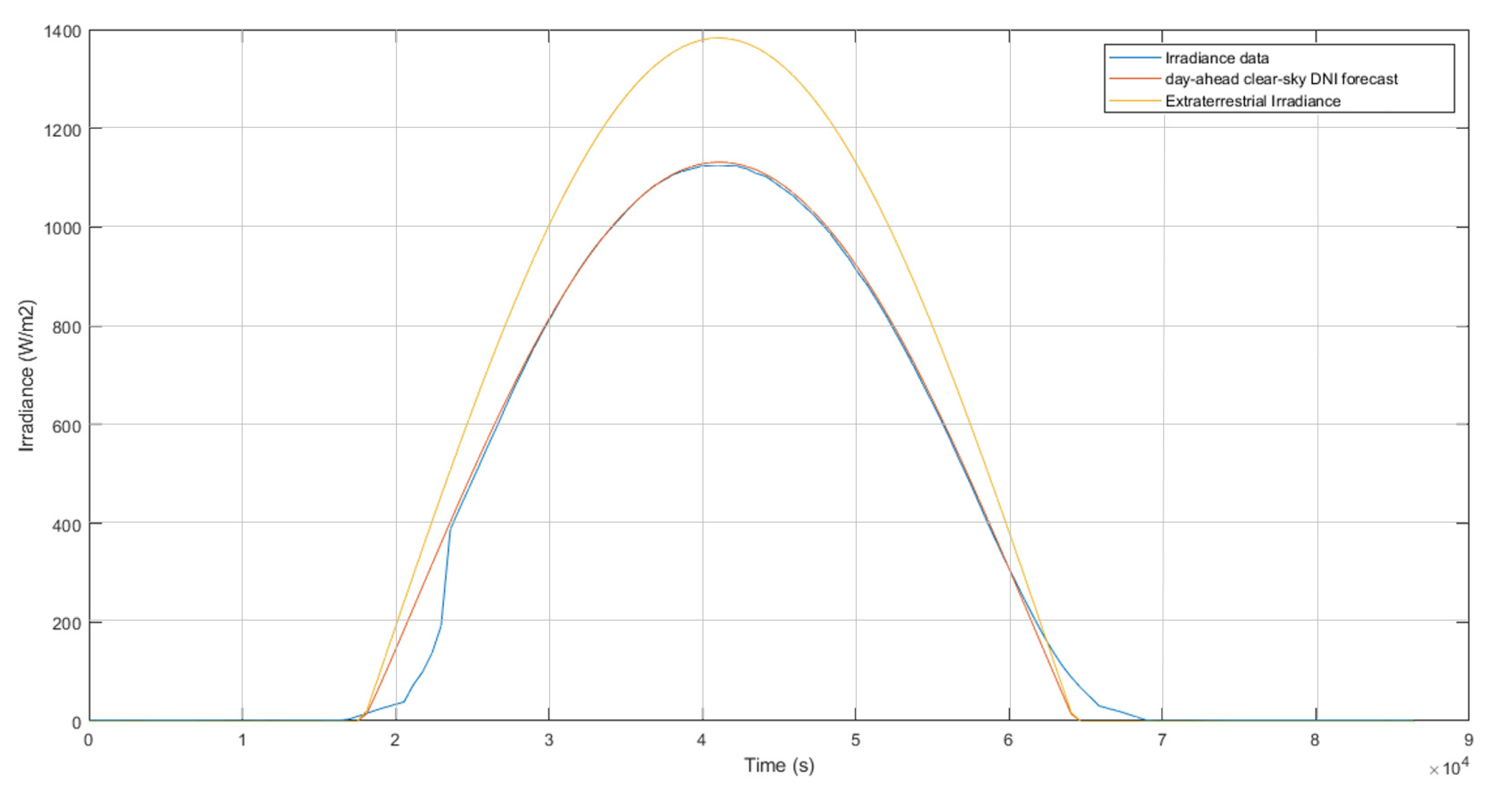
Each PV array include a pyranometer that measures the solar irradiance that reaches perpendicularly the panels’ plane. In Figure 3, the difference between the computed extraterrestrial radiation and actual irradiance measured at the panels’ pyranometer is shown.

It can be seen that the extraterrestrial irradiance values are significantly higher than the measured ones. This is due to the fact that the solar radiation must cross the earth’s atmosphere and react with its elements before reaching the solar panels. The inclusion of this attenuation in the model is explained in Section 2.2.5.

2.2.5. Atmospheric Attenuation and Clear-Sky Irradiance

Solar radiation is subject to variations as it crosses the terrestrial’s atmosphere. Under cloudless skies, there are two significant phenomena that induce some attenuation to the solar radiation:

• Scattering as the radiation interacts with the atmospheric molecules;
• Absorption of the radiation by the molecules $O_3$, $H_{2}O$, and $C{O}_2$.

In [24] a model of the atmosphere attenuation based on a modification of the Kasten-reviewed Linke turbidity coefficient ($T_L$) [29] is proposed as:

$$I_{cs}=b{G}_{b,\tau }{e}^{-0.09m\left(T_L-1\right)},$$

(4)

where $I_{cs}$ is the attenuated extraterrestrial irradiance or clear-sky DNI and b is a correction coefficient defined as follows [24]:

$$b=0.0664+0.163e^{\left({\displaystyle \frac{h}{8000}}\right)}.$$

(5)

The parameter h is the panel’s height above sea level in meters and m is the relative optical air mass. In [30] a formulation dependent on the zenith angle (${\theta }_z$) is proposed:

$$m={\displaystyle \frac{1}{cos{\theta }_z+0.1013{\theta }_z{\left(94.37515-{\theta }_z{\displaystyle \frac{180}{\pi }}\right)}^{-1.21563}}}.$$

(6)

The value $T_L$ is the modified Linke turbidity coefficient and can be computed in the following way [24]:

$$T_L={\displaystyle \frac{11.1}{m}}ln\left({\displaystyle \frac{b{G}_{b,\tau }}{I}}\right),$$

(7)

where I is the normal irradiance measured by a pyranometer located at the surface of the solar panel.

As illustrated in [21] the turbidity coefficient is relatively stable throughout cloudless daylight hours. In [31] the following day-ahead clear-sky DNI forecast is proposed:

$$I_{cs}=b{G}_{b,\tau }{e}^{-0.09m\left(T_{L,n-1}-1\right)},$$

(8)

where $T_{L,n-1}$ is the daily mean value of the atmospheric turbidity of the previous day and n is the number of the day $n\in [1,n_d]$.

Moreover, in the computation of $T_{L,n-1}$, two constraints are imposed:

• Atmospheric turbidity values corresponding to solar zenith angles greater than 75° are removed;
• A minimum number of 60 clear-sky data is needed. Otherwise, the most recent historical clear-sky data is used.

In Figure 3, the difference between the actual irradiance measured at the panels’ pyranometer, the computation of the day-ahead clear-sky DNI forecast, and the computed extraterrestrial irradiance is represented. It can be seen that the model presented in this section forecasts the clear-sky DNI with more precision than the extraterrestrial irradiance model. Using the root mean square error (RMSE) as a performance indicator, it can be observed that the RMSE has been reduced from 142.36 ${\displaystyle \frac{W}{m^2}}$ to 35.13 ${\displaystyle \frac{W}{m^2}}$.

2.2.6. Solar Energy Conversion

The solar panels convert solar radiation into DC electric energy, which will be converted into an AC current through the corresponding power inverters. In this process, a series of efficiencies must be taken into account.

• Solar panel efficiency$\left({\eta }_p\right)$: Relation between the solar radiation perpendicular to the panel surface and the output of electric energy from the panel;
• Inverter efficiency$\left({\eta }_{inv}\right)$: Relation between the output AC electric energy and the input of DC electric energy.

Thus, the electric energy that the AC bus will receive from the solar panels can be estimated for any given solar radiation by:

$$P_{output}=NS{\eta }_{inv}{\eta }_p{I}_{cs}$$

(9)

where N is the number of solar panels, S is its individual area, and $I_{cs}$ is the perpendicular solar radiation that reaches its surface.

In this work, a set of solar inverters acts as an interface between the DC grid of the solar panels and the AC bus of the microgrid. These inverters can be controlled for power regulation between the photovoltaic system and the microgrid. Therefore, the electrical energy introduced to the system through the solar panels’ inverters ($P_{SOL}$) is a controllable input of the microgrid. Obviously, this input will be bounded by the available solar energy, i.e., $0\le P_{SOL}\le P_{output}$.

2.3. The Battery Storage Model

2.3.1. Battery Model

A battery is an electrochemical device capable of converting chemical energy into an electrical one (discharging) and vice versa (charging). In order to implement a predictive management strategy, a model that approximates the battery’s performance is needed.

In energy management systems, an essential variable is the amount of energy stored in the battery, which can be quantified with the state of charge (SOC). The definition of SOC is the ratio of the remaining capacity to the nominal capacity of the battery, which can be described as,

$$SOC={\displaystyle \frac{1}{C_n}}{\int }_0^{t_f}{I}_{BAT}dt.$$

(10)

Thus, the prognostication of the battery’s SOC consists in an estimation of the future charging and discharging currents ($I_{BAT}$), which can be deduced from the prediction of the energy generated by the photovoltaic panels and the scheduled energy consumption of the system. Assuming that the MPC will work with a low sampling rate, a quasi-stationary model of $I_{BAT}$ evolution could be implemented.

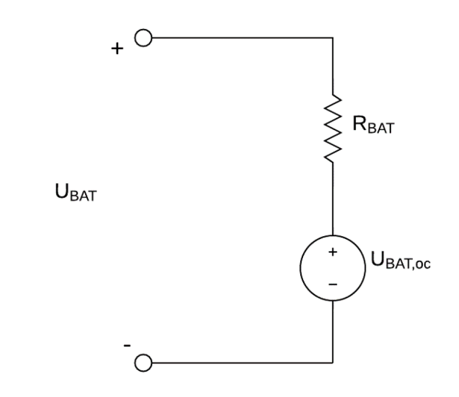
The battery can be modeled as a voltage source ($U_{BAT,oc}$), also called open circuit voltage, connected to an internal resistance ($R_{BAT}$) [32]. The circuit is depicted in Figure 4. In this scheme, the terminal voltage of the battery is given by:

$$U_{BAT}=U_{BAT,oc}-R_{BAT}{I}_{BAT},$$

(11)

where $U_{BAT}$ is the terminal voltage. The current yielded by the battery is computed from the power demanded to the battery $P_{BAT}$:

$$\begin{array}{ccc}\hfill P_{BAT}& =& U_{BAT,oc}{I}_{BAT}-R_{BAT}{I}_{BAT}^2\hfill \end{array}$$

(12)

$$\begin{array}{ccc}\hfill I_{BAT}& =& {\displaystyle \frac{U_{BAT}-\sqrt{U_{BAT,oc}^2-4R_{BAT}{P}_{BAT}}}{2R_{BAT}}}\hfill \end{array}$$

(13)

where $I_{BAT}$ is defined positive while discharging.

Furthermore, the battery’s open circuit voltage ($U_{BAT,oc}$) depends on the state of charge (SOC) and several other factors as thermal effects and filtered battery current [33]. In the microgrid under consideration the batteries are inside a temperature-controlled room, so temperature can be assumed constant and thermal effects will not be taken into account.

Described battery equations are nonlinear, this makes it difficult to apply optimizers, so a linear version of them has been developed. With this perspective, the battery charging/discharging current ($I_{BAT}$) can be assumed to be constant and equal to the nominal value $I_{BAT}=I_{BAT,nom}$. Consequently the open circuit voltage can be considered nearly constant [34].

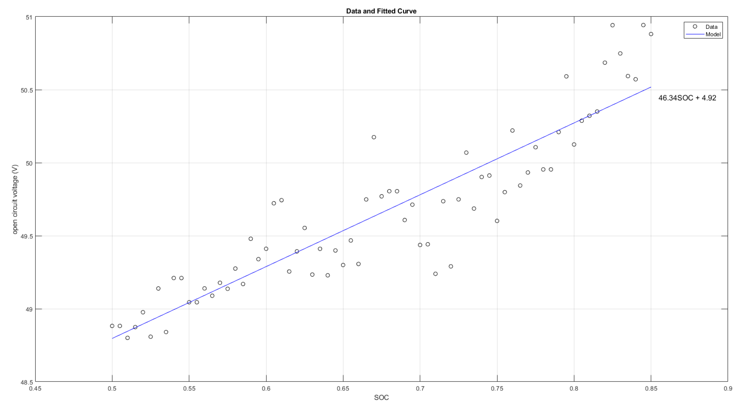
Figure 5 shows the battery open circuit voltage, obtained from experiments, as a function of the SOC. In the range $0.5\le SOC\le 0.85$ the variation of $U_{BAT,oc}$ is less than 2 volts, it allows one to validate the previous assumption.

Battery losses can be characterized through constant efficiencies ${\alpha }_{ch}/{\alpha }_{dch}$. Consequently, the following linear characterization of the battery SOC can be developed from Equation (10):

$${\displaystyle \frac{dSOC}{dt}}={\displaystyle \frac{1}{C_n}}{I}_{BAT}={\displaystyle \frac{1}{C_n{U}_{BAT,oc}}}{P}_{BAT}$$

(14)

The power that is charged or discharged from the battery $P_{BAT}$ depends on the difference between the power generated by the photovoltaic panels, $P_{SOL}$, and the power consumed by the system $P_c$. Hence, two expressions can be obtained from Equation (14):

$${\displaystyle \frac{dSOC}{dt}}=\left\{\begin{array}{cc}{P}_c\le P_{SOL}\hfill & {\displaystyle \frac{1}{C_n{U}_{BAT,oc}}}{\eta }_{inv}{\alpha }_{ch}\left(P_{SOL}-P_c\right)\hfill \\ P_c>P_{SOL}\hfill & {\displaystyle \frac{1}{C_n{U}_{BAT,oc}}}{\eta }_{inv}{\alpha }_{dch}\left(P_{SOL}-P_c\right)\hfill \end{array}\right.$$

(15)

where ${\eta }_{inv}$ is the efficiency of the battery inverters.

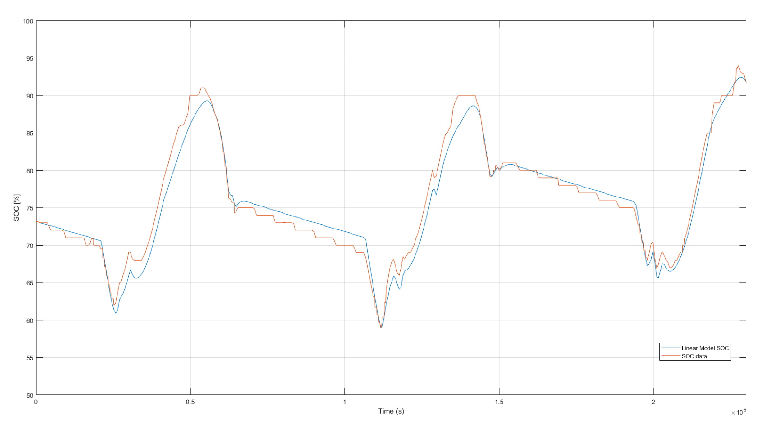
Figure 6 shows a comparison between the measured data and computed one. The inputs of the model are the profiles of $P_{SOL}$ and $P_c$ measured online with the system inverters, depicted in Figure 7.

2.3.2. Battery Degradation

Degradation is one of the main disadvantages of this electrochemical ESS. In the case of microgrids, the estimated lifetime of the battery is lower than that of the other elements of the system, thus, the maintenance and renovation of the battery system is a crucial cost of the microgrid. With this premise, it seems reasonable to include the battery degradation as one of the criteria to be minimized.

The rate of capacity loss is a complex nonlinear process dependent on factors as the state of charge (SOC), temperature, depth of discharge (DOD), discharge rate, time, and the environmental conditions of the battery [35]. In this work, it is assumed that the temperature and environmental conditions of the battery cannot be modified, as they are stored in a temperature-controlled room, thus, these factors will not be taken into account.

With this assumption, the concept of Ah-throughput can be used to estimate the battery’s lifetime [36]. Ah-throughput represents the quantity of charge delivered by the battery. It is expected that there is an amount of Ah-throughput that can circulate through the battery before it reaches the end of lifetime (EOL) [37].

In order to understand the concept of Ah-throughput it is necessary to introduce two new variables:

• $C_{rate}$: The ratio between the battery current and its nominal capacity;

  $$C_{rate}={\displaystyle \frac{|I_{BAT}|}{C_n}}$$

  (16)
• Depth of Discharge (DOD): The complementary of the SOC.

  $$DOD=100-SOC$$

  (17)

The nominal current of the battery $I_{nom}$ is the current produced if the battery is charged/discharged with a $C_{rate}=1$, depth of discharge of $DOD=100\%$, and temperature of $25°$C. Then, the nominal Ah-throughput of a battery is defined as:

$$A{h}_n={\int }_0^{EOL}\left|I_{nom}\right|dt.$$

(18)

For an arbitrary battery current, the effective Ah-throughput can be computed as:

$$Ah={\int }_0^{t_f}\left|I_{BAT}\right|\sigma dt$$

(19)

where $\sigma$ is the severity factor, which depends on the $C_{rate}$ and the DOD. In this study, the battery’s nominal capacity is large enough to assume that the $C_{rate}$ will always be below 2, hence the severity factor has a negligible effect and can be considered to be one [38].

Finally, the battery lifetime $B_l$ can be computed as,

$$B_l={\displaystyle \frac{Ah}{A{h}_n}}100[\%].$$

(20)

It can be observed that a reduction in the effective Ah-throughput can lead to an extension of the battery lifetime. Thus, a reduction in the charge/discharge currents $I_{BAT}$ requested to the battery can lead to a significant extension of the battery lifetime.

2.4. Hydrogen Generation Facility

The variability and unpredictability of the solar energy source might be compensated with a battery system, which stores the energy excess of high irradiance hours and supplies it to the loads in low irradiance hours. However, in some conditions, the solar inverters might have to reduce the generation of electrical energy. For example, when the generation exceeds the energy demand and the battery bank is too stocked to store it. This generation reduction is a direct energy loss that has to be avoided. For this reason, it is convenient to have an auxiliary system that can utilize this energy surplus.

In the scenario under study [18,39], there is a facility that generates hydrogen in order to refuel a fuel cell hybrid electrical vehicle. The main element of this subsystem is an alkaline electrolyser ACTA EL-500, which produces hydrogen through the electrolysis of water. When conditions of energy excess and high battery’s SOC are faced, the energy management system turns on the hydrogen facility so solar energy is not wasted. However, in some cases, it is advantageous to start the hydrogen production before these conditions are met. For this reason, further optimization can be achieved if the hydrogen scheduling problem is solved with the predictive approach.

The hydrogen facility will be modeled as an ON/OFF system. In the state ON the hydrogen facility will demand the operational power of its components. In the state OFF, the hydrogen facility will be supplied with a fraction of the electrolyser operational power, as too low energy supply may create hazardous conditions for the alkaline electrolyser. Therefore, the hydrogen facility is always supplied with some energy. The difference between an active hydrogen facility (state ON) or inactive (state OFF) is the amount of energy demanded. The activation of the hydrogen facility will be a controllable input of the microgrid.

3. Control Problem

3.1. Introduction

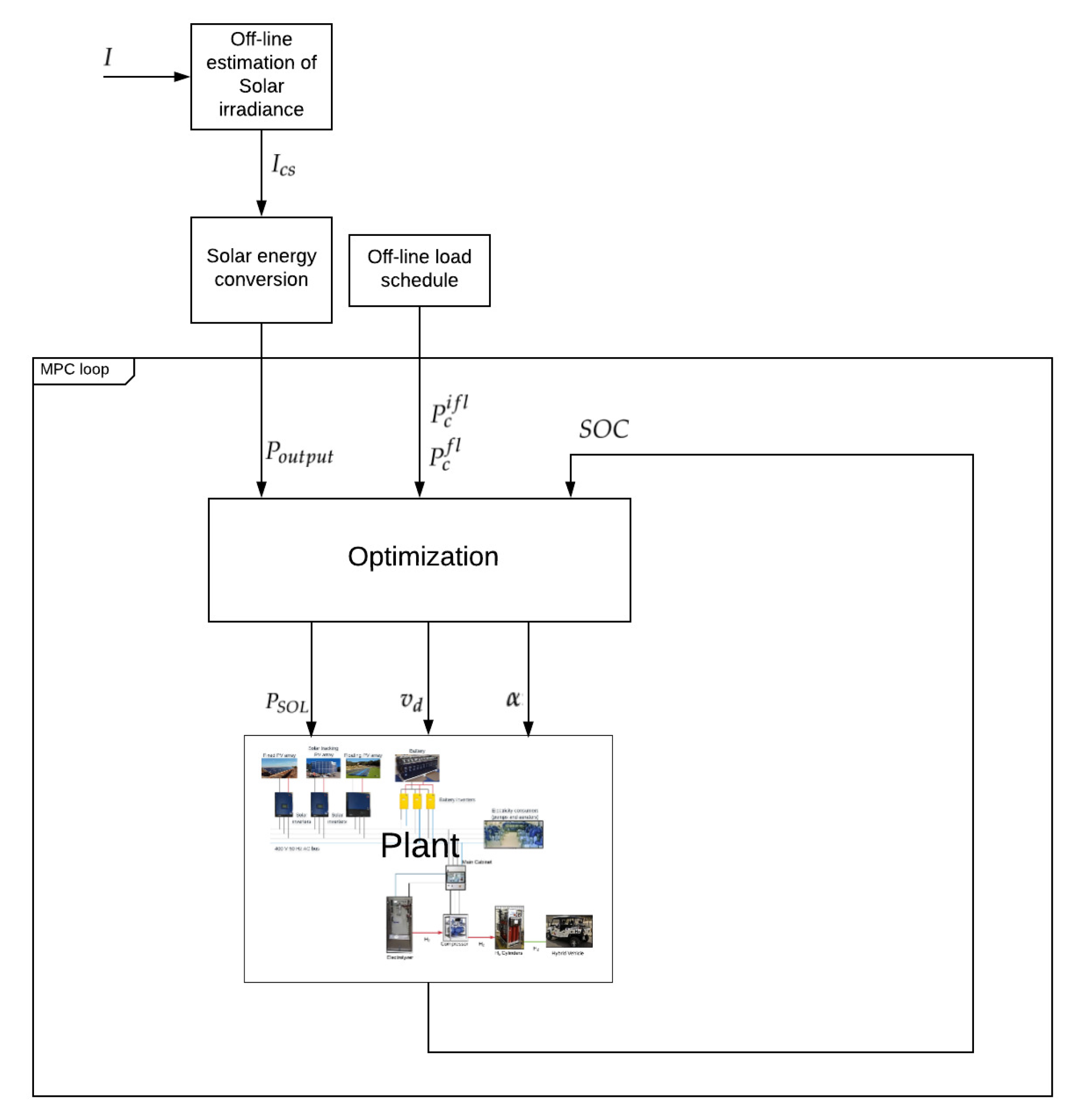
For the formulation of the control problem, it is convenient to define the controllable inputs and the measured variables needed by the controller. Accordingly, the controllable inputs can be characterized as follows:

• $P_{SOL}$: Real variable depicting the electrical energy introduced to the system through the inverters of the solar panels. Note that this variable will be bounded by the available solar energy;
• $v_d$: Binary signal that activates the time flexible load d. The loads that are time inflexible will not be governed by the controller of this work;
• $\alpha$: Binary signal that governs the activation of the hydrogen facility.

In order to compute the control action, the controller needs to have some knowledge about the state of the system. In this work, the controller requires information about the batteries’ state of charge. Moreover, in order to estimate the solar irradiance ($I_{cs}$), it is necessary to compute the daily mean of the atmospheric turbidity ($T_{L,n-1}$). This computation involves the measure of solar irradiance (I). Finally, the MPC requires the knowledge of the loads schedule, $P_c^{fl}$ and $P_c^{ifl}$. In Figure 8, the general control scheme can be seen.

Model predictive control (MPC) is a well-known control strategy that has proven to provide positive results in applications where tight performance is needed under several process constraints [40]. The main concept of MPC is to use a model to predict the behavior of the system and then apply an optimization technique in order to determine a control action that enhances the predicted behavior [41]. In predictive schemes, at each time step, the current control input is found by solving a finite horizon optimization problem.

The main elements of the MPC are the model used to compute the predictions, the cost function to be minimized, the process constraints to be satisfied, and the prediction horizon of the optimization. All the MPC’s decision variables and parameters to be used are summarized in

Table 2. Description of the model predictive control’s (MPC) decision variables and parameters.

Continuous decision variables
$P_{SOL}$	Electrical output of the solar panels controlled by the inverters
Binary decision variables
$v_d$	Variable denoting the activation of load d
$\alpha$	Variable denoting the activation of the hydrogen facility
$z_d$	Variable denoting that the flexible load d is active
b	Variable denoting the charging of the battery
Parameters
D	Power demand of the flexible load
L	Minimum consecutive active time intervals of the flexible load
$T_0$	Scheduled activation time of the load
$Sl$	Maximum time intervals that the flexible load can be advanced/delayed
${\overline{P}}_{BAT}$	Maximum battery charge/discharge power
$\underline{SOC}/\overline{SOC}$	Maximum/minimum allowed state of charge

.

3.2. Cost Function Definition

The MPC’s algorithm aims to minimize the cost function with the proper selection of the control action. Hence, the cost function has to be a description of the desired control objectives, which, in this work, can be defined as follows:

• To ensure that the demand of the system can be afforded;
• To maximize the production of $H_2$ from the hydrogen facility;
• To avoid actions that can damage the battery system.

The first control objective is considered to be mandatory and for this reason it will be introduced as a hard constraint instead of a term of the cost function.

The rest of the control objectives will be directly included in the cost function:

• Large discharge rate of the battery is one of the main factors that contributes to its degradation, due to this, the following term will be included:

  $$J_1\left(k\right)={\left(P_{BAT}^{dch}\left(k\right)\right)}^2;$$
• Maintaining the batteries around a reasonable SOC is crucial to ensure the uninterrupted supply of the power to the scheduled energy consumption. To accomplish this the following term is included:

  $$J_2\left(k\right)={(SOC\left(k\right)-\overline{SOC})}^2,$$

  where $\overline{SOC}$ corresponds to the reference value.
  In cases where the microgrid is not self-sufficient, the reference value $\overline{SOC}$ may not be trackable by just the RES generation and it may be necessary to exchange energy with the grid. In such cases, the viability of the control scheme can be studied through indicators such as energy-independence and self-supply [39,42], which could be optimized by adding an additional term in the cost function that penalizes the exchange with the grid [39];
• To maximize the production of hydrogen, the following term is considered:

  $$J_3\left(k\right)=-{\left(\alpha \left(k\right)\right)}^2.$$

All these terms will be combined in the cost function as:

$$J\left(k\right)=c_1{J}_1\left(k\right)+c_2{J}_2\left(k\right)+c_3{J}_3\left(k\right),$$

(21)

where $c_1$, $c_2$ and $c_3$ are three weighting terms to be fixed.

3.3. Characterization of Time Flexible Loads

Some loads could be described as time flexible, meaning that they can be advanced or delayed from the scheduled time [18]. In this work, it is considered that the consumption of the aerators of the wastewater treatment system can be shifted in time. This flexibility can be used to readjust the load schedule to the variability of renewable supply, which may result in a reduction of the size and use of the battery system.

In the following, how these loads can be modeled in order to introduce them in the optimization problems will be described.

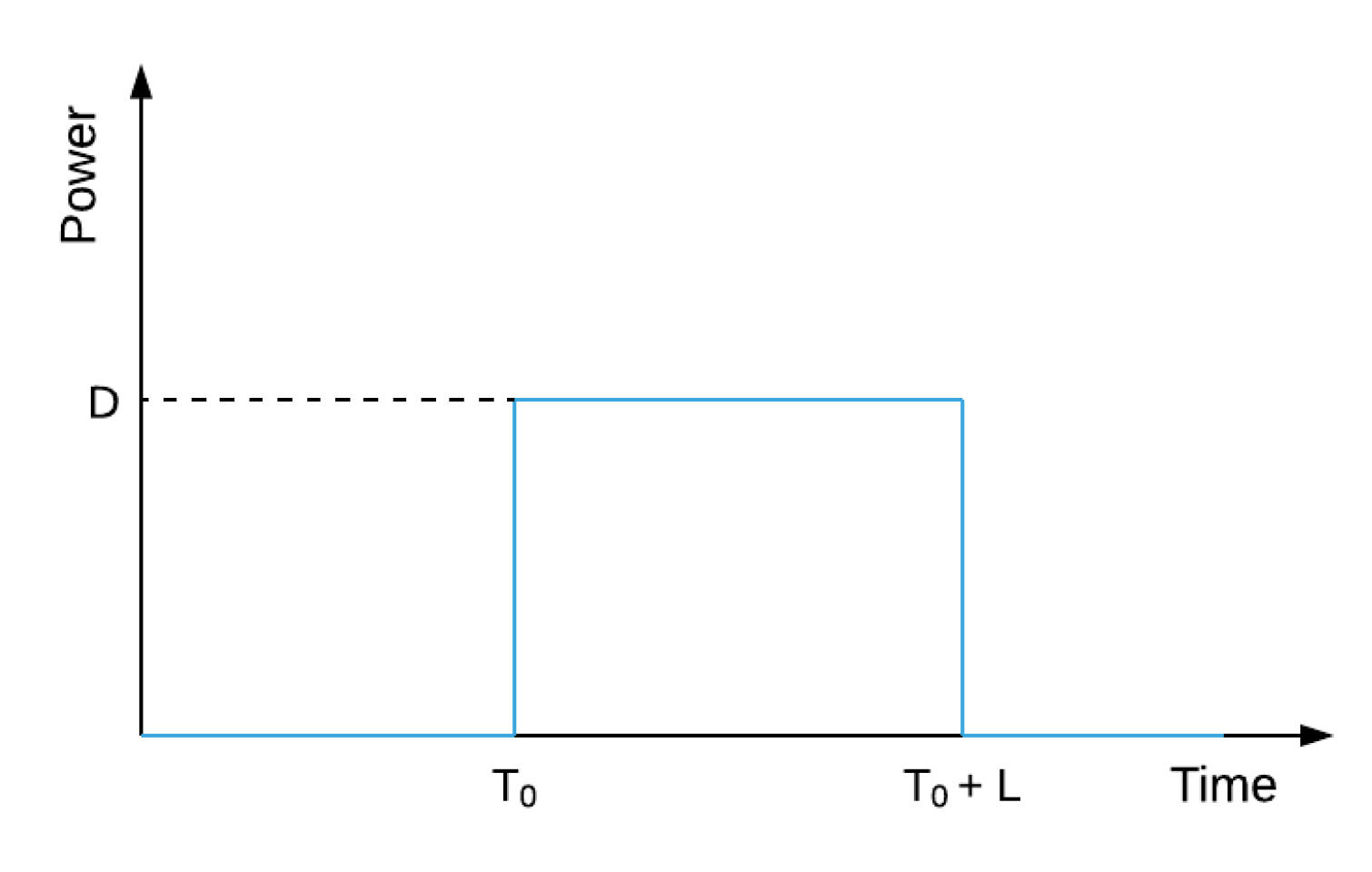
An energy load can be characterized by a constant power demand D that has to be supplied during a minimum of L consecutive sampling time intervals, from a scheduled starting time, $T_0$, to an end time, $T_0+L$, depicted in Figure 9. In other words, they can be advanced or delayed some time from the scheduled starting time, $T_0$. Note that only the starting time is modified, the minimum duration, L, remains invariant. Hence, a consumption load advanced n time intervals would start at time $T_0-n$ and end at $T_0-n+L$.

Time flexibility is acknowledged to be bounded, thus, consumption loads can be advanced or delayed to a maximum of $S_l$ time intervals.

This formulation, in contrast to the one of the time inflexible loads, does not define a unique solution, as the consumption load can start at any sampling time $k\in \{T_0-S_l,T_0+S_l\}$. Hence, the system flexibility is increased and a further optimization can be achieved.

The load will be represented as signal $P_c^{fl}\left(k\right)\in {\mathbb{R}}^{+}$ which can take two values, 0 if the load is not active and $D\in {\mathbb{R}}^{+}$ if it is active. In order to transform in terms of binary variables it is rewritten as :

$$P_c^{fl}\left(k\right)=z_d\left(k\right)·D\forall k,$$

(22)

where $z_d\left(k\right)\in \mathbb{B}$ are binary variables which will be defined over the optimization procedure.

In order that $P_c^{fl}\left(k\right)$ fulfills the desired characteristics different constrains will be defined over the binary variables $z_d\left(k\right)$:

(1)

To guarantee that $P_c^{fl}\left(k\right)$ is active in the interval $\{T_0-S_l,T_0+S_l\}$ it is necessary to fulfill that :

$$\mathbf{Constraint}\mathbf{1}:\sum _{k\in \{T_0-S_l,T_0+S_l\}}^{}{P}_c^{fl}\left(k\right)\ge E_d$$

(23)

where $E_d$ is a constant parameter that can have any value bounded to $0<E_d<D$;

(2)

To force that $P_c^{fl}\left(k\right)$ starts in some time $k\in \{T_0-S_l,T_0+S_l\}$ the following condition is also considered:

$$\mathbf{Constraint}\mathbf{2}:P_c^{fl}\left(k\right)-P_c^{fl}(k-1)\le T_{sl}\left(k\right)D\forall k$$

(24)

where $T_{sl}\left(k\right)\in \mathbb{B}$ equals 1 if $k\in \{T_0-S_l,T_0+S_l\}$, otherwise, $T_{sl}\left(k\right)=0$;

(3)

Finally, to ensure that $P_c^{fl}\left(k\right)$ remains active at least L consecutive time intervals the following constrain is required:

$$\mathbf{Constraint}\mathbf{3}:\sum _{k-L}^k{v}_d\left(k\right)\le z_d\left(k\right)\forall k,$$

(25)

where $v_d\in \mathbb{B}$ is a binary variable that is equal to 1 if and only if $z_d\left(k\right)-z_d(k-1)=1$. This is usually implemented including the additional constrain:

$$\mathbf{Constraint}\mathbf{4}:v_d\left(k\right)\ge z_d\left(k\right)-z_d(k-1)\forall k.$$

(26)

3.4. Controller Formulation

The proposed controller will try to minimize the cost function defined in Section 3.2, during the system evolution. To do this, a MPC approach will the used and in this context the dynamic problem is transformed into an static one focusing in a finite horizon. To do this, the system behavior is rewritten as a set of constrain over the optimization. The first ones correspond to a discrete time version of the system dynamic, Equation (15):

$$\begin{array}{ccc}\hfill SOC\left(k\right)& =& SOC(k-1)+P_{BAT}\left(k\right)\hfill \end{array}$$

(27)

$$\begin{array}{ccc}\hfill P_{BAT}\left(k\right)& =& {\alpha }_{ch}{P}_{BAT}^{ch}\left(k\right)-{\alpha }_{dch}{P}_{BAT}^{dch}\left(k\right),\hfill \end{array}$$

(28)

where ${\alpha }_{ch}\in {\mathbb{R}}^{+}$ and ${\alpha }_{dch}\in {\mathbb{R}}^{+}$ represent charging and discharging efficiencies and $P_{BAT}^{ch}\left(k\right)\in {\mathbb{R}}^{+}$ and $P_{BAT}^{dch}\left(k\right)\in {\mathbb{R}}^{+}$ correspond to the charging and discharging battery powers. Secondly, a power balance constrain is included:

$$P_{SOL}\left(k\right)-P_{BAT}\left(k\right)-P_c^{ifl}\left(k\right)-P_c^{fl}\left(k\right)-P_{H_2}\alpha \left(k\right)=0$$

(29)

where $P_{SOL}\left(k\right)$ represents the electrical power coming from the photovoltaic inverters, $P_c^{fl}$ and $P_c^{ifl}$ represents the power from the flexible and inflexible loads respectively loads, $P_{H_2}$ represents the electrical power consumed by the electrolyser, and $\alpha \left(k\right)\in \mathbb{B}$ is a binary variable used to indicate if the electrolyser is turned on or off.

To guarantee the consistency in a previous formulation, it is assumed that the charge and discharge processes cannot occur simultaneously; hence, a complementarity constraint is introduced:

$$\begin{array}{ccc}\hfill b\left(k\right){\overline{P}}_{BAT}& \le P_{BAT}^{dch}\left(k\right)& \le b\left(k\right){\overline{P}}_{BAT}\hfill \end{array}$$

(30)

$$\begin{array}{ccc}\hfill (1-b\left(k\right)){\overline{P}}_{BAT}& \le P_{BAT}^{ch}\left(k\right)& \le (1-b\left(k\right)){\overline{P}}_{BAT}\hfill \end{array}$$

(31)

where ${\overline{P}}_{BAT}\in {\mathbb{R}}^{+}$ is the operational upper limit of power through the battery, and $b\left(k\right)\in \mathbb{B}$ is a binary variable necessary to obtain a linear complementary constraint. A part from that, some constrains are considered to ensure that all variables are inside the required ranges:

$$\begin{array}{ccc}\hfill \underline{SOC}& \le SOC\left(k\right)& \le \overline{SOC}\hfill \end{array}$$

(32)

$$\begin{array}{ccc}\hfill 0& \le P_{BAT}^{ch}\left(k\right)& \le {\overline{P}}_{BAT}\hfill \end{array}$$

(33)

$$\begin{array}{ccc}\hfill 0& \le P_{BAT}^{dch}\left(k\right)& \le {\overline{P}}_{BAT}\hfill \end{array}$$

(34)

where $\overline{SOC}$ and ${\overline{P}}_{BAT}$ denotes the maximum value of $SOC$ and $P_{BAT}$, respectively, and $\underline{SOC}$ denotes the minimum value of $SOC$.

The electrical energy generated by the solar panels is constrained by the available solar irradiance, which will be estimated with the irradiance model presented in Section 2.2:

$$0\le P_{SOL}\left(k\right)\le {\widehat{P}}_{SOL}\left(k\right)$$

(35)

where ${\widehat{P}}_{SOL}\left(k\right)$ is the estimated potential generation of solar electric energy.

Finally, it is necessary to include all the constraints related to the time flexible loads described in Section 3.3.

Combining the cost function, the free variables used to obtain the optimal solution, and the set of constrains previously introduced, the following optimization problem is formulated:

$$\begin{array}{c}\hfill {\displaystyle \underset{P_{SOL}\left(k\right),z_d\left(k\right),v_d\left(k\right),\alpha \left(k\right),b\left(k\right)}{min}=\sum _{k=1}^N{c}_1·J_1\left(k\right)+c_2\left(k\right)·J_2\left(k\right)+c_3·J_3\left(k\right)}\\ \hfill s.t.\\ \left.\begin{array}{ccc}SOC\left(k\right)\hfill & =\hfill & SOC(k-1)+P_{BAT}\left(k\right)\hfill \\ P_{BAT}\left(k\right)\hfill & =\hfill & {\alpha }_{ch}{P}_{BAT}^{ch}\left(k\right)-{\alpha }_{dch}{P}_{BAT}^{dch}\left(k\right),\hfill \end{array}\right\}\mathrm{System}\mathrm{dynamics}\hfill \\ \left.P_{SOL}\left(k\right)-P_{BAT}\left(k\right)-P_c^{ifl}\left(k\right)-P_c^{fl}\left(k\right)-P_{H_2}\alpha \left(k\right)=0\right\}\mathrm{Power}\mathrm{balance}\hfill \\ \left.\begin{array}{c}b\left(k\right){\overline{P}}_{BAT}\le P_{BAT}^{dch}\left(k\right)\le b\left(k\right){\overline{P}}_{BAT},\hfill \\ (1-b\left(k\right)){\overline{P}}_{BAT}\le P_{BAT}^{ch}\left(k\right)\le (1-b\left(k\right)){\overline{P}}_{BAT},\hfill \\ \underline{SOC}\le SOC\left(k\right)\le \overline{SOC},\hfill \\ 0\le P_{BAT}^{ch}\left(k\right)\le {\overline{P}}_{BAT},\hfill \\ 0\le P_{BAT}^{dch}\left(k\right)\le {\overline{P}}_{BAT},\hfill \\ 0\le P_{SOL}\left(k\right)\le {\widehat{P}}_{SOL}\left(k\right),\hfill \end{array}\right\}\mathrm{Operational}\mathrm{constrains}\hfill \\ \left.\begin{array}{c}\sum _{k\in \{T_0-S_l,T_0+S_l\}}^{}{P}_c^{fl}\left(k\right)\ge E_d\hfill \\ P_c^{fl}\left(k\right)-P_c^{fl}(k-1)\le T_{sl}\left(k\right)D\forall k\hfill \\ \sum _{k-L}^k{v}_d\left(k\right)\le z_d\left(k\right)\forall k\hfill \\ v_d\left(k\right)\ge z_d\left(k\right)-z_d(k-1)\forall k.\hfill \end{array}\right\}\mathrm{Flexible}\mathrm{loads}\hfill \end{array}$$

where N corresponds to the prediction horizon discussed in Section 3.5. The overall problem contains $3N$ decision variables, which are: $P_{SOL}\left(k\right)$ (real), $v_d\left(k\right)$ (binary), and $\alpha \left(k\right)$ (binary). It also contains N state variables, $SOC\left(k\right)$, and $5N$ auxiliary variables, $P_{BAT}\left(k\right),P_{BAT}^{ch}\left(k\right),P_{BAT}^{dch}\left(k\right),b\left(k\right),z_d\left(k\right)$. Finally, the problem contains $4N$ equality constraints and $(15+N-L+1)N$ inequality constraints. To address this problem optimization, a mixed integer linear programming is required.

3.5. Prediction Horizon

Adopting a suitable prediction horizon is crucial to obtaining interesting results. However, selecting the correct horizon is not an obvious problem. On the one hand, implementing a large prediction horizon can be very computationally costly, as the size of the optimization problem is proportional to the size of the horizon. Moreover, the accuracy of the prediction is compromised in the final time intervals of a large horizon, especially in the prediction of the solar irradiance. On the other hand, a small prediction horizon combined with unfavorable plant characteristics can easily drive the controller unstable [41].

In this work, a prediction horizon of 24 h, with a sampling time of 10 min, has been implemented. With this horizon, the value of the factor N would be 144.

3.6. Parameter Uncertainty and Robustness

Notice that the proposed control scheme is based on a deterministic representation of the microgrid. In a realistic scenario, some uncertainty on the model’s parameters should be expected. Due to the closed loop nature of the MPC scheme, the controller is expected to present certain robustness to small parametric uncertainty. Nevertheless, the presented model is sensitive to the forecasted parameters, i.e., the solar irradiation forecast and load consumption. The next section will show that, in the considered case scenario, the proposed MPC scheme achieves acceptable results. Nonetheless, the performance of the controller could be further improved by considering a robust MPC scheme. This type of controller can achieve solutions that remain feasible even if uncertain variables are changing, which has been shown to be really useful on similar power grids problems [43,44].

4. Results and Discussion

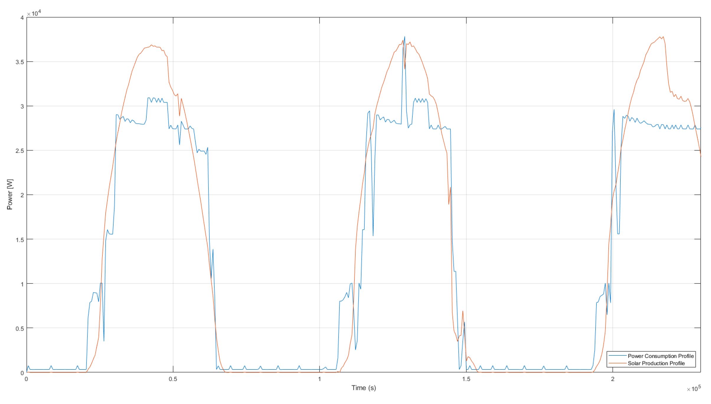
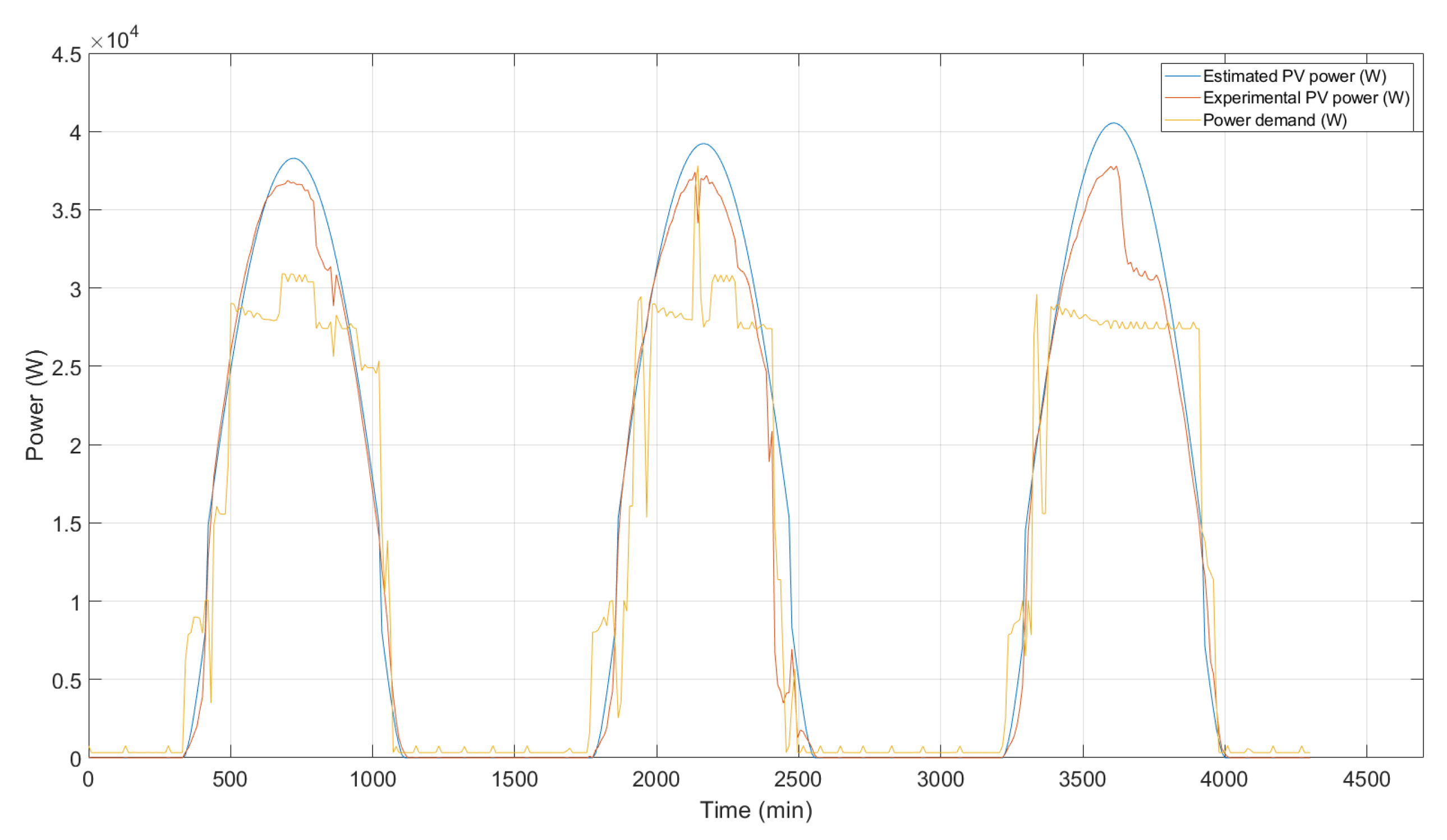
In order to evaluate the applicability of the proposed control strategy, different simulations have been performed. The simulation has been computed in MATLAB 2018a using the optimization software CPLEX studio 12.8 with an i7–8700K processor and 16 GB of RAM. Furthermore, the simulation starts at date 9 April 2016 , has a period of 72 h, and the predicted horizon is 24 h, which results in $N=144$. The system has been subjected to a profile of energy demand that has to be supplied by the photovoltaic panels. In order to introduce some disparity between the MPC’s estimation and the simulation, the system will be subject to an experimental profile of solar irradiance, using data measured at the panels pyranometer. In summary, three profiles have been introduced to the system: An energy demand profile, an estimation of available solar energy (used in the MPC’s computations), and an experimental profile of available solar energy (used in the simulation), which are depicted in Figure 10.

It is important to remark that the profile of energy demand depicted in Figure 10, is the summation of all the system’s loads, except the power supplied to the $H_2$ production. Furthermore, only one of the aerators (aerator 1) schedule can be advanced or postponed up to two hours from the scheduled time.

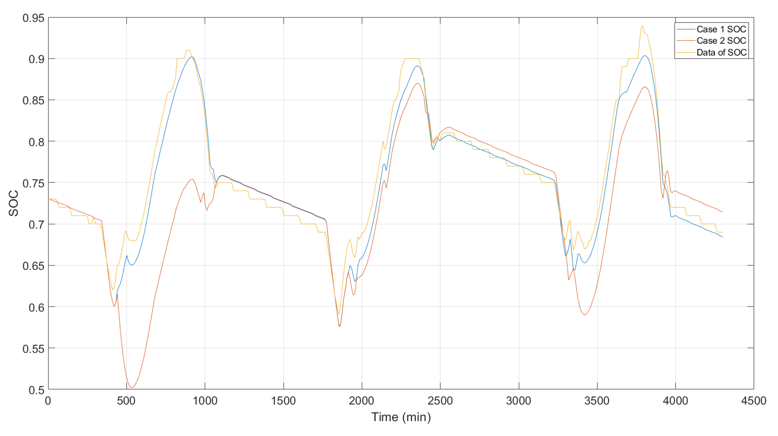
Moreover, experimental data of the battery’s SOC under the experimental profile of solar irradiance has been acquired. This data has been used to compare the results of the MPC’s energy management with the energy management implemented in [18]. Two cases have been studied and compared with the experimental data. In the first one, no production of hydrogen and no re-schedule of the aerator 1 load was allowed. With these conditions, the behavior of the system was very similar to the one without MPC. In the second one, the controller could re-schedule the aerator consumption and activate the hydrogen facility.

The results of the simulation have been the following. In the first case, the profile of PV energy introduced to the system (control input $P_{SOL}$) has been exactly the same as the experimental PV power of Figure 10, and the profile of energy demand has also been the same as the one presented in Figure 10. The evolution of the battery’s SOC has been very similar to the one depicted in the experimental data, represented in Figure 11.

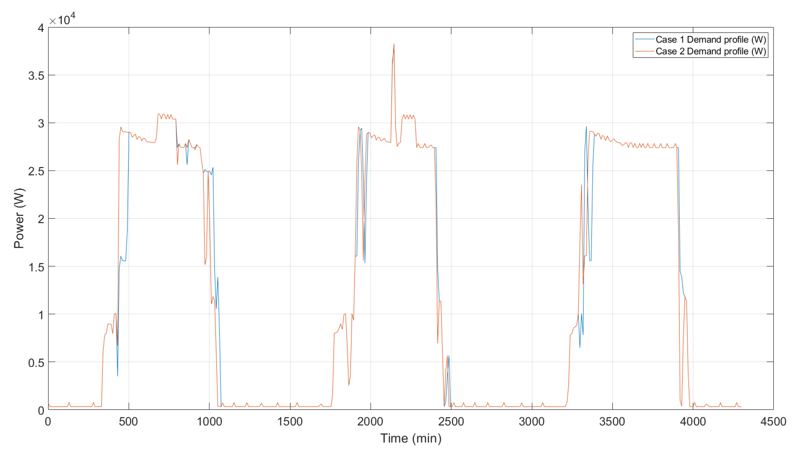
In the second case, the production of hydrogen and re-schedule of the aerator 1 load was allowed. Similar to the first case, the profile of PV energy introduced to the system (control input $P_{SOL}$) was identical to the experimental profile of available solar energy. However, some differences could be observed in the profile of energy demand, in Figure 12, and in the battery’s SOC profile, in Figure 11. On the first day, the load of the aerator 1 was advanced 60 min from its scheduled time. On the second day, the aerator 1 was advanced 10 min from its scheduled time. On the third, it was advanced 60 min from its scheduled time. This re-schedule of the loads produced a different evolution of the battery’s SOC, as depicted in Figure 11, and reduced its charge and discharge effort. A further explanation is included below.

In terms of the amount of energy cycled in the battery, in the first simulation case, the total amount of energy introduced and extracted was 180 kWh and 71 kWh, respectively. These values agreed with the experimental data. In the second case, a total amount of 177 kWh was charged to the battery (a reduction of 1.46%) and a total of 66 kWh was discharged (a reduction of 6.6%). These results show that the implemented MPC reduced the amount of energy cycled in the battery, compared to that obtained without MPC in [18]. This suggests that the inclusion of the MPC could reduce the size of the needed battery. This possibility could be taken into account when sizing the system [11], for instance, through simulation and optimization processes by genetic algorithms [9]. In this way, a reduction in the cost of the system and the energy produced was expected, similar to that obtained in [16].

It is noticeable that at the start and end of each day, the solar generation was lower than the energy demand and in consequence, a period of a fast discharge rate was requested to the battery. To reduce battery degradation, low SOC levels should be avoided. As can be seen in Figure 11, the re-scheduling of the time flexible load had reduced the discharge at the end of each day (912 min, 2355 min, and 3799 min) by increasing the discharge at the start of the day (441 min, 1900 min, and 3228 min). Moreover, the discharge increase at the start of the day was lower than the discharge reduction at the end of the day. As stated before, the charge of the battery was reduced by 1.46% and the discharge by 6.6%, therefore, the accumulated charge increased in the second simulation case. For this reason, the SOC’s value at the end of each day (1100 min, 2556 min, and 4000 min) was higher in case 2, as depicted in Figure 11, which was beneficial for the microgrid as the system became more robust to unexpected increases in system demand or unexpected reductions of the available solar energy. Furthermore, battery degradation, as well as operation and maintenance costs will be reduced [10].

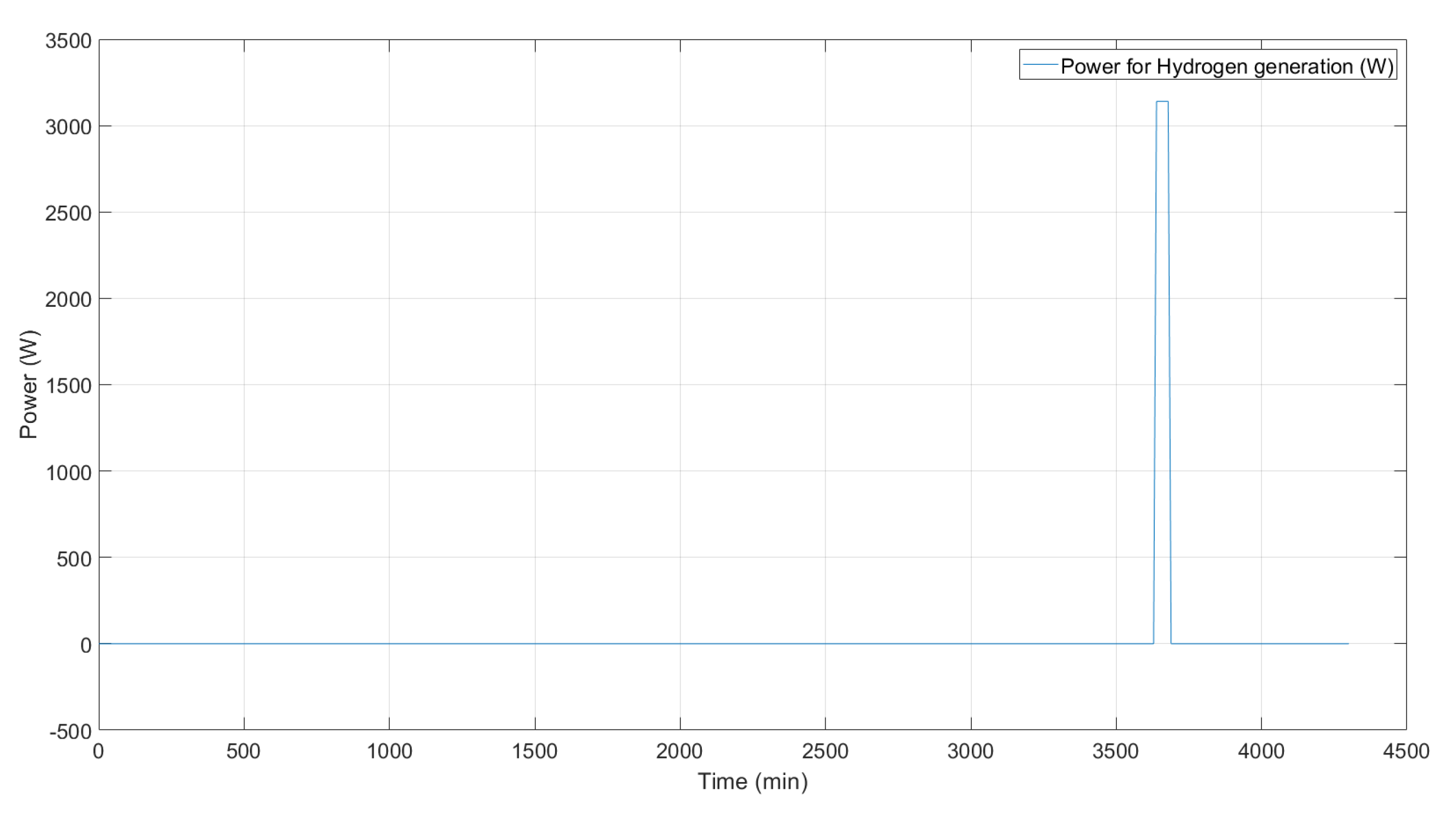
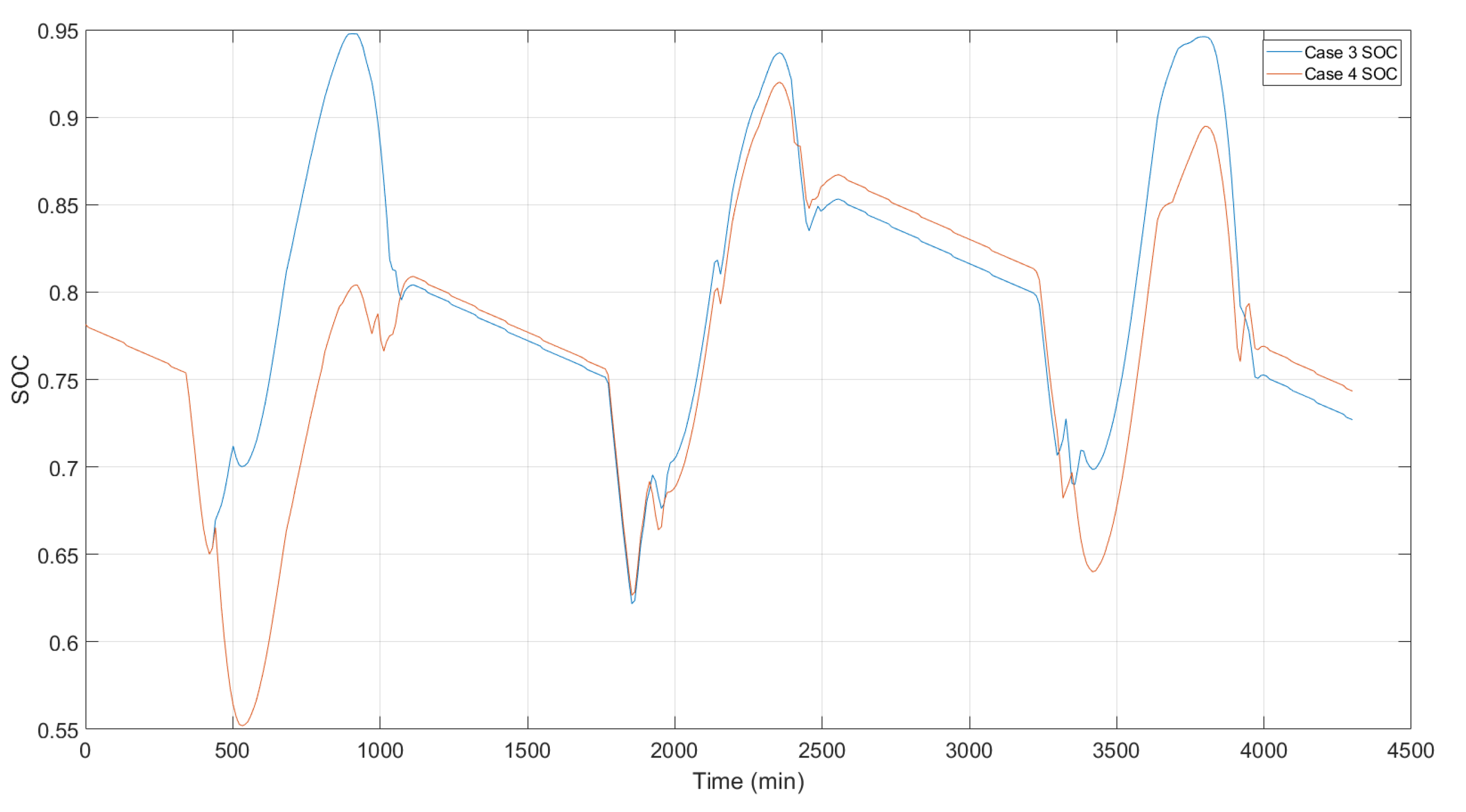
In both cases, and in the experimental data, there was no activation of the hydrogen facility. In order to evaluate the benefits of the controller in terms of hydrogen production, two more simulation cases have been studied. The simulations are exactly the same as the last ones (the first without the reschedule of the aerator 1 and the second with a reschedule) but, in this instance, the battery started with 5% more SOC. In the case where a re-schedule of the aerator 1 was allowed, there was an activation of the hydrogen facility, as depicted in Figure 13. The facility was switched on in the third day for a total duration of 50 min, which implies an approximate production of 417 Nl of hydrogen. It is remarkable that, even though the power consumption increased, the major benefits of the controller, in terms of reducing the battery’s effort, could still be observed as seen in Figure 14. In this sense, the incorporation of the MPC facilitated the deviation of the energy surplus for hydrogen production, alleviating the waste of energy that is usual in standalone fully based in renewable sources and non-dispatchable generation [5].

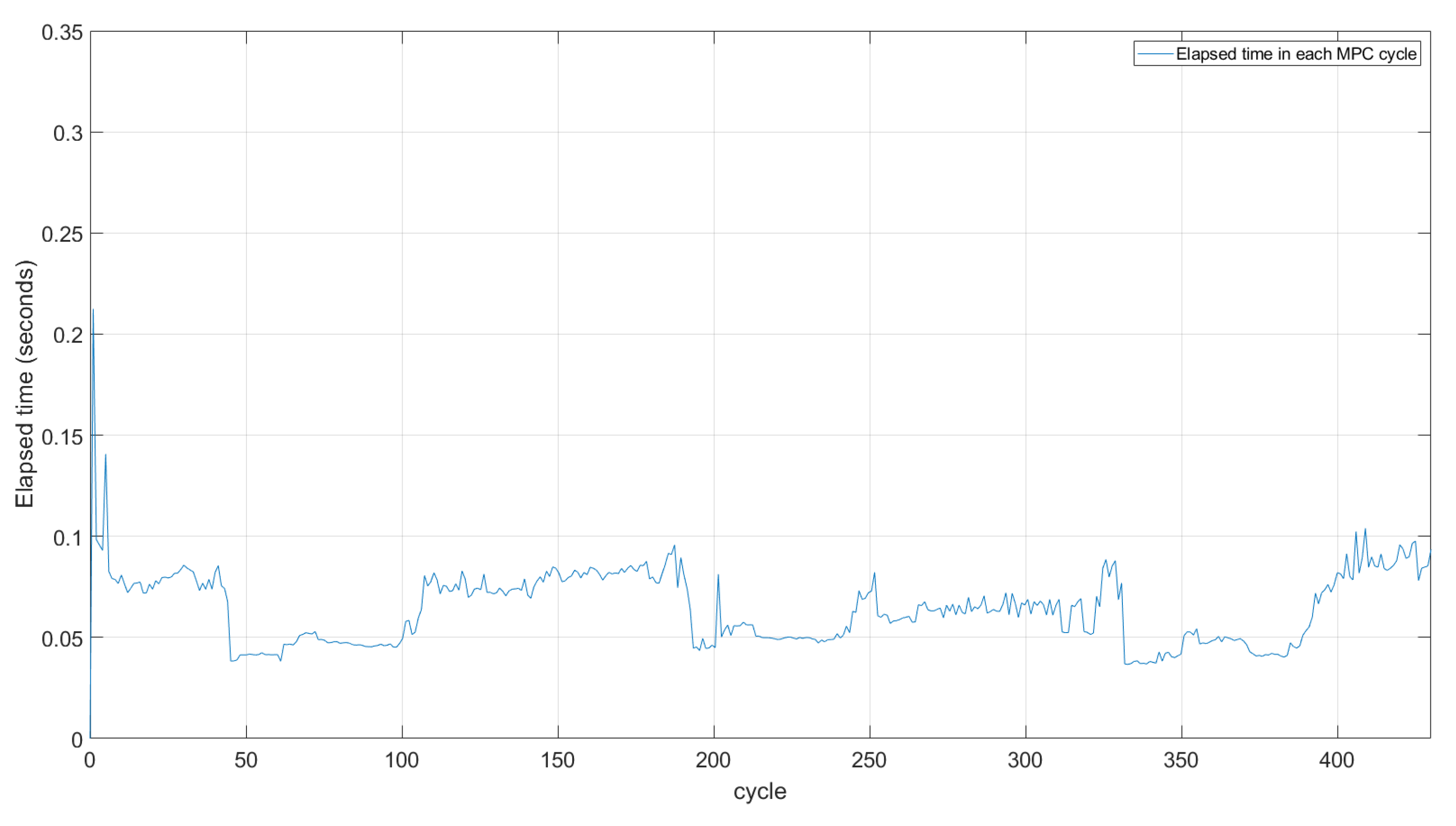
For the suitable operation of the MPC, it is crucial that the elapsed time between MPC cycles was lower than the sampling time considered. In Figure 15, it can be seen that the elapsed time in each cycle of the second simulation case was between 0.25 and 0.04 s. This time was lower than the 10 min considered as the sampling time, therefore, the controller will not present any conflict on this issue. The other simulation cases presented a similar elapsed time evolution.

5. Conclusions

In this paper, the application of a model predictive control for energy management in a standalone microgrid, whose only generation is photovoltaic, was presented. The results showed that the energy demand was managed through changes in the schedule of deferrable loads. It should be noted that, given the predictive nature of the control developed, the management of the loads was not limited to deferring them, but also to advance them. Thus, a reduction in the amount of energy cycled in the battery was obtained. In addition, the evolution of the battery SOC was stabilized, avoiding deep discharges. These results suggest that the implementation of the MPC could reduce the need for storage, prolong the life of the battery, and reduce the investment and operating costs of the system.

Regarding the simulations performed including the production of hydrogen, its activation occurred before the battery reached a very high SOC. This avoids wasting energy that can not be stored because the battery is completely full. In addition, when the system is sized, a smaller battery size could be chosen.

New work is required to quantify the advantages obtained. Future research includes the application of the proposed model predictive control to several case studies in order to quantify the benefits obtained in terms of battery lifetime, both on energy and system costs, and on the reduction of energy surplus. Experimental validation of the proposed predictive scheme must also be carried out. Moreover, the performance of the controller could be improved with the use of more accurate models of solar irradiance and the battery subsystem, and by the implementation of more complex control schemes such as the robust or stochastic variants of the MPC.