Abstract
New small-scale experiments are carried out to study the effect of groundwater flow on the thermal performance of water ground heat exchangers for ground source heat pump systems. Four heat exchanger configurations are investigated; single U-tube with circular cross-section (SUC), single U-tube with an oval cross-section (SUO), single U-tube with circular cross-section and single spacer with circular cross-section (SUC + SSC) and single U-tube with an oval cross-section and single spacer with circular cross-section (SUO + SSC). The soil temperature distributions along the horizontal and vertical axis are measured and recorded simultaneously with measuring the electrical energy injected into the fluid, and the borehole wall temperature is measured as well; consequently, the borehole thermal resistance (Rb) is calculated. Moreover, two dimensional and steady-state CFD simulations are validated against the experimental measurements at the groundwater velocity of 1000 m/year with an average error of 3%. Under saturated conditions without groundwater flow effect; using a spacer with SUC decreases the Rb by 13% from 0.15 m·K/W to 0.13 m·K/W, also using a spacer with the SUO decreases the Rb by 9% from 0.11 m·K/W to 0.1 m·K/W. In addition, the oval cross-section with spacer SUO + SSC decreases the Rb by 33% compared with SUC. Under the effect of groundwater flow of 1000 m/year; Rb of the SUC, SUO, SUC + SSC and SUO + SSC cases decrease by 15.5%, 12.3%, 6.1% and 4%, respectively, compared with the saturated condition.
1. Introduction
The ground source heat pumps (GSHP) systems become one of the leading technologies used recently worldwide to provide heating, cooling and domestic hot water (DHW) due to its privileges as a cost-effective operation and being environmentally friendly [1]. GSHP system consists of three main parts: a) the ground heat exchanger (GHX) which is absorbing/rejecting the heat from/to the subsurface layers of the surrounding soil; b) the heat pump (HP) is conveying the heat energy in bi-directional between fluid flowing through the GHX and the operating fluid from the building; c) the fan-coil system which transmits the heat energy to the desired space. The GHX could be horizontal or vertical types. The vertical GHX is extended deeply for more than 100 m underneath the soil surface, and it is preferred in a compact area as a high densely populated area [2]. However, high drilling cost is the main issue which is an obstacle preventing the wide spreading of it. On the other hand, horizontal GHX is extended in a horizontal plan, which requires a vast plan area, so it is not preferred in urban areas [3].
The thermal performance of GHX depends on several operating parameters, including inlet velocity, temperature and operating interval, and the hydrological composition of the surrounding soil [4]. In addition, accurate estimation of the soil thermo-physical properties (soil thermal conductivity, soil volumetric heat capacity and soil temperature distribution profile) leads to the proper design of the GHX dimensions. In-situ measurements by thermal response test (TRT) are the dominant common approach to determine these values and the borehole thermal resistance. The TRT methodology is injecting/extracting a constant rate of heat energy at a constant fluid flow rate inside BHX, and the inlet and outlet fluid temperature is recorded for continuous 48 hours [5,6,7,8,9]. The Infinite Line Source Model (ILSM) is the typical model to calculate and predict the soil properties; the LSM in an infinite homogenous medium, borehole and grouting is not accounted for in the ILS but is added through the borehole resistance term [10].
Moreover, the presence of groundwater advection can significantly enhance heat transfer and accelerate soil recovery state possibility [11]. Therefore, the thermal convection of the groundwater flow could impact the results calculated by the LSM [12]. Hence, many studies are recommended to perform multi TRTs at different places with different groundwater flow velocities, to assure accurate calculations of the soil properties and borehole thermal resistance [13,14,15,16,17,18,19,20,21].
Due to the high cost and long-time experimental effort of TRT, small-scale laboratory test and numerical simulation are of great importance for designing and predicting the performance of different configurations and designs of BHX. Examples of laboratory tests are: Li W et al. [22] investigated the effects of ground stratification on soil temperature distribution by an experimental apparatus with dimensions of 6.25 m × 1.5 m × 1m. Double Copper U-tube was buried horizontally inside a well-insulated box filled with sand and clay. Wan R. et al. [23] studied the effect of inlet water temperature, Reynolds number and backfilling material on thermal performance of a single U-tube heat exchanger. The single U-tube inserted inside a circular tank with diameter and depth of 240 mm and 1100 mm, respectively. Erol S. et al. [24] evaluated the performance of various grouting materials, through thermal, hydraulic and mechanical laboratory characterizations by sandbox with dimensions of 1 m × 1 m × 1m. Li H. et al. [25] investigated the effect of groundwater flow on the performance of spiral heat exchanger. Their experimental set-up consisted of a well-insulated stainless-steel box divided into three sections that were separated by a metal mesh and filter. The middle part was the test section, which had dimensions of 0.4 × 0.5 × 0.8. A spiral heater was filled with saturated silica sand to represent the spiral heat exchanger. Beier R.A. et al. [26] introduced a reference data set from a large laboratory “sandbox” containing a borehole with a U-tube. Their experimental measurements included thermal response tests on the borehole include temperature measurements on the borehole wall and within the surrounding soil. The test data provide independent values of soil thermal conductivity and borehole thermal resistance for verifying borehole models and TRT analysis procedures.
While numerical methods present another effective alternative with an acceptable accuracy to full-scale experimental tests. Computational fluid dynamics (CFD) approach can study the impacts of the diversity of factors on the performance of BHX with various configurations and arrangements [27,28,29,30,31,32,33,34,35,36]. For example, Jahangir MH et al. [37] utilized the classical finite element method to study the thermal and moisture behavior of the heat exchanger during the heat transfer process of several U-shape straight pipes. In addition, Biglarian H. et al. [38] developed a numerical model to simulate the short-term and long-term performance of the borehole heat exchanger. Their model simulated the fluid transport through the U-tube and the temperature variation of the borehole components with depth.
From this literature, the performance of ground heat exchanger under the impact of saturated conditions with groundwater flow was extensively investigated. Either by full scale experimental analysis or numerical simulations. All of these studies used the conventional costumery U-tube heat exchanger with a circular cross-section, no one tried to use an oval cross-section U-tube. The oval shape has many advantages over the circular tube as the author has shown in former research [39]. In this paper, the authors developed a new small-scale experimental set-up to compare the thermal performance of four different heat exchangers under the effect of groundwater flow. Finally, a two-dimensional, steady-state computational fluid dynamics simulation is carried out by ANSYS FLUENT software (ANSYS 2019 R3, Free student version, ANSYS INC, USA) to simulate and predict the soil temperature distribution, borehole thermal resistance and borehole temperature under different groundwater flow velocities.
2. Experimental Set-Up
A small-scale experimental set-up investigates the effect of groundwater flow on the thermal performance of GHX in laboratory scale. Comparison of the thermal performance of oval and circular cross-sections is carried out. The apparatus consists of 4 tanks (a, b, c and d) as shown in Figure 1. A comprehensive explanation about experimental set-up and instrumentations are indicated as follows:
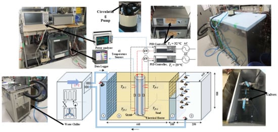
Figure 1.
Schematic diagram and pictures of the experimental set-up.
2.1. SandBox
The main test section (Tank B) is consisting of a double-wall stainless steel tank with dimensions of 400 mm x 500 mm x 800 mm, (W x L x H), the front and back walls thickness is 5 cm and filled with an insulation foam layer, while left and right walls are made from steel net and a semi-permeable membrane. The membrane is separating the sand and water interfaces; it permits the water to flow and prevents the sand particle to sweep into water tanks. The test section filled with wet silica sand and sand gravel filled the borehole at the middle of the tank.
2.2. Groundwater Flow
The water flows from tank A to tank C passing through the voids and pores of the sand and grouting material in tank B. The flow rate is depending on the head difference between the water level in tank A and tank C, also the permeability of sand and gravel domains followed the Darcy flow principle. The flow rate is measured in each test by measuring the volume of water in liters that permeated through the sand and gravel in one minute. The head difference is controlled using ten ball valves fixed at the interface between tanks C and D; it is distributed every 5 cm from top to bottom. The upper surface of the four tanks is covered and insulated by high-density polyurethane foam insulation panel of 5 cm thickness.
2.3. U-Tube Heat Exchanger
The U-tube heat exchanger is simplified by using two parallel PVC pipes (the pipes are provided by Inoac Housing and Construction Material, Co., Ltd., Nagoya, Japan), it is filled with tap water and blocked from the bottom end. Two different cross-sections, oval and circular, are used with dimensions as indicated in Figure 2. Additionally, two different spacing distances are investigated. A total of four cases are studied; a single U-tube with a circular cross-section (SUO), a single U-tube with an oval cross-section (SUO), a single U-tube with a circular cross-section and a single spacer with a circular cross-section (SUC + SSC) and a single U-tube with an oval cross-section and a single spacer with a circular cross-section (SUO + SSC). The tubes are inserted inside the borehole which is filled with sand gravel with an average particle diameter of 5.5 mm as shown in Figure 3.
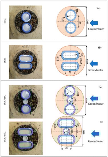
Figure 2.
Photos and dimensions of each case: (a) circle; (b) oval; (c) circle with spacer and (d) oval with spacer.
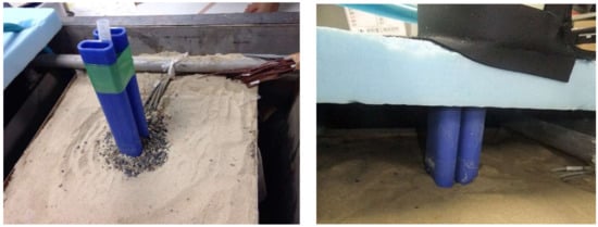
Figure 3.
Photos of U-tube inside the borehole and surrounding soil.
2.4. Initial Groundwater Temperature Measurements
The initial sand temperature is maintained at 15 °C using constant temperature water chiller (ADVANTEC LV 600, ADVANTEC INC., Tokyo, Japan). The chiller pump circulates the cold water through the sand pores in a closed loop circulation as shown in Figure 1. PT100 temperature sensor is inserted inside sand to controlling the temperature feedback to the chiller cooling circuit. After the temperature reaches the setting temperature, the chiller cooling circuit is switched off. While, the circulating pump remains working to keep the water level in tank A at the determined level.
2.5. Fluid Temperature Difference
The temperature difference between fluids inside the right and left tubes is 3 °C. It is controlled using two orders made heaters with a maximum heating power of 350 W. The two heaters are consisting of the heating element in the core made from NCHW1 (Nickel Chromium Wire, 80% Nickle, 20% chromium), the wire is insulated by Magnesium oxide powder, and it is shielded by an Aluminum layer. The heating element had dimensions of 860 mm × 9.45 mm × 5.9 mm (length, width and depth).
The input electrical power is controlled and regulated by a handmade proportional-integral-derivative (PID) controller circuit. The PID controls and regulates the input electrical power with a feedback signal from temperature sensor inserted inside the tube. The PID controller circuit consists of PID controller (Omron E5CK, OMRON Corporation, Kyoto, Japan) with sampling accuracy of 100 ms, circuit breaker (MCB1, C 10A), solid-state relay (TOHO TRS 1225, TOHO INC., Tokyo, Japan) and fuses 15 A.
Two small centrifugal electrical pumps (0.4 L/min and 10 W) are used to circulate water inside each tube to guarantee a uniform fluid temperature along the pipe length.
2.6. Instrumentations
2.6.1. Soil Temperature Measurements
Forty thermocouples measure the soil temperature (Type-T, red cross x), it is divided into two groups; each group containing 20 sensors which are divided into two levels at heights of 50 cm and 80 cm from the bottom, each level is distributed as shown in Figure 4. The first level at a height at 50 cm contains sensors from Ts1-1 to Ts1-20, while the second level at a depth of 80 cm contains sensors from Ts2-1 to T2-20. The borehole temperature is measured by four PT100 (blue circle), they are fixed at the mid plan and distributed counterclockwise from Tb1 to Tb4 as shown in Figure 4. The fluid temperatures are measured by four PT100s (green circle), each tube has two sensors at upper and lower parts. Before the sensors are fixed to the experimental set-up, they had been calibrated against a standard thermometer measurements in the temperature range between 15.25 °C to 30.2 °C and a temperature step of 5 °C by means of constant temperature water bath. The errors absolute and relative values for a sample of these PT100 temperature sensors and the average error value of the thermocouples are indicated in Table 1. Finally, 48 temperature sensors are connected to a data logger (Yokogawa DX2048, YOKAGAWA Electric, Tokyo, Japan) which has a sampling interval every 1 min.
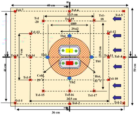
Figure 4.
Temperature sensors positions and section A-A and B-B for horizontal and vertical orientation.

Table 1.
Typical error of the PT100 temperature sensors and thermocouples.
2.6.2. Heating Rate Measurements
The electrical power supplied to each electrical heater are measured by measuring the electrical current and voltage. The electrical current is measured by clamp on sensor (Hioki 9272). The electrical voltage and current measurements are recorded and analyzed by power analyzer (Hioki 3390).
2.7. Physical, Thermal and Hydraulic Properties
The thermophysical properties of both soil and gravel are measured according to the associated standard. The Particle size distribution (PSD), porosity, thermal conductivity and heat capacity are measured and used in the numerical simulation.
a) Particle-size distribution and porosity
The particle-size distribution (PSD) is measured by the mechanical method according to ISO 13503-2, the sand/gravel sample is dried and weighted. Then it is shacked carefully to pass through a series of sieves with a coarse sieve at the top and finest one at the bottom. From measuring the weight percentages of sand/gravel retained in each sieve, then plotted against the sieve size, as shown in Figure 5a,b. This figure shows that the sand particle size is in the range of 150–300 μm, while the gravel size ranged from 2.8 mm to 5.6 mm.
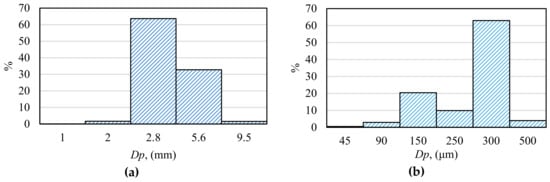
Figure 5.
Particle Size Distribution of: (a) Gravel and (b) Sand.
In addition, the porosity of both sand and gravel are measured following the standard method, the porosity (n) are 0.4 and 0.36 for sand and gravel when tightly packed, respectively.
b) Thermal conductivity
The thermal conductivity of sand and gravel is measured by the method of thermal response test analysis under dry and saturated conditions. The thermal conductivity, including the conductivity of solid grains and the pore-filling material. The measurements rely on a one-dimensional conduction test using the needle probe method. The experiment set-up includes the packing tube, with a length of 25 cm and a diameter of 5 cm, which is packed tightly with solid grains, then a needle heater with a length of 15 cm is inserted inside the porous material. A PT-100 thermocouple is integrated with the needle heater to measure the soil temperature gradient. The electrical voltage (V, [volt]), current (I, [Ambers]) and soil temperatures are measured and recorded via data logger as shown in Figure 6. The time step is 30 sec, and each experiment lasted for 10 minutes. Then, a linear relationship between temperature and log scale of time is derived. Then heating power (P, [W]) and the thermal conductivity (λ, [W/m·K] are calculated according to Equation 1 and Equation 2:
where P is the heating rate in W, H is the tube length in m and k is the slop coefficient
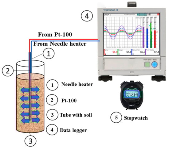
Figure 6.
Thermal conductivity measurement schematic diagram.
3. Error Analysis
The borehole thermal resistance calculations are affected by the error in the measurements of primary variables. The primary variables include the hot and cold fluid temperatures, borehole temperatures, soil temperatures and electrical voltage and current values. Improperly calibrated sensors, sensor installation and connections cause errors in these measurements. Therefore, error analysis is essential to clarify the error values in the desired calculated results—heating power and borehole thermal resistance. The following equations are applied to calculate the error values and percentages.
3.1. Error in Thermal Conductivity Measurements
The error of the thermal conductivity depends on the error of temperature measurement slop coefficient, heating power measurement and the tube length measurement and how these errors are combined according to Equation (1). The error values of P and λ are calculated by Equation (3) and Equation (4) with the reference values and error values listed in Table 2.
where V and I are the voltage and current values, are the error values in voltage and current, respectively.
where is the error value on heating rate in W, is the error value in tube length in m and is the error value of the slop coefficient.
Table 2.
Thermal conductivity and error % of sand and gravel in W/m.K.
3.2. Error in Heating Power Measurement
Two electric heaters are injecting heat to the surrounding fluid to keep the temperatures inside the two tubes at 32 °C and 29 °C respectively and maintain the temperature difference at 3 K. the current I (Ambers) and voltage V (Volt) are measured and recorded simultaneously and the electric power P (W) of each heater is calculated, then the heating rate per unit length q’ (W/m) are calculated as follows
where P is the total heating power of the two heaters in W
The error % values in q’ is calculated as shown in Equation (6):
Also, P and q’ are the heating power and heating power per unit length, while are the error values of heating power and heating power per unit length, respectively.
3.3. Error in Borehole Thermal Resistance Calculation
The borehole thermal resistance is calculated by the following equation:
The error value of the Rb is calculated as follows:
where Tf, Tb and q’ are the fluid temperature, borehole temperature and heating power per unit length, respectively. In addition, are the error values of temperature difference between fluid temperature and borehole temperature and heating rate per unit length, respectively. Table 3 listed the error percentage of these variables.
Table 3.
Error values of different variables and Rb.
4. CFD Simulation Set-Up
A two-dimensional finite volume model is developed by ANSYS FLUENT environment, the conjugated fluid flow and energy is solved simultaneously at a horizontal plane. The geometry is consisting of four domains for water filling left and right tanks (tanks 1 and 3), grout material inside borehole and sand filling the outer volume. The soil and gravel material are considered as porous media with the corresponding porosity and particle diameter. The following assumptions are applied in this study:
- The simulation is done under steady-state condition
- The ground water flow is considered as laminar flow through the porous voids
- Temperature independence of the solid materials’ properties (density, thermal conductivity and specific heat capacity).
- The gravitational force effect was not considered.
- a.
- The fluid volume is omitted, and the tube inner wall temperature had been set at the same fluid temperature
- The soil and borehole are considered as homogenous porous in all directions.
The governing equations controlling the heat transfer and mass transfer through the porous voids inside the grout and sand materials are shown in the following subsections:
a) Mass conservation equation
The mass conservation equation or “continuity equation” Equation (9 is written as follows:
where is fluid density in (kg/m3), is velocity vector in (m/s)
b) Momentum conservation equation
The general form of the momentum equation inside porous media is the standard fluid flow equation with additional momentum source term
where is the static pressure in (N/m2), is the surface shear stress in (N/m2), is the gravitational body force in (N/m3) which is neglected in this study, is the external body force in (N/m3) and is the momentum source that is calculated by Equation (11)
The first term in Equation (11) is the viscous term and the second term is the inertia loss term. Where is the source term for the th momentum equations (. is the permeability and C2 is the inertia resistance factor calculated by Equation (12) and Equation (13), respectively.
where, Dp is the particle size (m), while is the porosity.
In laminar flow, the momentum sink creates a pressure drop through the porous media, is the pressure drop is proportional to the velocity as indicated in Equation (14)
where is the fluid viscosity (kg/ms) and is the velocity vector.
c) Energy conservation equation
The energy equation for porous media is a blending between the energy of the fluid and the solid, the blending factor is the porosity. In fluent, the standard energy transport equation is modified by include the effective conductivity and the thermal inertia of the solid region on the medium as shown in Equation (15)
where is the effective thermal conductivity in the porous medium and it is calculated by Equation (16)
where and are fluid phase and solid medium thermal conductivity, respectively.
A two-dimensional simplified geometry is considered as shown in Figure 7a. The left and right water tanks are considered as a fluid domain, while the soil and the borehole are assigned as a porous medium with water as the continuum medium. The dimensions are corresponding to the exact experimental dimensions.
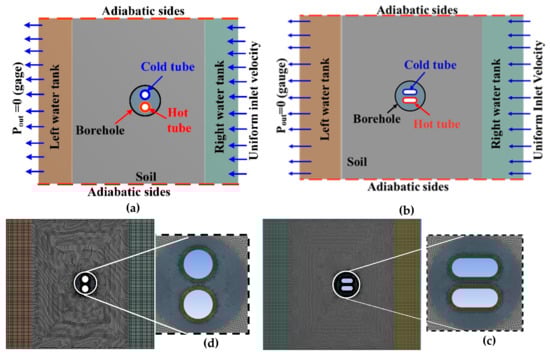
Figure 7.
Geometry and boundary conditions used in this study: (a) Geometry of single U-tube with circular cross-section (SUC); (b) geometry of ), single U-tube with an oval cross-section (SUO); (c) mesh of SUC and (d) mesh for SUO used in this study.
4.1. Mesh Independence Test
As seen in Figure 7b, structured mesh is discretized in the fluid domains of both inlet and outlet storage tanks. While the unstructured element is selected for the porous zones including the sand zone and the borehole zone. To confirm that the results are not dependent on the grid size, a mesh independence test was conducted. The mesh test results indicated that increasing the number of elements more than 27,000 has negligible impact on the simulation accuracy. Therefore, this number of elements were adopted through this study.
4.2. Boundary Conditions
In the present simulation, the right and left edges were defined as a velocity inlet and pressure outlet boundary condition, respectively. The velocity inlet changes from 0 (Saturation condition), 100 m/year, 300 m/year, 500 m/year and 1000 m/year. While the other outer edges are considered as adiabatic boundary as the outer surfaces of the experiment apparatus are perfectly insulated. The groundwater flows from the right water tank through the porous media to the left water tank with a constant inlet temperature of 16 ± 0.5 °C. In addition, the initial temperature of 16 ± 0.5 °C is patched for all domains.
4.3. Solver Schemes
In this study, the fluid flow and temperature distribution were solved by couple arithmetic, while a second order discretization scheme was used to discretize pressure, X-momentum, Y-momentum, Z-momentum and energy equation. The convergence criteria are 10−3 for all equations except 10−6 for the energy equation.
5. Results and Discussions
A new small-scale laboratory test is built to investigate the impact of groundwater flow on the thermal performance of the ground heat exchanger with a unique oval cross-section. Four different configurations are investigated under the effect of groundwater velocity of 1000 m/year. The soil temperature distribution on a horizontal plane at a depth of 0.5 m, the fluid temperatures and heating injection rate are measured and recorded instantaneously. Simultaneously, two-dimensional and steady-state CFD simulations are validated against the experimental measurements. After validating the CFD model, it is used to compare the thermal performance of oval and circle cross-sections under different groundwater velocities. Four different cases have been studied, the cases are circle and oval shapes, and another two cases with a spacer. Furthermore, the borehole thermal resistances are calculated and compared.
The experiments were conducted for one week, and each experiment continues for seven hours, followed by twelve hours without heating. This period is needed for complete recovery of the soil temperature. In addition, the initial soil temperature, the hot and cold water temperatures and groundwater flow rate are controlled as possible to maintain the same values for all cases, but unfortunately, there is a bit fluctuation in the operating conditions from one case to another as listed in Table 4.
Table 4.
Experimental operating conditions and standard deviation (SD) in temperature and heating rate.
5.1. Experimental Results
5.1.1. Soil Temperature Contours
The soil temperature distribution contours for each configuration are drawn from the temperature measurements on a plane at a depth of 0.8 m, as shown in Figure 8. Figure 8 concluded that heat energy is advected by the effect of groundwater flow from right to left. Hence, the soil temperature at the upstream is lower than that at the downstream side. Additionally, it is clear that the impact of groundwater is changed from one case to another. The results of SUC and SUO cases are identical with ignorable differences due to the different operating conditions. While the other two cases SUC + SSC and SUO + SSC show distinct differences where the groundwater impact becomes much more apparent.
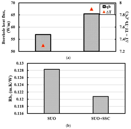
Figure 8.
Experimental results for: (a) borehole heat flux and (b) borehole thermal resistance.
The comparison between the heat fluxes and average borehole temperatures for each case could approve these results, as indicated in the following subsection.
5.1.2. Borehole Thermal Resistance
The borehole thermal resistance for each case is calculated based on Equation (7) where Tb is the average temperature of the borehole outer wall, Tf is the average fluid temperature and q’ is the average borehole heat flux per unit length. Figure 8a shows the heat flux per unit length (W/m) and the difference between the fluid temperature and borehole wall temperature for SUO and SUO + SSC cases. The heat flux is changed from 56.9 ± 1% W/m to 65.4 ± 1% W/m for SUO and SUO + SSC, respectively under the effect of ground water flow velocity of 1000 m/year, while the temperature differences are 7.3 ± 1.2% °C and 7.9 ± 1.2% °C. This indicates that the effect of groundwater flow is dominant in the SUO case. In addition, Figure 8b indicates that effect on the Rb values which decreases by 5% from 0.128 ± 1.7% m·K/W to 0.121 ± 1.7% m·K/W for SUO and SUO + SSC cases, respectively.
Moreover, the borehole temperature of the SUO is 22.5 °C, which is more than borehole temperature of SUC at 22.0 °C, means that the heat transfer rate inside the borehole for SUO is more than that in the case of SUC at which the groundwater flow cannot overcome this current. The reason for that is the supplied electrical power to the heater for SUC to maintain the fluid temperature at the predefined values is more than that of the SUO to compensate the heat energy advected by the groundwater flow. The results of SUC and SUC + SSC are not consistent. In this case, the difference between the SUC and SUO cannot be detected.
5.2. Validation of CFD Model
The temperature changes along the A-A section and B-B section in X and Y directions are used to validate the CFD simulation at a ground-water velocity of 1000 m/year for each configuration as shown in Figure 9. Figure 9 is divided into two columns, temperature variation along section A-A is shown in the left column, while temperature variation along section B-B is shown in the right column. The black scattered circles and the red triangles corresponding to the experimental and CFD results. The section A-A is extended from 0.2 m to the 0.36 m on the horizontal axis, where the water flows in the reverse direction. Section B-B is extended from 0.2 m to 0.48 m in the vertical direction. Figure 9 indicates that the soil temperature increases in the direction of groundwater flow, so the soil temperature at the upstream is lower than that at downstream of the borehole. In addition, the borehole temperature at an upstream is more than that of the downstream. More details and explanations are included in the following sections. These figures show good agreement between the CFD results and the experimental measurements with an average error value listed in Table 5.
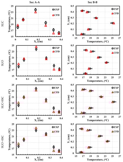
Figure 9.
CFD model validation.
Table 5.
Average error values between CFD and experimental measurements.
After validating the CFD simulation, it was used to study the impact of changing the groundwater velocity on the heat transfer inside the borehole for each case. In these simulations, the groundwater changes from 0 m/year, which corresponds to the heat transfer through saturated soil, 100 m/year, 300 m/year, 500 m/year and 1000 m/year. To conduct a fair comparison, the operating conditions are fixed in all cases as listed in Table 6.
Table 6.
Operating conditions used in these simulations.
5.3. Simulation Results
5.3.1. Borehole Temperature Contours
As mentioned in Section 5.1.2, the differences in Rb between SUC and SUO cannot be detected due to a large error of ±10 % in the measurement of the Rb. Hence, a two-dimensional CFD model is developed to predict the values of Rb in all cases under different groundwater velocities. By CFD simulation, the borehole outer wall temperature and the borehole wall heat flux are predicted, and Rb is analyzed as well.
The borehole temperature distribution contours for each case at every groundwater velocity is summarized in Figure 10. Figure 10 demonstrates the effect of increasing groundwater flow velocity on transferring the heat by advection from the center of the borehole to the outer boundary.
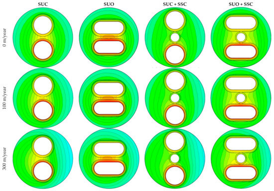
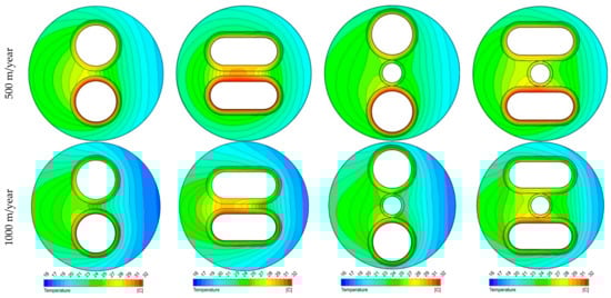
Figure 10.
Borehole temperature distribution contours for each configuration at different groundwater velocity.
For the saturated case without groundwater flow, the temperature inside the borehole is almost symmetrical around the vertical section B-B and the borehole wall temperature at Tb1 and Tb2 is 21.8 °C in SUC and SUC+SSC cases, while it is 22.6 °C in SUO and SUO + SSC cases. The heat is transferred mainly by conduction and convection through the fluid-filled bores between solid particles, therefore this result leads to that the heat transfer rate from the SUO to the borehole is more than that transferred from SUC, and it enhanced more when using the spacer.
Increasing the groundwater flow increases the temperature differences between Tb1 and Tb2, where Tb1 decreases and Tb2 increases accordingly. The maximum temperature differences occurred at 1000 m/year which reached 6.1 °C, 5.7 °C, 5.3 °C and 5.3 °C for SUC, SUO, SUC + SSC and SUO + SSC, respectively. In addition, the temperature at the center of the borehole in between the two tubes is correspondingly changed from one case to another. For SUC, it changed from 26.2 °C to 28.0 °C when groundwater velocity changed from 0 m/year to 1000 m/year. However, it changes from 29 °C to 30 °C for the SUO case. For SUC + SSC and SUO + SSC, the maximum center temperature at a velocity of 1000 m/year was 26 °C and 27.5 °C, respectively as shown in Figure 11.
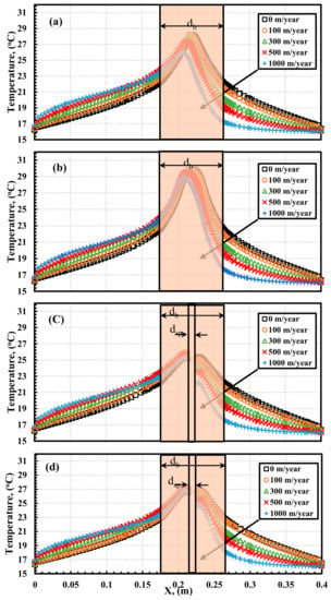
Figure 11.
Soil temperature along X-X line: (a) SUC; (b) SUO, (c) SUC + single spacer with circular cross-section (SSC) and (d) SUO + SSC.
5.3.2. Borehole Thermal Resistance (Rb)
As a result of the fluid temperature being fixed in the CFD simulation at 30.5 °C, the borehole thermal resistance (Rb) depends on both the borehole wall temperature (Tb) and the borehole wall heat flux per length (q’). Figure 12 shows the changes in Tb and q’ for each configuration at different groundwater velocities. At the same groundwater velocity, the SUO case shows higher Tb than SUC, and adding a spacer increases the Tb more.
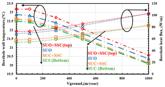
Figure 12.
Borehole heat flux and borehole wall temperature.
At saturation condition, the Tb was 22.5 °C and 23.2 °C for SUC and SUO + SSC with a difference of 0.7 °C, while increasing the groundwater velocity to 1000 m/year decreases the difference to 0.5 °C. In addition, for each case, increasing the groundwater velocity decreases the borehole water temperature due to dissipating the heat energy transferred by advection from the borehole wall in the direction of groundwater flow. Additionally, it decreases the thermal interaction between the two legs of the U-tube.
In addition, the same explanation can be used to describe the difference between q’ values of SUC and SUC + SSC. However, increasing the groundwater flow velocity increases the heat transfer rate from the borehole wall to the undisturbed soil. There is no significant impact of using a spacer in between the U-tube legs when the groundwater flow velocity increased. This is because the existence of the spacer blocked the path of groundwater between the U-tube legs. For SUO + SSC, the q’ increased from 72.5 W/m at 0 m/year to 103.0 W/m at 1000 m/year, the heat flux increased by 42.1%, while it increased by 52.3% for SUC case.
At a groundwater velocity of 1000 m/year, there is no noticeable impact of using a spacer. The oval cross-section increases the q’ by 27.3% at saturation condition and by 25.1% at the groundwater velocity of 1000 m/year.
Finally, the borehole thermal resistance (Rb) for each case at various groundwater velocities is shown in Figure 13. Under saturation condition, the Rb for SUC was 0.15 m·K/W and changed to 0.13 m·K/W with using the spacer in the SUC + SSC case. As the spacer decreases the thermal interaction between the two legs of the U-tube, it decreases the Rb by 13.3%. In addition, the Rb decreased by 9% and it changed from 0.11 m·K/W to 0.1 m·K/W with a spacer. In addition, the oval cross-section with spacer SUO + SSC decreases the Rb by 33% compared with SUC.
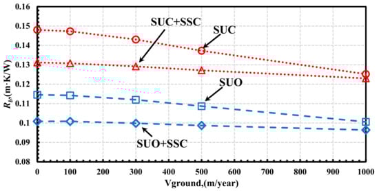
Figure 13.
Borehole thermal resistance at different groundwater flow velocities.
At the groundwater velocity of 1000 m/year, the Rb for SUC decreases to 0.12 m·K/W with a 15.5% decrement compared with saturation condition. Additionally, it decreased only by 4% for the SUO + SSC case as listed in Table 7. The impact of using a spacer decreased the Rb by only 1.5% and 4% for the SUC and SUO cases, respectively.
Table 7.
Decrement percentage in Rb when groundwater increased from 0 m/year to 1000 m/year.
6. Conclusions
The effect of groundwater flow on the thermal performance of the ground heat exchanger with a unique oval cross-section is experimentally and numerically investigated and compared with the customary circle cross-section tubes. A new small-scale laboratory experiment was built to mimick the full-scale ground heat exchanger where two separated tubes filled with water and equipped with two electrical heaters are used to replicate the U-tube heat exchanger. The two heaters keep the temperature difference between the two tubes at 3 °C using two PID controllers and temperature feedback. Four configurations are investigated; single U-tube with circular cross-section (SUC), single U-tube with an oval cross-section (SUO), single U-tube with circular cross-section and single spacer with circular cross-section (SUC + SSC) and single U-tube with an oval cross-section and single spacer with circular cross-section (SUO + SSC). The soil temperature distributions along the horizontal and vertical axis are measured and recorded simultaneously with measuring the electrical energy injected into the fluid, and the borehole wall temperature is measured as well; consequently, the borehole thermal resistance (Rb) is calculated. The experiments are carried out with a groundwater velocity of 1000 m/year. Moreover, two-dimensional and steady-state CFD simulations are developed to predict the Rb of each configuration at various groundwater flow velocities. The main conclusions are summarized as follows:
- The differences in Rb between the SUC and SUO cannot be detected experimentally due to large error of ±10% in the measurement of the Rb;
- The CFD model shows a good agreement with the experimental results with an average error value of 3%;
- For the saturated case without groundwater flow:
- i.
- The temperature inside the borehole is almost symmetrical around the vertical section because the heat is transferred mainly by conduction and convection through the fluid-filled bores between solid particles;
- ii.
- The heat transfer rate from the SUO to the borehole increased by around 15% of that transferred from SUC;
- iii.
- The Rb for SUC is decreased by 13%, it was 0.15 m·K/W and changed to 0.13 m·K/W with using spacer in the SUC + SSC case, and by 9% for SUO case, it changes from 0.11 m·K/W to 0.1 m·K/W;
- iv.
- In addition, the oval cross-section with spacer SUO + SSC decreases the Rb by 33% compared with SUC;
- At the groundwater velocity of 1000 m/year:
- i.
- The Rb for SUC decreases to 0.12 m·K/W with a 15.5% decrement compared with saturation condition, while it decreased by 4% for the SUO + SSC case;
- ii.
- in addition, using the spacer decreases the Rb by 1.5% and 4% for the SUC and SUO cases.
Accordingly, oval shape shows a better thermal performance under the impact of groundwater flow than the customary U-tube. It boosts the COP and cut down the operating cost of the GSHP systems. Therefore, the author recommends to use the U-tube with an oval cross-section in regions with a potential of fast groundwater flow. In addition, the SUO U-tube can fit easily inside the tight casing and borehole which is practically more cost-effective for construction, environmentally friendly as it saves the surrounding environment and it is preferable in a high-density population urban area.
7. Future Recommendations
As thermally proved through this work, using the oval cross-section with spacer attained the best performance compared to the conventional cylindrical cross-section. However, a cost analysis, payback period and long-term simulation for both designs are worthy to be investigated in the future.
Author Contributions
Conceptualization, A.A.S. and Y.S.; methodology, T.K.; software, A.A.S.; validation, A.R.; formal analysis, A.A.S.; investigation, A.A.S.; writing—original draft preparation, A.A.S.; writing—review and editing, A.A.S., A.R.; visualization, A.A.S.; supervision, K.N. All authors have read and agreed to the published version of the manuscript.
Funding
This research received no external funding
Acknowledgments
In this section you can acknowledge any support given which is not covered by the author contribution or funding sections. This may include administrative and technical support, or donations in kind (e.g., materials used for experiments).
Conflicts of Interest
The authors declare no conflict of interest.
References
- Self, S.J.; Reddy, B.V.; Rosen, M.A. Geothermal heat pump systems: Status review and comparison with other heating options. Appl. Energy 2013, 101, 341–348. [Google Scholar] [CrossRef]
- Sarbu, I.; Sebarchievici, C. General review of ground-source heat pump systems for heating and cooling of buildings. Energy Build. 2014, 70, 441–454. [Google Scholar] [CrossRef]
- Serageldin, A.A.; Abdelrahman, A.K.; Ookawara, S. Earth-Air Heat Exchanger thermal performance in Egyptian conditions: Experimental results, mathematical model, and Computational Fluid Dynamics simulation. Energy Convers. Manag. 2016, 122, 25–38. [Google Scholar] [CrossRef]
- Zhu, L.; Chen, S.; Yang, Y.; Sun, Y. Transient heat transfer performance of a vertical double U-tube borehole heat exchanger under different operation conditions. Renew. Energy 2019, 131, 494–505. [Google Scholar] [CrossRef]
- Nagano, K. Standard Procedure of Standard Thermal Response Test, IEA ECES, ANNEX21; IEA report; IEA: Paris, France, 2011; Volume 21. [Google Scholar]
- Han, Z.; Zhang, S.; Li, B.; Ma, C.; Liu, J.; Ma, X.; Ju, X. Study on the influence of the identification model on the accuracy of the thermal response test. Geothermics 2018, 72, 316–322. [Google Scholar] [CrossRef]
- Ma, L.; Gao, Z.; Wang, Y.; Sun, Y.; Zhao, J.; Feng, N. Numerical Simulation of Soil Thermal Response Test with Thermal-dissipation Corrected Model. Energy Procedia 2017, 143, 512–518. [Google Scholar] [CrossRef]
- Zhang, Y.; Hao, S.; Yu, Z.; Fang, J.; Zhang, J.; Yu, X. Comparison of test methods for shallow layered rock thermal conductivity between in situ distributed thermal response tests and laboratory test based on drilling in northeast China. Energy Build. 2018, 173, 634–648. [Google Scholar] [CrossRef]
- Sakata, Y.; Katsura, T.; Nagano, K. Multilayer-concept thermal response test: Measurement and analysis methodologies with a case study. Geothermics 2018, 71, 178–186. [Google Scholar] [CrossRef]
- Bandos, T.V.; Montero, A.; Fernández, E.; Santander, J.L.; Isidro, J.M.; Pérez, J.; de Córdoba, P.J.; Urchueguía, J.F. Finite line-source model for borehole heat exchangers: Effect of vertical temperature variations. Geothermics 2009, 38, 263–270. [Google Scholar] [CrossRef]
- Li, B.; Han, Z.; Hu, H.; Bai, C. Study on the effect of groundwater flow on the identification of thermal properties of soils. Renew. Energy 2018, 6–13. [Google Scholar] [CrossRef]
- Luo, J.; Tuo, J.; Huang, W.; Zhu, Y.; Jiao, Y.; Xiang, W.; Rohn, J. Influence of groundwater levels on effective thermal conductivity of the ground and heat transfer rate of borehole heat exchangers. Appl. Therm. Eng. 2018, 128, 508–516. [Google Scholar] [CrossRef]
- Samson, M.; Dallaire, J.; Gosselin, L. Influence of groundwater flow on cost minimization of ground coupled heat pump systems. Geothermics 2018, 73, 100–110. [Google Scholar] [CrossRef]
- Smith, D.C.; Elmore, A.C. The observed effects of changes in groundwater flow on a borehole heat exchanger of a large scale ground coupled heat pump system. Geothermics 2018, 74, 240–246. [Google Scholar] [CrossRef]
- Akhmetov, B.; Georgiev, A.; Popov, R.; Turtayeva, Z.; Kaltayev, A.; Ding, Y. A novel hybrid approach for in-situ determining the thermal properties of subsurface layers around borehole heat exchanger. Int. J. Heat Mass Transf. 2018, 126, 1138–1149. [Google Scholar] [CrossRef]
- Hu, J. An improved analytical model for vertical borehole ground heat exchanger with multiple-layer substrates and groundwater flow. Appl. Energy 2017, 202, 537–549. [Google Scholar] [CrossRef]
- Zhang, L.; Zhang, Q.; Huang, G.; Ma, X. Transient Ground and Grout Parameters Estimation Method for a Ground-Coupled Heat Pump System with Sandbox TRT Reference Data. Procedia Eng. 2017, 205, 2662–2669. [Google Scholar] [CrossRef]
- Choi, W.; Ooka, R. Effect of natural convection on thermal response test conducted in saturated porous formation: Comparison of gravel-backfilled and cement-grouted borehole heat exchangers. Renew. Energy 2016, 96, 891–903. [Google Scholar] [CrossRef]
- Zheng, T.; Shao, H.; Schelenz, S.; Hein, P.; Vienken, T.; Pang, Z.; Kolditz, O.; Nagel, T. Efficiency and economic analysis of utilizing latent heat from groundwater freezing in the context of borehole heat exchanger coupled ground source heat pump systems. Appl. Therm. Eng. 2016, 105, 314–326. [Google Scholar] [CrossRef]
- Coleman, T.I.; Parker, B.L.; Maldaner, C.H.; Mondanos, M.J. Groundwater flow characterization in a fractured bedrock aquifer using active DTS tests in sealed boreholes. J. Hydrol. 2015, 528, 449–462. [Google Scholar] [CrossRef]
- Li, H.; Nagano, K.; Lai, Y. A new model and solutions for a spiral heat exchanger and its experimental validation. Int. J. Heat Mass Transf. 2012, 55, 4404–4414. [Google Scholar] [CrossRef]
- Li, W.; Li, X.; Peng, Y.; Wang, Y.; Tu, J. Experimental and numerical investigations on heat transfer in stratified subsurface materials. Appl. Therm. Eng. 2018, 135, 228–237. [Google Scholar] [CrossRef]
- Wan, R.; Chen, M.; Huang, Y.; Zhou, T.; Liang, B.; Luo, H. Evaluation on the heat transfer performance of a vertical ground U-shaped tube heat exchanger buried in soil–polyacrylamide. Exp. Heat Transf. 2017, 30, 427–440. [Google Scholar] [CrossRef]
- Erol, S.; François, B. Efficiency of various grouting materials for borehole heat exchangers. Appl. Therm. Eng. 2014, 70, 788–799. [Google Scholar] [CrossRef]
- Li, H.; Nagano, K.; Lai, Y. Heat transfer of a horizontal spiral heat exchanger under groundwater advection. Int. J. Heat. Mass Transf. 2012, 55, 6819–6831. [Google Scholar] [CrossRef]
- Beier, R.A.; Smith, M.D.; Spitler, J.D. Reference data sets for vertical borehole ground heat exchanger models and thermal response test analysis. Geothermics 2011, 40, 79–85. [Google Scholar] [CrossRef]
- Li, W.; Dong, J.; Wang, Y.; Tu, J. Numerical Modeling of a Simplified Ground Heat Exchanger Coupled with Sandbox. Energy Procedia 2017, 110, 365–370. [Google Scholar] [CrossRef]
- Zhao, T.; Yu, M.; Rang, H.; Zhang, K.; Fang, Z. The influence of ground heat exchangers operation modes on the ground thermal accumulation. Procedia Eng. 2017, 205, 3909–3915. [Google Scholar] [CrossRef]
- Morrone, B.; Coppola, G.; Raucci, V. Energy and economic savings using geothermal heat pumps in different climates. Energy Convers. Manag. 2014, 88, 189–198. [Google Scholar] [CrossRef]
- Eslami-nejad, P.; Bernier, M. Freezing of geothermal borehole surroundings: A numerical and experimental assessment with applications. Appl. Energy 2012, 98, 333–345. [Google Scholar] [CrossRef]
- Lee, C.K.; Lam, H.N. A modified multi-ground-layer model for borehole ground heat exchangers with an inhomogeneous groundwater flow. Energy 2012, 47, 378–387. [Google Scholar] [CrossRef]
- Gustafsson, A.M.; Westerlund, L.; Hellström, G. CFD-modelling of natural convection in a groundwater-filled borehole heat exchanger. Appl. Therm. Eng. 2010, 30, 683–691. [Google Scholar] [CrossRef]
- Fan, R.; Jiang, Y.; Yao, Y.; Shiming, D.; Ma, Z. A study on the performance of a geothermal heat exchanger under coupled heat conduction and groundwater advection. Energy 2007, 32, 2199–2209. [Google Scholar] [CrossRef]
- Diao, N.; Li, Q.; Fang, Z. Heat transfer in ground heat exchangers with groundwater advection. Int. J. Therm. Sci. 2004, 43, 1203–1211. [Google Scholar] [CrossRef]
- Sutton, M.G.; Nutter, D.W.; Couvillion, R.J. A Ground Resistance for Vertical Bore Heat Exchangers With Groundwater Flow. J. Energy Resour. Technol. 2003, 125, 183. [Google Scholar] [CrossRef]
- Gu, Y. Effect of Backfill on the Performance of a Vertical U-tube Ground-Coupled Heat Pump. Ph.D. Thesis, Texas A&M University, College Station, TX, USA, 1995. [Google Scholar]
- Jahangir, M.H.; Sarrafha, H.; Kasaeian, A. Numerical modeling of energy transfer in underground borehole heat exchanger within unsaturated soil. Appl. Therm. Eng. 2018, 132, 697–707. [Google Scholar] [CrossRef]
- Biglarian, H.; Abbaspour, M.; Saidi, M.H. A numerical model for transient simulation of borehole heat exchangers. Renew. Energy 2017, 104, 224–237. [Google Scholar] [CrossRef]
- Serageldin, A.A.; Sakata, Y.; Katsura, T.; Nagano, K. Thermo-hydraulic performance of the U-tube borehole heat exchanger with a novel oval cross-section: Numerical approach. Energy Convers. Manag. 2018, 177, 406–415. [Google Scholar] [CrossRef]


© 2020 by the authors. Licensee MDPI, Basel, Switzerland. This article is an open access article distributed under the terms and conditions of the Creative Commons Attribution (CC BY) license (http://creativecommons.org/licenses/by/4.0/).