A Qualitative Control Approach to Reduce Energy Costs of Hybrid Energy Systems: Utilizing Energy Price and Weather Data ^†

Abstract

Nowadays, many buildings are equipped with various energy sources. The challenge is how to efficiently utilize their energy production. This includes decreasing the share and costs of external energy—usually electrical energy delivered from the grid. The following study presents a qualitative approach with a combined control to solve the problem. The approach is demonstrated using a simulated residential building equipped with a hybrid energy system: a thermal energy storage combined with an electrical heater, a geothermal heat pump and a solar thermal collector. Consequently, the share of renewable energy was increased and, conversely, costs of the external energy from grid decreased by 12.2%. The results were based on a qualitative approach and the algorithm which predicts the need of energy of the building over the next 6 h with the aid of weather forecasting. This approach included a storage tank of 300 L. The energy costs can be further decreased 7.7% by increasing thermal storage capacity and modifying the control algorithm. In all cases, the indoor conditions were kept at a comfortable level. However, if the room temperature is temporarily allowed to slightly drop a few degrees during the heating season, the energy costs were further reduced.

1. Introduction

The variety of renewable energy systems is growing rapidly. Nowadays, many buildings utilize a combination of various energy sources known as hybrid energy systems. Existing combinations of equipment and systems are multiple due to the diversity of energy sources, heating and cooling options, usage, number and type of energy storages, and control strategies [1]. In hybrid energy systems, some of the renewable energy generators behave stochastically due to the fact of their dependent nature [2]. Therefore, their performance and efficiency highly depend on weather conditions, e.g., solar radiation, wind, etc. The challenge is how to control such a combined energy system in order to take full advantage of the renewable energy sources. Hence, the controller of energy systems should aim to take full advantage of the renewable energy sources while simultaneously decreasing the share of the external energy to be purchased. The external energy is typically electrical power supplied from a grid. Power supply companies charge their consumers according to different tariff schemes, for example, dynamic electricity tariff. Typically, the price of electricity follows an hourly changing curve based on the estimated power demand of the network in the following day/hours. Thus, the customer can control energy costs using less power during daily peak times, by shifting electrical loads [3,4,5].

Numerous studies have attempted to minimize the operating cost of a hybrid energy system through a variety of methods. An early example includes smart control and building automation in residential buildings [5]. At the same time, researchers began to investigate the effect of using energy storage to minimize operating costs [6,7]. Several years later, they started to use different control approaches such as price-responsive heating system [8] and load shifting [9]. The latest papers study the impact of optimum sizing of energy systems on the energy costs [10,11]. Alimohammadisagvand et al. [12,13] studied the influence of demand response actions on electricity cost in residential buildings without sacrificing the thermal comfort. They utilized demand response control algorithms to shift electricity demand of building towards lower electricity price periods. Psimopoulos [14] developed operational control strategies for heating system of a single-family house with an exhaust air heat pump, a photovoltaic system and energy storage. His aim was to evaluate the benefit of such control strategies on energy use and economic performance.

Cost effective operation of the hybrid energy system requires simultaneous control of all the sub-systems. This is possible by using the qualitative approach consisting a qualitative model of the energy systems combined with a control algorithm. The latter is created utilizing multiple states for each energy system and sequential transitions from one state to another. Each state of the system is unique, specified by the current condition of the systems and history data of the inputs. A decision to transfer from one state to another is based on the qualitative reasoning of the heating process. The following pages show how the qualitative approach can be used to reduce the costs of external energy which consists of electricity supplied from a grid.

Due to the variety of approaches, it is not straightforward to compare the obtained results to those reported in corresponding projects [1,2,3,4,5,6,7,8,9,10,11,12,13,14]. Many of them concern cases where the building environment is limited, they focus directly on cost reduction algorithms or due to the fact of climatic reasons, the approach is technically different. The advantage of the proposed approach is to run a simulation in a realizable building environment which also considers the occupants, their living environment and domestic hot water production together with several energy systems and creates a comprehensive method to achieve notable cost reductions of electrical energy. The results cover the whole year in the climate of Southern Finland but concentrate on heating season. Similar results are not conceivable using a conventional but still typical control method which is based on independent control of each energy system.

The following results are based on a several year project. Some of the results were earlier published as a conference paper, when the research was still going on and the simulation environment including the building and energy systems was developing [15]. This article presents the revised results, analyses and discusses the subject more thoroughly on energy cost reduction of a hybrid energy system.

2. The Simulation Model, Energy Systems and Their Control

The residential building, its environmental conditions, Heating, Ventilating and Air-Conditioning (HVAC) and energy systems including their operation and inner loads were modelled in transient systems simulation Program; TRNSYS (17, The University of Wisconsin, Madison, Wisconsin, USA). The total floor area of the building is 96 m² and the volume is 408 m³, consisting of three zones in two stories. The structures, indoor climate, heating and ventilation were designed according to The National Building Code of Finland part D2 [16]. In the simulation, the air change rate for each zone was set to 0.5 L/h throughout the year, without heat recovery. The internal heat loads were scheduled according to the assumed usage of a detached house.

The building was assumed to be in Southern Finland. Therefore, weather data of the Typical Meteorological Year (TMY) from the city of Helsinki were used. Finland is one of the Nordic countries with a cold climate. Finland is divided into four climatic zones. The city of Helsinki is located in zone I, with a design temperature of −26 °C for winters.

As a result, the total heating energy demand for the space heating and for the domestic hot water was a maximum power of 7.2 kW. The simulation was performed for the entire building, but the space heating system was built only for one zone on the ground floor. Thus, the presented energy demand and the maximum power concerned only the zone. The simulation started at the beginning of the year with the time step set to one minute.

2.1. The Energy Systems

The hybrid energy system consisted of one hot water tank as energy storage and three energy sources, solar collector, geo-thermal heat pump and electrical heater. The hybrid energy systems and the transferring connections are illustrated in Figure 1. The solar collector’s circuit consisted of three 2.5 m² solar collectors, 27 W circulating pump and 30 m piping. The circulating liquid was a water–glycol mixture which was separated from the tank water with a heat exchanger. The maximum heating power of the solar collector was 5 kW.

The geo-thermal heat pump (5.9 kW) consisted of a water-to-water heat pump, load and source side circulating pumps, and a vertical U-tube heat exchanger in the ground operating as a heat source. The borehole was 175 meters deep, where a 35% ethanol–water liquid mixture was circulated in a PolyEthylene Medium (PEM) pipe. The borehole and the building were connected to horizontal pipes (20 m). The properties of the pipes were the same as those in the borehole.

A cylindrical, insulated steel tank of 300 L, installed in a vertical position, served as energy storage. The tank contained input and output connections and inner heat exchangers for domestic hot water and the solar collector. In addition, the tank was equipped with an electrical heater element (5 kW). Due to the stratified water temperature, connections were designed vertically in different elevations (Figure 1). The horizontal lines of the figure illustrate how the tank was divided into eight equal-sized nodes, starting from the uppermost node in Figure 1. For instance, the domestic hot water output was connected to Node-1, where the output water temperature was kept at 55 °C.

The floor heating consists of a pump-driven circuit supplying water of 40 °C. The maximum power of the space heating is 4 kW. The structure and sizing of the energy systems are pragmatically selected in accordance with common design practices for a single-family house.

2.2. Thermostat Controls

The storage tank, shown in Figure 1, provided heat both for the floor heating and for the domestic hot water. The set point temperature of the domestic hot water was 55 °C. This was controlled by the thermostat (1), locating in upper part of the tank (Node-1), where the outlet to the domestic hot water was located.

In the simulation, the room temperature was controlled by two thermostats (2) and (3), based on indoor air and floor surface temperatures which were set at 21.5 °C and 29 °C, respectively. If both temperatures dropped below the set points, floor heating circulating pump started. However, the space heating control was independent of the energy systems’ controls.

The heat pump and the electrical heater are connected to a two-stage thermostat (4) installed on Node-4 (Figure 1). If the Node-4 temperature drops below the setpoint, the heat pump starts. In case, if the node temperature still drops, the electrical heater also turns on. The electrical heater acts mainly as back-up energy generator providing additional heating power during the high demand periods. If the temperature of Node-1 exceeds the upper limit temperature, the heat pump turns off.

The solar collector control (not shown in Figure 1) acts like a thermostat. The circulating pump turns on if the outlet temperature of the solar collector exceeds the inlet temperature and simultaneously higher than the Node-4 temperature. The above strategy, where each energy system operates independently based only on local thermostats is later referred as a conventional approach, conventional control or conventional method. Due to the independent operation of energy systems and the lack of connection to the energy cost information, the conventional approach does not reduce the costs of the external energy supplied from the grid. Therefore, the conventional method is used in comparison with the proposed qualitative method. The comparison gives an estimate of the resulting cost reductions of the qualitative method.

2.3. The Qualitative Control Strategy

The qualitative approach, also later referred to as qualitative control or the qualitative method, aims to efficiently utilize the renewable energy sources and simultaneously, to produce domestic hot water and maintain indoor conditions comfortable. Principally, the idea is to reduce the costs caused by external electrical energy supplied from the grid. This is implemented by periodically estimating the future need of heating power and choosing the best cost-effective means to produce power. In practice, the proposed method shifts the load of electrical power when the tariff is high by using stored heating energy of the tank, and reversely, when the tariff is low, forwards heat generation to be stored in the tank. The following approach is based on time-varying electricity prices, changing dynamically once in an hour. Hourly price information is provided to the user 24 h in advance by the power supply company. Figure 2 shows the electricity price variations against hours of the year.

The main difference between the qualitative and conventional approach is that the former is a comprehensive control which supervises all energy systems simultaneously. The conventional approach means a set of independent energy systems controlled by local thermostats. However, the qualitative control takes advantage of the conventional control, i.e., both approaches use the same set points, parameters and thermostats. Thus, the qualitative control supervises and utilizes the conventional control. 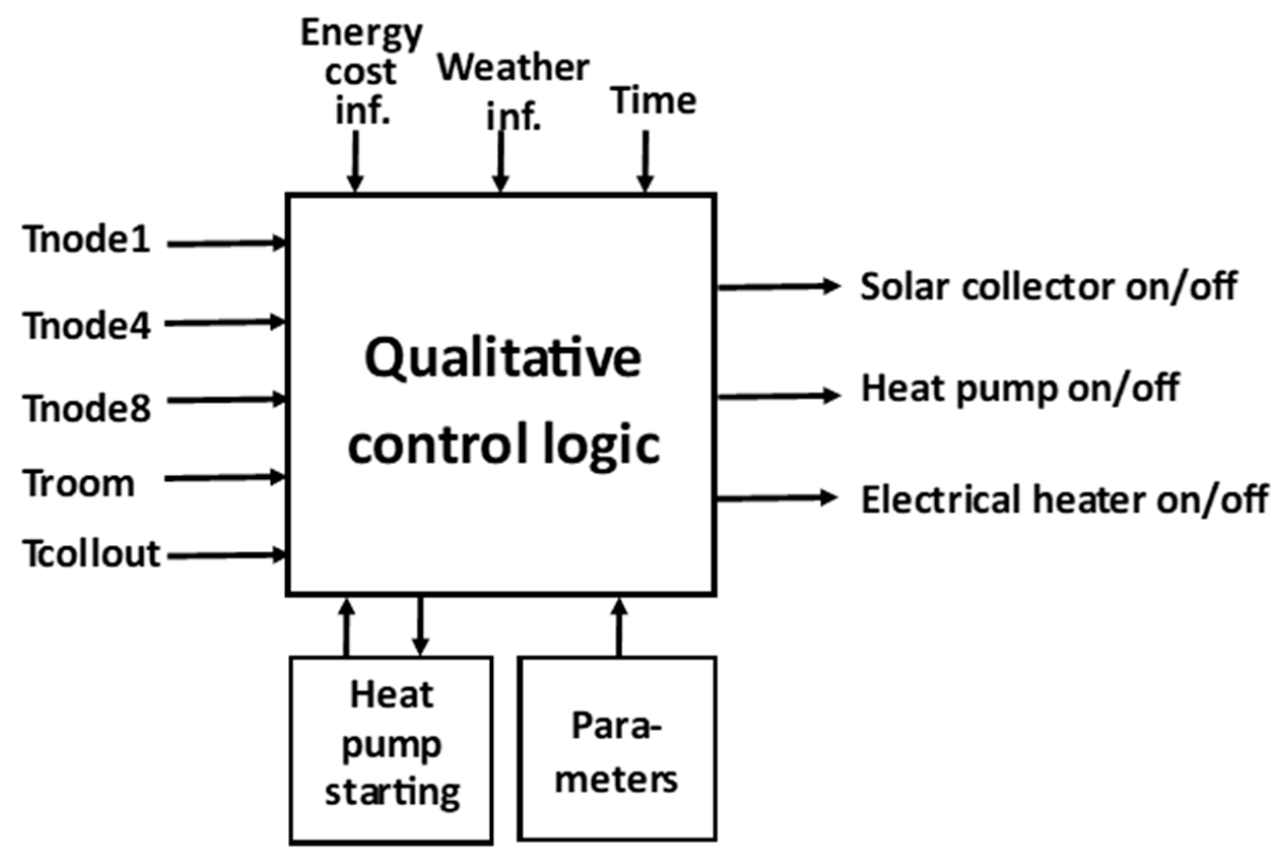Figure 3 outlines the qualitative control system which performs the designed operations when combined with the energy systems shown in Figure 1. The left side of the figure illustrates the input signals of the system, consisting of temperatures inside the tank, room and solar collector output; the upper side are time, weather and electricity hourly price inputs. The outputs are connected to the energy systems. Each output signal turns on or off the circulating pump of the solar collector or the heat pump including the compressor and its circulating pumps or the auxiliary heater.

The geothermal heat pump has a special role in the strategy. The heat pump consumes most of the electrical power supplied from the grid. Therefore, by delaying its operation, load shifting becomes effective. The starting time and length of the load shifting period depends on several variables. They are evaluated in a computer program which determines the time and length of the period and operates parallel to the control logic (Figure 3).

2.4. The Control Logic

The qualitative approach consists of the qualitative model of the energy systems combined with a control algorithm. The model was developed by analysing all different states of the energy systems. However, the idea was not to create a strict mathematical model typical in control engineering but to combine different kinds of knowledge together which enables reasoning and transitions from one state to another. Each state of the system is unique and subject to one or more conditions which are modified into inequalities and equalities. The conditions are created using time, former states, current and history data of inputs (Figure 3). Finally, a software algorithm combines all details together and implements the control.

In practice, the control logic is a collection of IF–THEN–ELSE commands, where conditions are combined with Boolean functions. Once a minute in every time step, the computer program goes through all of them. If a condition is true, the program turns on or off an energy system and/or determines the transition to the next state (Figure 4).

The above control logic can be combined with the TRNSYS simulation software either using a Fortran component compiled and integrated with the simulation software or calling an external EXCEL-program at each time step. The current version has been done using the latter method, which gives more flexibility in implementation of the logic.

2.5. Prioritizing Energy Systems

All three energy systems operate with the aid of electrical energy. A natural way to reduce external energy costs is to prioritize energy sources based on the ratio of useful heating power provided by the energy system compared to the electrical input power to that system. This is known as the coefficient of performance (COP). Among these three systems, solar collector has the highest COP. Therefore, the strategy makes the solar collector, which needs only a little quantity of electrical power to run the circulating pump, as a top priority. In principle, the solar collector feeds the tank all the time, whenever the collector output temperature is greater than the bottom and the middle node temperatures of the tank, i.e., $(T_{CollOut}>T_{Node8})\wedge (T_{CollOut}>T_{Node4})$. A necessity safety condition is that at the same the time water temperature on the top node of the tank is not too high: $(T_{Node1}<95℃)$. If the collector output temperature is high enough, but the middle node temperature rises over the limit $\left(T_{Node4}>55℃\right)$, then the tank is fully loaded. A similar decision is made if the water temperature on the top of the tank is too high $\left(T_{Node1}>95℃\right)$.

The geothermal heat pump can provide major amount of heat for the building, but it consumes a considerable portion of total electrical energy. Therefore, controlling the heat pump plays a central role in the control strategy to reduce energy costs. The operation of the geothermal heat pump depends on several conditions. First, in the beginning of the six h period, the control algorithm checks if the tank needs charging and determines the best cost-effective charging period. The same subroutine is also called if the room temperature decreases under the minimum allowable room temperature T_L, i.e., $T_{Room}<T_L$ and the same applies when the middle node temperature of the tank is decreasing, i.e., $T_{Node4}<54℃$. The minimum allowable room temperature T_L is an input parameter of the control algorithm, and usually set to 21.0 $℃$. The heat pump operates until $T_{Node4}>55℃$ after starting. If the solar collector output temperature exceeds the bottom temperature of the tank $(T_{CollOut}>T_{Node8})\wedge (T_{CollOut}>T_{Node4})$, both energy systems may operate at the same time.

The electrical heater has the lowest COP, approximately one. That is why it has the smallest priority and a minor role in heat production. Its main function is to operate as a back-up energy system to support other energy systems in producing domestic hot water and in keeping indoor conditions comfortable. The electrical heater is controlled by the thermostat (4), installed in Node-4, and its operation depends on the water temperature of $T_{Node4}$. The electrical heater may operate for longer time period in circumstances where the energy price is low.

2.6. Predicting the Need of Energy with the Aid of Weather Forecast

Estimating the need of energy for the whole building is made periodically once every six h. Six h is roughly the period a 300 L tank can provide the whole building’s energy demand in most outdoor conditions during winter. The first step is to check the current amount of heat (Q) available stored in the hot water tank.

$$Q={\mathrm{C}}_{p}m\left(T_a-T_{ma}\right)$$

(1)

where ${\mathrm{C}}_p$ refers to specific heat and m to the mass of water. $T_a$ represents the current water temperature of the tank, measured from Node 4, and $T_{ma}$ is the minimum allowable water temperature of the same node. The $T_{ma}$ is one of the parameters (Figure 3) given as an initial value of the procedure. Then, the stored amount of heat (Q) will be compared to the heating energy demand of the building with respect to the outdoor weather condition within present time up to next 6 h. The comparison gives a period of hours that the storage tank can provide heat to the floor heating and domestic water. In practice, the heating energy demand of the building will be estimated by means of a static thermal model of the building and a weather forecast.

The static thermal model is created by collecting data of a twelve-month simulation of the building. The data are further processed to a simple linear regression model which presents the heating energy demand $\dot{Q}$ of the building per one hour as a function of outdoor temperature T.

$$\dot{Q}=\dot{Q}\left(T\right)$$

(2)

It is assumed that indoor temperature is kept stable. Thus, variable T could also represent the difference between indoor and outdoor temperatures.

The next step is to check how long the storage tank can deliver domestic hot water and, at the same time, supply heat to the building through floor heating to maintain the indoor conditions at comfortable levels. This is done by testing for the largest value of M of index $i,\left(1\le i\le 6\right)$, where the following equation holds:

$$Q>{\displaystyle \sum }_{i=1}^M\dot{Q}\left(T_i\right)$$

(3)

where $T_i$ means the predicted hourly outdoor temperature, and i is 6 h forward from the current time instant. The predicted outdoor temperature is directly read from the TMY data file. In a real building, the weather forecast data would be periodically picked up from an Internet server of a weather service provider.

If M = 6, there is energy enough for the whole period and the next checking will be done again after six h. If M < 6, the heat amount of the storage tank must be increased within the next M hours. This is done by starting the geothermal heat pump. A necessity is that, at the same time, the cost of the electrical energy is low enough. If the heat pump operates for two hours, it is enough to charge the tank for the next six hours. Therefore, the control procedure tries to find a 2 h period within the next M hours, where the cost of electrical energy is lower than average. The idea is to avoid peak load times and find the maximum cost difference $C_D$ between average energy costs during continuous pair of hours i, and i + 1, i.e., $(C_i+C_{i+1})/2$ and the average energy costs $C_a$. Thus, $C_D$ can be written as:

$$C_D=max\left[\frac{(C_i+C_{i+1})}{2}-C_a\right]$$

(4)

where:

$$C_a=\frac{1}{M}{{\displaystyle \sum }}_1^M{C}_i$$

(5)

The continuous pair of hours means, the sequential hours as: $\left(i,i+1\right)\in \left\{\left(1,2\right),\left(2,3\right),\dots ,\left(M-2,M-1\right)\right\}$. If such a pair $\left(i,i+1\right)$ is found, the program starts the geothermal heat pump in the beginning of the hour i. If no such period is found, the heat pump will be started within the next hour despite the energy costs. The whole procedure is repeated after six hours.

Tabulated data are defined according to the thermal model of the building to evaluate the heating demand for the next 1 hour up to the next 6 h for the control algorithm. As shown in

Table 1. Thermal model of the building.

Outdoor Temperature Index	Q Demand for the Next 1 h (kWh)	Q Demand for the Next 2 h (kWh)	Q Demand for the Next 3 h (kWh)	Q Demand for the Next 4 h (kWh)	Q Demand for the Next 5 h (kWh)	Q Demand for the Next 6 h (kWh)
1	1.180	2.360	3.540	4.720	5.900	7.080
2	1.105	2.210	3.315	4.420	5.525	6.630
3	0.983	1.966	2.949	3.932	4.915	5.898
4	0.863	1.727	2.590	3.454	4.317	5.180
5	0.745	1.490	2.234	2.979	3.724	4.469
6	0.631	1.261	1.892	2.522	3.153	3.784
7	0.503	1.005	1.508	2.011	2.513	3.016
8	0.365	0.731	1.096	1.462	1.827	2.193
9	0.217	0.435	0.652	0.870	1.087	1.304
10	0.014	0.029	0.043	0.058	0.072	0.087

, values are based on an outdoor temperature index. The index is defined as one if the outdoor temperature is less than −25 °C $\left(T<-25°\mathrm{C}=>\mathrm{I}=1\right)$, and it is two when the outdoor temperature is within −25 °C, up to −20 °C, $\left(-25°\mathrm{C}\le T<-20°\mathrm{C}=>I=2\right)$ etc.

The above procedure assumes that the price reading period is fixed to six hours. The next step is to find out what is the effect of enlarging the period according to the size of the water tank. Therefore, the algorithm was modified, and the price reading period was extended to 10 h and the table is accordingly continued for evaluating the heating demands of up to 10 h.

3. Results, Analysis and Discussion

3.1. Test Run Arrangements

The test runs consisted of simulations of twelve months, starting at the beginning of January. The sampling time was one minute. Both methods were simulated using the same weather data, inner loads, usage and operation of the building. In both cases a 24 h day-ahead hourly tariff scheme was applied for calculating the energy costs.

We first simulated the building using the qualitative control approach. Then, the results were compared with that of a conventional method. The conventional control was put into operation simply by disconnecting the qualitative control logic. Set points and parameter values did not need to be changed after disconnection. Then, each energy system operated independently by means of the local thermostats (Figure 1). If the temperature dropped below the set point, that system turned on regardless of electricity prices and other systems operations.

The total electrical power supplied from the grid consisted of the electricity delivered to the heat pump $E_{HP}\left(h\right)$, solar thermal collector $E_{SC}\left(h\right)$ and the electrical heater $E_{AH}\left(h\right)$. Thus, the total yearly electricity costs of the systems were summed up over 8760 h of the year:

$$C_A={{\displaystyle \sum }}_{h=1}^{8760}\left\{E_{HP}\left(h\right)+E_{SC}\left(h\right)+E_{AH}\left(h\right)\right\}\times T\left(h\right)$$

(6)

where T(h) is the electricity tariff at hour h. The tariff is a 24 h-ahead hourly electricity price.

3.2. Case 1. Comparison Using a 300 L Tank and a Room Temperature Set Point at 21.5 °C

The simulation results showed that the sum of thermal energy supplied to the tank by the energy systems were 5824.7 kWh/a in the conventional method and 5798.9 kWh/a in the qualitative method. The thermal energy supplied into the tank was delivered to the building to provide thermal energy for floor heating and domestic hot water. The heat pump COP was 2.86 on average, both in the qualitative and conventional control approaches. The quantity of thermal energy generated and delivered to the building had negligible differences. A small difference in the energy consumption was found in domestic hot water production, i.e., consumption of the conventional method was higher. This was due to the slightly higher hot water temperature of the conventional method, as shown is later figure. As a conclusion, we can assume that the same amount of energy was delivered to the building by each method. Therefore, the comparison is logically valid.

The energy consumption portion of each energy system is illustrated in Figure 5.

The share of each energy system varies according to the electricity price. However, the share of heating energy production is quite different. solar collector 21%, heat pump 77%, and electrical heater 2%. Thus, solar collector, which consumes only about 2% of the electricity, produces 21% of the heating energy. The share of heating energy production is almost similar for both methods.

The results showed that the room temperature is fluctuating around the set point temperature. However, temperature variations of the two methods slightly differ from each other. Again, with the intention of reasonably comparing the room temperature stability of the methods, we defined an “‘hour-degree”—a characteristic quantity—which describes the sum of the room temperature deviations from the minimum allowable room temperature $T_L=21.0°\mathrm{C}$, measured at each time step (1/60 hour). Only room temperatures smaller than $T_L$ are included. The value of the quantity for the qualitative method was 27.9, and for the conventional method it was 38.7. The time period in which room temperature falls below 21.0 °C was 2% of the whole heating season for the qualitative and 2.8% for the conventional method. Thus, the qualitative method keeps the room temperature more stable. Figure 6 presents an example of the room temperature deviations for a short time period.

Next, the energy consumption of the two methods was compared using duration curves for both the room temperature as well as domestic hot water. The results are shown in Figure 7.

Figure 7 shows that room temperature conditions are almost similar in both methods. The domestic hot water was kept at 55 °C during 97% of the usage times in both methods. Throughout, 3% of the time, domestic hot water temperature dropped a little under 55 °C for both methods. Performance of the conventional method was slightly better. All the results above demonstrated that approximately equal quantities of energy were delivered to the building by each method; therefore, we can subsequently compare their electricity costs.

The total yearly electricity costs of the building model and energy systems controlled by the qualitative method versus the conventional method are compared in

Table 2. Comparison of electricity consumption between the conventional and Qualitative method.

Month	Electricity Costs (€)		Cost Reduction (%)
	Conventional Method	Qualitative Method
January	66.2	61.2	7.5%
February	69	64.8	6.1%
March	34.8	31.5	9.6%
April	18.9	15.4	18.7%
May	13.7	9.1	33.5%
June	12.9	6.3	51.1%
July	5.2	3.4	34.2%
August	16.1	13.8	14.1%
September	22.4	18.1	19.4%
October	28	23.8	15.0%
November	50.4	46.3	8.1%
December	50.8	47.3	6.8%
Total	388.4	341.0	12.2%

.

The revised results showed that the energy costs of the qualitative method were reduced approximately 12% compared to the conventionally controlled method. This cost reduction is consistent with the results published by Corradi et al. [8] and Nyeng, et al. [15]. In addition, the demand response control algorithm [12,13] gives also corresponding results, as well as the cost-conscious method introduced by the authors [17,18] in an earlier published article and conference paper.

Figure 8 illustrates an essential difference in the operation of the methods and how this feature affects electricity costs. The figure shows the variations of the electricity price and the on/off control signal of the geo-thermal heat pump. The conventional method turns the heat pump on and off regardless of the electricity price, but the qualitative approach avoids operation during high electricity prices. Therefore, the cumulative electricity costs of the qualitative method will be lower.

3.3. Case 2: Impact of the Tank Size on Energy Cost Reduction

The earlier results considered only one tank size and a fixed price reading period. Therefore, the second step is to determine the impact of the thermal capacity (tank size) on the total cost reduction. The same building model, energy systems and control method were applied. The only difference was that the tank size was altered from 300 L to 500 L, 750 L and finally to 1000 L. Only the qualitative method was used in this comparison. First, the price information of the next 6 h was applied. Then, the last simulation considered the case of a 1000L tank size and the price information of next 10 h in the algorithm. The simulation results of overall yearly energy costs are presented in

Table 3. Yearly energy costs for various tank sizes €/a.

Month	Tank Size (Litre)
	300	500	750	1000	1000
	Algorithm Is Based on Price Reading of Next 6 h				Based on Price Reading of Next 10 h
January	61.2	61.5	64.0	59.2	55.3
February	64.8	60.2	58.8	59.4	51.6
March	31.5	32.2	31.2	31.3	27.6
April	15.4	17.2	16.7	16.3	15.7
May	9.1	11.9	12.5	11.4	10.9
June	6.3	8.5	8.5	8.9	8.8
July	3.4	4.5	4.3	4.0	4.1
August	13.8	15.4	16.8	15.2	15.4
September	18.1	18.9	19.4	19.3	18.2
October	23.8	24.9	25.6	25.5	23.0
November	46.3	46.1	48.3	46.2	40.9
December	47.3	46.9	44.4	44.6	43.1
SUM (€)	341.0	348.3	350.4	341.2	314.7
Additional cost Reduction (%)	0.0%	−2.1%	−2.7%	−0.1%	+7.7%

. The last column contains the results of the 1000 L tank size for a 10 h price reading period.

According to the results presented in Table 3, the total yearly energy costs were either slightly increased or remained nearly the same by increasing the tank size, if the 6 h price reading period was used. It seems that the 6 h price reading period would be more suitable for the 300 L tank size, considering also the lower primary investment costs. But the combination of a 1000 L tank size and the reading period of price information for 10 h gives a further reduction of energy costs up to 7.7%. If this result is compared to the total yearly energy costs of the conventional method, the cost reduction would be 19%. The curves in Figure 9 illustrates the running costs of all alternative tank sizes controlled with the qualitative method compared to each other and to the conventional control method.

3.4. Case 3: Impact of Lower Room Temperature on Energy Cost Reduction

The third step is to study the impact of lower room temperature alternatives on total energy costs. This is useful for cases where the occupant is not at home or he/she accepts that the room temperature can be slightly dropped for a short time period. If the room temperature temporarily drops within acceptable limits, it has a direct effect on the energy consumption. Another consequence is that the control algorithm can delay the start of the geo-thermal heat pump which has a direct positive effect on energy cost reduction. Therefore, the model with a 300L tank size and qualitative control was applied, while the room temperature was allowed temporarily to drop from the set point temperature 21.5 °C to 20 °C, 19 °C and 18 °C. The model with the alternatives was simulated only for the heating season as explained later. The simulation results for the energy costs are presented in

Table 4. Yearly energy cost reduction while reducing room temperatures €/a.

Month	Energy Costs €/a
	300 Litre Tank Size
	Room Temperatures
	21.5 °C	20 °C	19 °C	18 °C
January	61.23	55.95	49.16	47.44
February	64.79	52.73	48.37	47.03
March	31.46	27.11	26.72	23.9
November	46.31	44.86	37.78	33.64
December	47.33	41.8	37.6	35.6
SUM	251.12	222.45	199.63	187.61
Cost reduction %		11.42%	20.50%	25.29%

. The results show that an additional energy costs reduction is possible to achieve, starting from 11 up to 25, depending on how many degrees the room temperature is allowed to drop. The first two degrees lower energy costs approximately 10 percent. Then, for the next two degrees, it reduces costs further 5%–7%.

Figure 10 shows how the indoor and outdoor temperatures vary during the heating season. As before, the period is limited to the heating season, because the simulated building does not provide any cooling energy during summer. This is typical in Finland, where heating dominates the total energy consumption of a residential building. Typically, cooling is not necessary in summer. Therefore, the indoor air temperature cannot be kept at comfortable levels in warm season. As shown in Figure 6 and Figure 10, the range of indoor temperature fluctuations was limited to ±2 degrees around the set point temperature. The room temperature set point alternatives (20 °C, 19 °C, 18 °C) behaved similarly except that the average temperature level was lower.

One concern of the qualitative approach comes out if the weather forecast turns out to be inaccurate or if the thermal model of the building is unsatisfactory. If outdoor temperature drops lower than predicted, the heat stored in the tank may not cover the total heating energy demand. A similar situation may happen if the thermal model of the building proposes too low energy demand for the next few hours. In both cases, the shortage of heating energy could be later appear as dropping of the indoor temperature. However, the control logic starts the heat pump immediately, when the indoor temperature drops under the prescribed minimum, and at the same time water temperature in the middle of the tank is low. Thus, except for short periods of time the indoor conditions can be kept comfortable.

In the case that the outdoor temperature is higher than predicted or the energy demand presented by the thermal model is too high, the system may operate inefficiently; cost reduction may be lower than the potential. In a real building, the weather forecast is provided by a weather service company. Thus, one possibility to address the problem is to focus on developing a more comprehensive thermal model of the building.

In order to further develop the method, one option is to apply a changing varying price reading discharge period for the tank. In the above discussion method the maximum discharge period was fixed, set to six hours for the 300 L or 10 h for 1000 L tank size. This is roughly the period the storage tank can provide the whole building energy demand in most outdoor conditions during winter. When conditions are milder, the maximum price reading period could be longer. This gives more time to find low tariff periods for operating the heat pump, resulting in more opportunities for reduction of the electricity costs.

Another option is to apply variable set point temperatures in the control algorithm instead of using thermostats with fixed set point temperatures in order to make the tank capable of storing larger quantities of energy, mainly during the lower electricity tariff periods [17]. The current method uses constant set point temperatures.

4. Conclusions

A qualitative approach was presented which aims to decrease electrical energy costs in a simulated residential building, equipped with a hybrid energy system including a geothermal heat pump and a solar thermal collector connected to a thermal energy storage with a built-in electrical heater. The qualitative method successfully dropped energy costs approximately 12 percent. At the same time, domestic hot water was sufficiently provided, and indoor air conditions were maintained at comfortable levels. The results were based on common sizing of the energy systems, typical for Southern Finland’s climate. Further increasing the tank size did not directly cause an additional decrease in the energy costs. However, increasing both the tank size and the price reading period has positive effect on the cost reduction, so that additional 7.7 percent is possible to attain. Moreover, if temporary dropping of the room temperature is accepted, the energy costs can be lowered even more. The test runs show that similar results are not conceivable using a conventional method which is based on independent control of each energy system. The proposed approach is applicable to be used in buildings located in geographical areas where the role of heating in total energy consumption is significant and all the presented energy systems become profitable to use.

References

1. Zhai, X.; Qu, M.; Yu, X.; Yang, Y.; Wang, R. A review for the applications and integrated approaches of ground-coupled heat pump systems. Renew. Sustain. Energy Rev. 2011, 15, 3133–3140. [Google Scholar] [CrossRef]
2. Su, W.; Wang, J.; Roh, J. Stochastic Energy Scheduling in Microgrids with Intermittent Renewable Energy Resources. IEEE Trans. Smart Grid 2013, 5, 1876–1883. [Google Scholar] [CrossRef]
3. Sharma, I.; Bhattacharya, K.; Canizares, C. Smart Distribution System Operations with Price-Responsive and Controllable Loads. IEEE Trans. Smart Grid 2014, 6, 795–807. [Google Scholar] [CrossRef]
4. Steen, D.; Tuan, L.A.; Carlson, O. Effects of Network Tariffs on Residential Distribution Systems and Price-Responsive Customers Under Hourly Electricity Pricing. IEEE Trans. Smart Grid 2015, 7, 617–626. [Google Scholar] [CrossRef]
5. Oldewurtel, F.; Ulbig, A.; Parisio, A.; Andersson, G.; Morari, M. Reducing peak electricity demand in building climate control using real-time pricing and model predictive control. In Proceedings of the 49th IEEE Conference on Decision and Control (CDC), Atlanta, GA, USA, 15–17 December 2010; pp. 1927–1932. [Google Scholar]
6. Kaplani, E.; Ntafogiannis, P.; Pappas, K.; Diamantopoulos, N. Dynamic load management and optimum sizing of stand-alone hybrid PV/wind system. In AIP Conference Proceedings; AIP Publishing: Melville, NY, USA, 2015; p. 150003. [Google Scholar]
7. Oldewurtel, F.; Ulbig, A.; Morari, M.; Andersson, G. Building control and storage management with dynamic tariffs for shaping demand response. In Proceedings of the 2011 2nd IEEE PES International Conference and Exhibition on Innovative Smart Grid Technologies, Manchester, UK, 5–7 December 2011; pp. 1–8. [Google Scholar]
8. Corradi, O.; Ochsenfeld, H.; Madsen, H.; Pinson, P. Controlling Electricity Consumption by Forecasting its Response to Varying Prices. IEEE Trans. Power Syst. 2012, 28, 421–429. [Google Scholar] [CrossRef] [Green Version]
9. Arteconi, A.; Hewitt, N.; Polonara, F. Domestic demand-side management (DSM): Role of heat pumps and thermal energy storage (TES) systems. Appl. Therm. Eng. 2013, 51, 155–165. [Google Scholar] [CrossRef]
10. Parvizimosaed, M.; Farmani, F.; Anvari-Moghaddam, A. Optimal energy management of a micro-grid with renewable energy resources and demand response. J. Renew. Sustain. Energy 2013, 5, 53148. [Google Scholar] [CrossRef] [Green Version]
11. Eltamaly, A.M.; Al-Shamma’A, A.A. Optimal configuration for isolated hybrid renewable energy systems. J. Renew. Sustain. Energy 2016, 8, 45502. [Google Scholar] [CrossRef]
12. Alimohammadisagvand, B.; Jokisalo, J.; Sirén, K. The potential of predictive control in minimizing the electricity cost in a heat-pump heated residential house. In Proceedings of the 3rd IBPSA-England Conference BSO, Newcastle, UK, 12–14 September 2016. [Google Scholar]
13. Alimohammadisagvand, B. Influence of Demand Response Actions on Thermal Comfort and Electricity Cost for Residential Houses. Ph.D. Thesis, Aalto University, Dipoli, Finland, 2018. [Google Scholar]
14. Psimopoulos, E. Smart Control of PV and Exhaust Air Heat Pump Systems in Single-Family Buildings. Ph.D. Thesis, Uppsala University, Uppsala, Sweden, 2019. [Google Scholar]
15. Nyeng, P.; Ostergaard, J. Information and Communications Systems for Control-by-Price of Distributed Energy Resources and Flexible Demand. IEEE Trans. Smart Grid 2011, 2, 334–341. [Google Scholar] [CrossRef] [Green Version]
16. Kalliomäki, P. Indoor Climate and Ventilation of Buildings Regulations and Guidelines 2012; European Parliament and Council Directive: Helsinki, Finland, 2012; pp. 1–42. [Google Scholar]
17. Taebnia, M.; Pakanen, J. Qualitative cost-conscious control of combined energy sources in a residential building. J. Renew. Sustain. Energy 2018, 10, 024102. [Google Scholar] [CrossRef]
18. Taebnia, M.; Heikkilä, M.; Mäkinen, J.; Kiukkonen-Kivioja, J.; Pakanen, J. Demonstrating a Qualitative Control of a Hybrid Energy System in Reducing Energy Costs of a Residential Building. In Proceedings of the IBPSA-England Conference on Building Simulation and Optimization, Cambridge, UK, 11–12 September 2018. [Google Scholar]
Figure 1. The scheme of the combined energy systems.
Energies 13 01401 g001
Figure 2. Hourly electricity price variations.
Energies 13 01401 g002
Figure 3. The proposed qualitative control of the energy systems.
Energies 13 01401 g003
Figure 4. Algorithm of the state N.
Energies 13 01401 g004
Figure 5. Electricity consumption share of energy systems: (a) conventional, (b) qualitative methods.
Energies 13 01401 g005
Figure 6. Room temperature deviations from set point temperature.
Energies 13 01401 g006
Figure 7. Duration curves: (a) room temperature, (b) domestic hot water.
Energies 13 01401 g007aEnergies 13 01401 g007b
Figure 8. The differences between the heat pump control: (a) conventional, (b) qualitative method.
Energies 13 01401 g008
Figure 9. Yearly energy costs using various tank sizes €/a.
Energies 13 01401 g009
Figure 10. Indoor and outdoor temperatures during the heating season.
Energies 13 01401 g010