A New Network for Particle Filtering of Multivariable Nonlinear Objects ^† †

Abstract

In this paper, a new object in the form of a theoretical network is presented, which is useful as a benchmark for particle filtering algorithms designed for multivariable nonlinear systems (potentially linear, nonlinear, and even semi-Markovian jump system). The main goal of the paper is to propose an object that potentially can have similar to the power system grid properties, but with the number of state variables reduced twice (only one state variable for each node, while there are two in the case of power systems). Transition and measurement functions are proposed in the paper, and two types of transition functions are considered: dependent on one or many state variables. In addition, 10 types of measurements are proposed both for branch and nodal cases. The experiments are performed for 14 different, four-dimensional systems. Plants are both linear and highly nonlinear. The results include information about the state estimation quality (based on the mean squared error indicator) and the values of the effective sample size. It is observed how the higher effective sample size resulted in the better estimation quality in subsequent cases. It is also concluded that the very low number of significant particles is the main problem in particle filtering of multivariable systems, and this should be countered. A few potential solutions for the latter are also presented.

1. Introduction

The particle filter (PF) is potentially a very good estimation method because it is based on the optimal solution resulting from Bayesian filtering rules. On the contrary, the biggest disadvantage of PFs is their need for computational power as the number of calculations grows exponentially with the number of system variables [1]. This is the reason why PF methods are usually used only for state estimation with plants of small order.

Some solutions to this problem are hybrid filters, e.g., Rao-Blackwellized PF (RBPF) [2,3] or marginalized PF [4], in which state variables are divided into two groups (one group is estimated using the PF method and the second group using Kalman Filter (KF) methods (linear, extended or unscented)).

Another solution was proposed in [5], where all state variables were divided into groups in which estimation processes were performed; however, the disadvantage of this method was a loss of information contained in measurements, which were based on state variables from two or more groups.

The Dispersed Particle Filter (DPF) was proposed by the authors in one of the previous works [6]; this method assumed that dependencies between state variables and measurements were relatively sparse (transition and measurement functions depended on a relatively small number of different state variables). These research works were performed with the power system grid as an object. Unfortunately, the number of state variables was twice higher than the number of its nodes. Therefore, the performed calculations lasted relatively long, even for small systems.

The Power System State Estimation (PSSE) issue dates back to the 1970s, when Fred Schweppe in his three papers [7,8,9] proposed the PSSE approach using the Weighted Least Squares (WLS) method. This static estimation algorithm is still used in many applications, even after fifty years.

The literature about the PSSE topic is very rich. One can find studies relying not only on the WLS algorithm, but also Kalman filters (extended EKF [10] and unscented UKF [11]), as well as artificial neural networks [12,13]. In [14], the Mixed Kalman Particle Filter (MKPF) method was proposed, which combined elements of the EKF, UKF, and PF algorithms.

Regardless of the estimation method used, a frequent solution is a division of the whole power system grid into subareas [15,16,17,18]. A similar solution was proposed by the authors for the DPF algorithm [6], where the number of subareas was equal to the node number. However, the studies were problematic due to the calculation time. Based on studies from [19], the reasonable number of particles should be about:

$$N_p=4^{N_x},$$

(1)

where $N_p$ is the particle number and $N_x$ is the number of state variables.

The main purpose of the current article is to propose a new network-type system with the number of state variables equal to the number of nodes. Thanks to this, it will be possible to conduct studies even on quite large plants in a relatively short time. The final task will be to propose a particle filter method that will operate satisfactorily (in terms of calculation time and estimation quality) even with large networks. Based on the proposed plant, the subsequent algorithm propositions will be able to be checked quickly, and calculations in power system grids will be performed for results’ confirmation only.

However, the proposed network is much more general. It enables fast preparation of even very complex objects. Hence, it can also be used by researchers who are mainly interested in nonlinear estimation issues. Therefore, we provide a very elaborate description of the proposed system in the next section. There are many specification possibilities for both transition and measurement functions. It is also planned to share the source code, which may be used to perform calculations for a given network, without the need for code modification.

In the second section, one can find the description of the particle filter algorithm and the presentation of the proposed network. The simulations performed to evaluate the approach and the results are shown in the third section. The last section contains the conclusions and future plans in this research direction.

This paper is a greatly extended version of the article presented during the 13th Federated Conference on Computer Science and Information Systems (FedCSIS 2018) [20].

For a better understanding of the content presented herein, the authors describe the most important symbols in Table 1.

Table 1. Explanations of the most important symbols used in the article.

Symbol	Explanation
$\alpha$$\beta$$\phi$n$p_J$	parameters in transition functions
$\alpha$$\gamma$$\lambda$	parameters in measurement functions
$f{l}_{i,j}^{\left(k\right)}$	line function from the $i\mathrm{th}$ to $j\mathrm{th}$ nodes
M	simulation length (number of time steps)
$m_{i,j}$${\mu }_{i,j}$	parameters of a branch
$N_{eff}$	effective sample size (number of significant particles)
$n_o^{\left(k\right)}$	noise of the $o\mathrm{th}$ measurement at the $k\mathrm{th}$ time step
$N_p$	number of particles
$N_x$	number of state variables in a plant
$P_i^{\left(k\right)}$$Q_i^{\left(k\right)}$$R_i^{\left(k\right)}$$S_i^{\left(k\right)}$$T_i^{\left(k\right)}$	nodal measurements in the $i\mathrm{th}$ node
$P_{i,j}^{\left(k\right)}$$Q_{i,j}^{\left(k\right)}$$R_{i,j}^{\left(k\right)}$$S_{i,j}^{\left(k\right)}$$T_{i,j}^{\left(k\right)}$	branch measurements between the $i\mathrm{th}$ and $j\mathrm{th}$ nodes, placed near the $i\mathrm{th}$ node
$q^{i,\left(k\right)}$	normalized weight of the $i\mathrm{th}$ particle at the $k\mathrm{th}$ time step
$v_j^{\left(k\right)}$	internal noise of the $j\mathrm{th}$ state variable
${\mathbf{x}}^{i,\left(k\right)}$	state vector of the $i\mathrm{th}$ particle at the $k\mathrm{th}$ time step
$x_j^{\left(k\right)}$	$j\mathrm{th}$ state variable at the $k\mathrm{th}$ time step
$x_j^{\left(k\right)+}$	true value of the $j\mathrm{th}$ state variable at the $k\mathrm{th}$ time step
${\hat{x}}_j^{\left(k\right)}$	estimated value of the $j\mathrm{th}$ state variable at the $k\mathrm{th}$ time step
$z_o^{\left(k\right)}$	$o\mathrm{th}$ measurement at the $k\mathrm{th}$ time step
${\mathbf{Z}}^{\left(k\right)}$	set of all measurement vectors, from the first to the $k\mathrm{th}$ time step

2. Materials and Methods

2.1. Particle Filter

A plant can be expressed by the following state-space equations:

$$\left\{\begin{array}{l}{\mathbf{x}}^{(k+1)}=\mathbf{f}\left({\mathbf{x}}^{\left(k\right)},{\mathbf{u}}^{\left(k\right)},k\right)+{\mathbf{v}}^{\left(k\right)}\hfill \\ {\mathbf{z}}^{\left(k\right)}=\mathbf{h}\left({\mathbf{x}}^{\left(k\right)},{\mathbf{u}}^{\left(k\right)},k\right)+{\mathbf{n}}^{\left(k\right)}\hfill \end{array}\right.$$

(2)

where ${\mathbf{x}}^{\left(k\right)}$ is a state vector, ${\mathbf{u}}^{\left(k\right)}$ is an input vector, ${\mathbf{z}}^{\left(k\right)}$ is an output vector, and vectors ${\mathbf{v}}^{\left(k\right)}$ and ${\mathbf{n}}^{\left(k\right)}$ are internal and measurement noises, respectively; all at the $k\mathrm{th}$ time step. The main task of the considered particle filter is to estimate the state vector $\mathbf{x}$ (2) based on the measurements and input signals.

The particle filters’ operation principle is based on recursive Bayesian filtering [21]:

$$\stackrel{\mathrm{posterior}}{\overbrace{p\left({\mathbf{x}}^{\left(k\right)}|{\mathbf{Z}}^{\left(k\right)}\right)}}=\frac{\stackrel{\mathrm{likelihood}}{\overbrace{p\left({\mathbf{z}}^{\left(k\right)}|{\mathbf{x}}^{\left(k\right)}\right)}}·\stackrel{\mathrm{prior}}{\overbrace{p\left({\mathbf{x}}^{\left(k\right)}|{\mathbf{Z}}^{(k-1)}\right)}}}{\underset{\mathrm{evidence}}{\underbrace{p\left({\mathbf{z}}^{\left(k\right)}|{\mathbf{Z}}^{(k-1)}\right)}}},$$

(3)

where ${\mathbf{Z}}^{\left(k\right)}$ is a set of measurement vectors from the first to the $k\mathrm{th}$ time step, $p\left({\mathbf{x}}^{\left(k\right)}\right|{\mathbf{Z}}^{\left(k\right)})$ is a posterior Probability Density Function (PDF), $p\left({\mathbf{x}}^{\left(k\right)}\right|{\mathbf{Z}}^{(k-1)})$ is a prior PDF, $p\left({\mathbf{z}}^{\left(k\right)}\right|{\mathbf{x}}^{\left(k\right)})$ is a likelihood, and $p\left({\mathbf{z}}^{\left(k\right)}\right|{\mathbf{Z}}^{(k-1)})$ is evidence (normalization factor).

The key idea in the considered PF is to implement the posterior PDF as a set of particles. The $i\mathrm{th}$ particle is represented by a pair $\left\{{\mathbf{x}}^{i,\left(k\right)},q^{i,\left(k\right)}\right\}$ composed of the state value and the weight. The higher the weight, the higher the probability that the value ${\mathbf{x}}^{i,\left(k\right)}$ is close to the real state vector. If the number of particles, $N_p$, is high enough, the information about the posterior PDF contained in the particle set is the same as in the continuous PDF function.

The first particle filter was proposed in 1993 by Gordon, Salmond, and Smith [22] and was called the bootstrap filter. The operation principle of this PF is presented in Algorithm 1.

Algorithm 1: bootstrap filter

Initialization: draw $N_p$ initial values ${\mathbf{x}}^{i,\left(0\right)}$ from initial PDF $p\left({\mathbf{x}}^{\left(0\right)}\right)$; set time step k = 1; Prediction: draw $N_p$ new particles from the transition model ${\mathbf{x}}^{i,\left(k\right)}\sim p\left({\mathbf{x}}^{\left(k\right)}\right|{\mathbf{x}}^{i,(k-1)})$; Update: compute the particles weights based on the measurement model ${\widehat{q}}^{i,\left(k\right)}=p\left({\mathbf{z}}^{\left(k\right)}\right|{\mathbf{x}}^{i,\left(k\right)})$; Normalization: normalize weights so that their sum is equal to 1: $$q^{i,\left(k\right)}=\frac{{\widehat{q}}^{i,\left(k\right)}}{{\sum }_{j=1}^{N_p}{\widehat{q}}^{j,\left(k\right)}},$$ where ${\widehat{q}}^{\left(k\right)}$ are unnormalized weights, calculated in Step 3. Resampling: draw $N_p$ new particles using the posterior PDF obtained in previous steps (the chance that the particle will be drawn is equal to the normalized weight); End of iteration: calculate the estimated state vector; increase the time step $k=k+1$; go to Step 2.

The considered PF can be used for both non-Gaussian distributions and complex transition models. An example of such a complex system model can be a semi-Markovian jump system [23], in which the whole system model can switch to a different structure (with some probability) described by other equations and also can go back to the previous “system equations”.

Resampling

Resampling is a very important step of the algorithm. Its main task is to prevent particles from degeneration. The Sequential Importance Sampling (SIS) is an example of the algorithm without resampling and is a direct predecessor of the PF. The above-mentioned problem relates to the effect when all but one particles have their weights equal to or near zero (and the weight of that one particle tends to 1).

The particle filter is inherently connected to resampling; hence, the first usage of resampling was presented in the same article in which the particle filter was proposed [22]. During the resampling stage, $N_p$ particles must be drawn from the PDF obtained in previous steps. At every draw stage, the probability that the specific particle will be drawn is equal to its normalized weight.

The first resampling algorithm that was proposed in the literature is an algorithm called later “multinomial resampling”, which requires $N_p$ random numbers $u_i$ from uniform PDF $\mathcal{U}(0,1)$. The $j\mathrm{th}$ particle ${\mathbf{x}}^{j,\left(k\right)}$ is duplicated (one can also say that it is reproduced) if the condition:

$$\sum _{r=1}^{j-1}{q}^{r,\left(k\right)}<u_i\le \sum _{r=1}^j{q}^{r,\left(k\right)}$$

(4)

holds. However, this approach has a computational complexity of order at least $O(N_{p}log{N}_p)$.

The linear complexity provided later resulted in resampling being proposed, e.g., “systematic resampling”, which was used by the authors in all experiments presented here. In this resampling, only one random value is needed, and each of the other “drawn” values is higher by $\frac{1}{N_p}$ from the previous one. The systematic resampling is presented in Algorithm 2 (it is assumed that rand() means a random value drawn from uniform distribution $\mathcal{U}(0,1)$).

Algorithm 2: systematic resampling [24]

$[\mathbf{xx},\mathbf{qq}=\frac{1}{N_p}]=\mathrm{SR}(\mathbf{x},\mathbf{q},N_p)$  1.  j=1; sumQ=q(j);  2.  u=rand()/N_p;  3.  for i=1..N_p  4.     while sumQ<u  5.        j=j+1;  6.        sumQ=sumQ+q(j);  7.     end  8.     xx(i)=x(j);  9.     qq(i)=1/N_p;  10.    u=u+(1/N_p);  11. end

This particular resampling, as well as many other schemes can be found in [24], in which over 20 different algorithms, which can be used in PFs, were presented and compared.

However, even a linearly-executed resampling is the “bottleneck” of the whole PF algorithm, because all other steps can be performed in parallel. This is the reason why in some solutions, the resampling is not executed in every iteration, but only if the Effective Sample Size (ESS) (marked by $N_{eff}$) is lower than a specified threshold (usually taken as a half of the particle number [25,26]). This parameter can be calculated by:

$$N_{eff}=\frac{1}{{\sum }_{i=1}^{N_p}{\left(q^{i,\left(k\right)}\right)}^2}$$

(5)

between Steps 4 and 5 of Algorithm 1 (after weight normalization). However, based on [27], (5) is not the only estimator of ESS, and quite good properties are also given by the measure $\frac{1}{max\left\{{\mathbf{q}}^{\left(k\right)}\right\}}$, because the range of the practical threshold influence is wider.

The ESS parameter can be treated as the information of how many particles give significant information about the current PDF. It can take any value in the range between 1 and $N_p$. For example, if all the particles have weights equal to $0.25$, then:

$$N_{eff}=\frac{1}{\frac{1}{16}+\frac{1}{16}+\frac{1}{16}+\frac{1}{16}}=\frac{16}{4}=4.$$

(6)

For the case with particle weights $q^{1,\left(k\right)}=0.1$, $q^{2,\left(k\right)}=0.2$, $q^{3,\left(k\right)}=0.3$, $q^{4,\left(k\right)}=0.4$, the ESS is equal to 3.33, and if only one particle has a non-zero weight, then $N_{eff}=1$.

The works in [28,29,30,31] are recommended for more information about particle filters.

2.2. Proposed Network

The authors proposed a grid, which on the one hand could be easily adapted for particular requirements, and on the other hand provided wide possibilities in the new plants creation. This explained why there are many complex and maybe even incomprehensible options presented below; however, the most common networks will be presented in a very simple way. Objects created in this way will not make any physical sense, but will be an appropriate and demanding benchmark for any proposed algorithm. Moreover, if one needs to add any dependence, which is not specified, there still is a possibility to present this on the scheme.

The proposed network is composed of nodes and lines (branches). Two different nodes can be connected by a line. Exactly one state variable $x_i$ is associated with the $i\mathrm{th}$ node ($i=1,\dots ,N_x$, where $N_x$ is the number of state variables). Nodes can be represented in two ways: by circles or by squares. Transition function $f_i$ depends on the shape of the $i\mathrm{th}$ node.

In the first transition function type (circles on the scheme), a state variable depends only on itself (value from the previous time step). In the second type (squares), a state value depends on all state variables, which are connected (by branches) to the calculated state variable. Expressions for transition functions of the first type (circles) are presented below, and their connections with scheme designations are described in Table 2.

$$x_i^{(k+1)}=\{\begin{array}{ll}\alpha {\left(x_i^{\left(k\right)}\right)}^n+v_i^{\left(k\right)}& \mathrm{for} n\in \mathcal{Z}\\ \alpha {\left|x_i^{\left(k\right)}\right|}^n+v_i^{\left(k\right)}& \mathrm{for} n\notin \mathcal{Z}\end{array}$$

(7)

$$x_i^{(k+1)}=\{\begin{array}{ll}\frac{\alpha {\left(x_i^{\left(k\right)}\right)}^n}{\beta +{\left(x_i^{\left(k\right)}\right)}^2}+v_i^{\left(k\right)}& \mathrm{for} n\in \mathcal{Z}\\ \frac{\alpha {\left|x_i^{\left(k\right)}\right|}^n}{\beta +{\left(x_i^{\left(k\right)}\right)}^2}+v_i^{\left(k\right)}& \mathrm{for} n\notin \mathcal{Z}\end{array}$$

(8)

$$x_i^{(k+1)}=\{\begin{array}{ll}\alpha {\left(x_i^{\left(k\right)}\right)}^n·cos\left(\beta k+\phi {[}^{\circ }]\right)+v_i^{\left(k\right)}& n\in \mathcal{Z}\\ \alpha {\left|x_i^{\left(k\right)}\right|}^n·cos\left(\beta k+\phi {[}^{\circ }]\right)+v_i^{\left(k\right)}& n\notin \mathcal{Z}\end{array}$$

(9)

$$x_i^{(k+1)}=\{\begin{array}{ll}{f}_i\left(x_i^{\left(k\right)},{\mathbf{u}}^{\left(k\right)},k\right)+v_i^{\left(k\right)}& \mathrm{with} \mathrm{prob}.p_J\\ -f_i\left(x_i^{\left(k\right)},{\mathbf{u}}^{\left(k\right)},k\right)+v_i^{\left(k\right)}& \mathrm{with} \mathrm{prob}.1-p_J\end{array}$$

(10)

Table 2. Explanation of designations: nodes, Part 1; for transition functions, which are based only on the $i\mathrm{th}$ state variable.

Equation	Designation of Node	Explanation
(7)		$\alpha$ and n parameters should be given in the scheme. However, if one of these parameters is omitted, it is assumed that this value is equal to 1. Furthermore, both values can be omitted; in such a case, $\alpha =1$ and $n=1$.
(8) and (9)		When all three values are given, one must take into account that $\alpha$ should be written before $\beta$ (above or on the left side of $\beta$). If any parameter ($\alpha$, $\beta$, or n) is not presented, it is assumed that it is equal to 1; however, one should keep in mind that $\beta$ can be omitted only if $\alpha$ is also omitted. The designations for Equation (9) are the same, but triple lines (through circles) should be used.
(9)		Parameter $\phi$ should be always presented in degrees (${}^{\circ }$) to be able to distinguish it from other values. Omitted $\phi$ means that it is equal to zero.
(10)		$p_J$ should be written outside of the circle as J’s sub- or super-script (also from the left side). If $p_J$ is omitted, it is assumed that $p_J=0.5$.
-		To use another function (which must be explained in the text), a double circle should be used.

It should be noted that more than one of these expressions can be used for a specific node. For example, one can obtain transition function (11) (wide equation) by the graphical notation presented in Figure 1. In such cases, an internal noise $v_i^{\left(k\right)}$ is of course added only once.

$$x_2^{(k+1)}=\{\begin{array}{ll}0.5x_2^{\left(k\right)}+0.25{\left(x_2^{\left(k\right)}\right)}^3+\frac{{\left|x_2^{\left(k\right)}\right|}^{\frac{3}{2}}}{1+{\left(x_2^{\left(k\right)}\right)}^2}+0.1x_2^{\left(k\right)}·cos\left(0.2k\right)+v_2^{\left(k\right)}& \mathrm{with} \mathrm{prob}.0.3\\ -\left(0.5x_2^{\left(k\right)}+0.25{\left(x_2^{\left(k\right)}\right)}^3+\frac{{\left|x_2^{\left(k\right)}\right|}^{\frac{3}{2}}}{1+{\left(x_2^{\left(k\right)}\right)}^2}+0.1x_2^{\left(k\right)}·cos\left(0.2k\right)\right)+v_2^{\left(k\right)}& \mathrm{with} \mathrm{prob}.0.7\end{array}$$

(11)

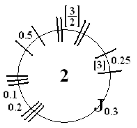
Figure 1. Exemplary designations to obtain the transition function described by Equation (11).

For the second type of transition functions, connections between nodes play a vital role. The branch between the $i\mathrm{th}$ and $j\mathrm{th}$ nodes has a value ${\mu }_{i,j}={\mu }_{j,i}$ and order $m_{i,j}=m_{j,i}$; whereas, if there is no connection between the $i\mathrm{th}$ and $j\mathrm{th}$ nodes, the branch has a value ${\mu }_{i,j}={\mu }_{j,i}=0$ (line order $m_{i,j}$ does not matter in such a case). It is also assumed that ${\mu }_{i,i}=1$ and $m_{i,i}=1$.

The types of lines are specified, which differ in line functions $f{l}_{i,j}$ (where i is the number of nodes, from which line function “was called”). These functions are defined in the remaining part of the paper, and their connections with scheme designations are described in Table 3. Line functions $f{l}_{i,j}$ will be used in both transition and measurement functions. If anywhere, $f{l}_{i,i}$ occurs (e.g., in Equation (17)), it is assumed that the first type of line function should be used, and all line parameters are the default.

$$f{l}_{i,j}^{\left(k\right)}=\{\begin{array}{ll}{\left(x_j^{\left(k\right)}\right)}^{m_{i,j}}·{\mu }_{i,j}& \mathrm{for} m_{i,j}\in \mathcal{Z}\\ {\left|x_j^{\left(k\right)}\right|}^{m_{i,j}}·{\mu }_{i,j}& \mathrm{for} m_{i,j}\notin \mathcal{Z}\end{array}$$

(12)

$$f{l}_{i,j}^{\left(k\right)}=\{\begin{array}{ll}sin\left({\left(x_j^{\left(k\right)}\right)}^{m_{i,j}}-x_i^{\left(k\right)}\right)·{\mu }_{i,j}& m_{i,j}\in \mathcal{Z}\\ sin\left({\left|x_j^{\left(k\right)}\right|}^{m_{i,j}}-x_i^{\left(k\right)}\right)·{\mu }_{i,j}& m_{i,j}\notin \mathcal{Z}\end{array}$$

(13)

$$f{l}_{i,j}^{\left(k\right)}=ln\left({\left|x_j^{\left(k\right)}\right|}^{m_{i,j}}+0.001\right)·{\mu }_{i,j}$$

(14)

Table 3. Explanation of designations: lines.

Equation	Line Designation	Explanation
(12)–(14)		Values $m_{i,j}$ and ${\mu }_{i,j}$ should be written on the scheme near the line center. Furthermore, information about the branch type, in the form of diagonal lines (one for (12), two for (13), and three for (14)) should be presented there. If one (or both) of the parameters ${\mu }_{i,j}$ and $m_{i,j}=1$ is omitted, it is assumed that its value is equal to 1. If branches in a whole grid are only of the first type, diagonal lines can be omitted.
-		To use another line function, one should draw a double line between nodes; however, this line function should be explained in the text.

The second type of transition functions (squares), which depend also on other state variables, are presented below, i.e., in Equations (15)–(18), and their designations are presented and described in Table 4.

$$x_i^{(k+1)}=\{\begin{array}{ll}\alpha {\left(x_i^{\left(k\right)}\right)}^n·{\displaystyle \sum _{\begin{array}{c}j=1\\ j\ne i\end{array}}^{N_x}}f{l}_{i,j}^{\left(k\right)}+v_i^{\left(k\right)}& n\in \mathcal{Z}\\ \alpha {\left|x_i^{\left(k\right)}\right|}^n·{\displaystyle \sum _{\begin{array}{c}j=1\\ j\ne i\end{array}}^{N_x}}f{l}_{i,j}^{\left(k\right)}+v_i^{\left(k\right)}& n\notin \mathcal{Z}\end{array}$$

(15)

$$x_i^{(k+1)}=\alpha ·\sum _{\begin{array}{c}j=1\\ j\ne i\end{array}}^{N_x}\frac{f{l}_{i,j}^{\left(k\right)}}{\beta +{\left|f{l}_{i,j}^{\left(k\right)}\right|}^n}+v_i^{\left(k\right)}$$

(16)

$$x_i^{(k+1)}=\alpha ·\sum _{\begin{array}{c}j=1\\ {\mu }_{i,j}\ne 0\end{array}}^{N_x}cos\left(f{l}_{i,j}^{\left(k\right)}·\beta k^n+\phi {[}^{\circ }]\right)+v_i^{\left(k\right)}$$

(17)

$$x_i^{(k+1)}=\{\begin{array}{ll}{f}_i\left(x_i^{\left(k\right)},{\mathbf{u}}^{\left(k\right)},k\right)+v_i^{\left(k\right)}& \mathrm{with} \mathrm{prob}.p_J\\ -f_i\left(x_i^{\left(k\right)},{\mathbf{u}}^{\left(k\right)},k\right)+v_i^{\left(k\right)}& \mathrm{with} \mathrm{prob}.1-p_J\end{array}$$

(18)

Table 4. Explanation of designations: nodes, Part 2; for transition functions, which are based also on other state variables.

Equation	Designation of Node	Explanation
(15)		The n value should be written inside a square bracket. If the $\alpha$ or n parameter is omitted, it is assumed that the omitted parameter is equal to 1.
(16) and (17)		When all three values are given, one must take into account that $\alpha$ should be written before $\beta$ (above or on the left side of $\beta$). If any parameter ($\alpha$, $\beta$, or n) is not presented on the scheme, it is assumed that it is equal to 1; however, one should keep in mind that $\beta$ can be omitted only if $\alpha$ is also omitted.
(17)		Parameter $\phi$ should always be presented in degrees (${}^{\circ }$) to be able to distinguish it from other values. Omitted $\phi$ means that it is equal to zero.
(18)		$p_J$ should be written outside of the square as J’s sub- or super-script (can be also from the left side). Omitted $p_J$ means that this value is equal to $0.5$.
-		To use another transition function (which must be explained in the text), a double square should be used.

It is also possible to combine both transition function types (circles and squares). An example is presented in Figure 2, and the appropriate transition function of the first state variable is written in Equation (19). To obtain the jump function (Equation (18)) for both types of transition function, the “J” mark and $p_J$ value should be given in the place where the square and circle are connected.

$$x_1^{(k+1)}=\{\begin{array}{l}20x_1^{\left(k\right)}·sin\left({\left(x_2^{\left(k\right)}\right)}^2-x_1^{\left(k\right)}\right)+\frac{5sin\left({\left(x_2^{\left(k\right)}\right)}^2-x_1^{\left(k\right)}\right)}{1+\sqrt{\left|5sin\left({\left(x_2^{\left(k\right)}\right)}^2-x_1^{\left(k\right)}\right)\right|}}+2{\left(x_1^{\left(k\right)}\right)}^3+v_1^{\left(k\right)}\\ \mathrm{with} \mathrm{prob}.0.2\\ 20x_1^{\left(k\right)}·sin\left({\left(x_2^{\left(k\right)}\right)}^2-x_1^{\left(k\right)}\right)+\frac{5sin\left({\left(x_2^{\left(k\right)}\right)}^2-x_1^{\left(k\right)}\right)}{1+\sqrt{\left|5sin\left({\left(x_2^{\left(k\right)}\right)}^2-x_1^{\left(k\right)}\right)\right|}}-2{\left(x_1^{\left(k\right)}\right)}^3+v_1^{\left(k\right)}\\ \mathrm{with} \mathrm{prob}.0.8\end{array}$$

(19)

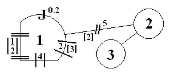
Figure 2. Exemplary designations to combine both types of transition functions; described by Equation (19).

Inputs should be presented by the element shown in Figure 3. The specific input signal should be presented inside the element, and as long as it is possible, all needed parameters for simulation should be described inside the input figure (see Figure 3).

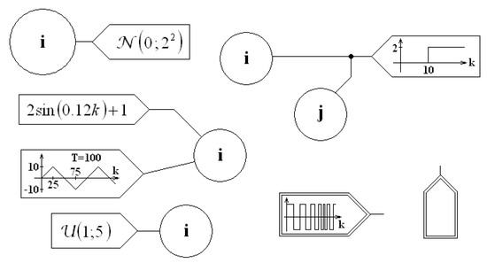
Figure 3. Exemplary input signal notation; the input signal should be presented as an arrow-shaped pentagon. As long as it is possible, the input signal should be integrally described inside the shape. If it is not possible, the pentagon should be doubled, and an explanation should be given in the text.

One state variable can have more than one input signal. If it is not obvious that the signal is periodic, one should insert information about the period length (in time steps), e.g., “$T=20$”. If all information about the input signal cannot be presented on the scheme, a double “input figure” should be used (examples are presented in Figure 3 on the right side).

The type of internal noise also should be presented on the scheme, or optionally, it should be described in the text. The PDF type with parameters should be connected to a specific node by a dashed line. Examples are presented in Figure 4.

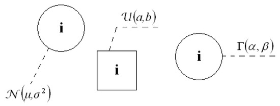
Figure 4. Internal noises should be marked on schemes using dashed lines that connect the distributions and nodes of state variables. Probability distributions should have specified parameters.

Measurements are presented on the scheme by filled marks. There are two types of measurements: nodal (associated with a specific node) and branch (associated with a specific line). The nodal measurement can depend on a state variable of this node and also on all state variables of the nodes that are connected with this node by lines. The branch measurement depends only on the two state variables of the two nodes that are connected by the line where the measurement is placed. In the case of branch measurements, one should keep in mind that the first index informs about near to which node a specific branch measurement is placed (branch measurements are not symmetric in general).

All nodal measurements proposed in the new network ($P_i$, $Q_i$, $R_i$, $S_i$, $T_i$) are described by (20)–(24), and examples of the designations on the scheme are presented in Table 5; whereas all proposed branch measurements are written by (25)–(29), and the exemplary designations are presented in Table 6.

$$P_i^{\left(k\right)}=z_o^{\left(k\right)}=\{\begin{array}{ll}\alpha {\left(x_i^{\left(k\right)}\right)}^{\lambda }+\gamma +n_o^{\left(k\right)}& \lambda \in \mathcal{Z}\\ \alpha {\left|x_i^{\left(k\right)}\right|}^{\lambda }+\gamma +n_o^{\left(k\right)}& \lambda \notin \mathcal{Z}\end{array}$$

(20)

$$Q_i^{\left(k\right)}=z_o^{\left(k\right)}=\alpha ·\prod _{\begin{array}{c}j=1\\ {\mu }_{i,j}\ne 0\end{array}}^{N_x}{x}_j^{\left(k\right)}{\mu }_{i,j}+n_o^{\left(k\right)}$$

(21)

$$R_i^{\left(k\right)}=z_o^{\left(k\right)}=\alpha ·\sum _{\begin{array}{c}j=1\\ j\ne i\end{array}}^{N_x}f{l}_{i,j}^{\left(k\right)}+n_o^{\left(k\right)}$$

(22)

$$S_i^{\left(k\right)}=z_o^{\left(k\right)}=\alpha x_i^{\left(k\right)}\sum _{j=1}^{N_x}{x}_j^{\left(k\right)}{\mu }_{i,j}·sin\left(x_i^{\left(k\right)}-x_j^{\left(k\right)}-{\mu }_{i,j}\right)+n_o^{\left(k\right)}$$

(23)

$$T_i^{\left(k\right)}=z_o^{\left(k\right)}=\alpha x_i^{\left(k\right)}\sum _{\begin{array}{c}j=1\\ j\ne i\end{array}}^{N_x}{x}_j^{\left(k\right)}{\mu }_{i,j}·cos\left(\frac{x_i^{\left(k\right)}-x_j^{\left(k\right)}}{ln\left(1.01+\left|f{l}_{i,j}^{\left(k\right)}\right|\right)}\right)+n_o^{\left(k\right)}$$

(24)

$$P_{i,j}^{\left(k\right)}=z_o^{\left(k\right)}=\alpha \left(x_i^{\left(k\right)}-x_j^{\left(k\right)}\right)+n_o^{\left(k\right)}$$

(25)

$$Q_{i,j}^{\left(k\right)}=z_o^{\left(k\right)}=\alpha ·x_i^{\left(k\right)}·x_j^{\left(k\right)}+n_o^{\left(k\right)}$$

(26)

$$R_{i,j}^{\left(k\right)}=z_o^{\left(k\right)}=\alpha \left(x_i^{\left(k\right)}+x_j^{\left(k\right)}·sin\left(\left(x_i^{\left(k\right)}+x_j^{\left(k\right)}\right)·f{l}_{i,j}^{\left(k\right)}\right)\right)+n_o^{\left(k\right)}$$

(27)

$$S_{i,j}^{\left(k\right)}=z_o^{\left(k\right)}=\alpha \left({\left(x_i^{\left(k\right)}\right)}^2-x_i^{\left(k\right)}{x}_j^{\left(k\right)}{\mu }_{i,j}·cos\left(x_i^{\left(k\right)}-x_j^{\left(k\right)}-{\mu }_{i,j}\right)\right)+n_o^{\left(k\right)}$$

(28)

$$T_{i,j}^{\left(k\right)}=z_o^{\left(k\right)}=\alpha ·\frac{max\left\{x_i^{\left(k\right)}+x_j^k;x_i^{\left(k\right)}·x_j^{\left(k\right)}\right\}}{0.01+\left|min\left\{{log}_2\left(0.01+\left|x_i^{\left(k\right)}{x}_j^{\left(k\right)}\right|\right);-0.1{\left(x_i^{\left(k\right)}+x_j^{\left(k\right)}\right)}^2+2\right\}\right|}·f{l}_{i,j}^{\left(k\right)}+n_o^{\left(k\right)}$$

(29)

Table 5. Explanation of designations: measurements, Part 1; for nodal measurements at the $i\mathrm{th}$ node.

Equation	Measurement Designation	Explanation
(20)		Value $\lambda$ should be always below or on the right side of the $\alpha$ parameter. If $\alpha$ or $\lambda$ are skipped, one can assume that they are equal to 1. However, if $\gamma$ is omitted, one should assume that $\gamma =0$. Parameter $\alpha$ can be skipped only if $\gamma$ is also omitted.
(21)		Nodal measurements should be placed near the node or should be connected with the node by the dashed line. In both cases, one can add information about measurement noise or the measurement scaling parameter ($\alpha$).
(22)
(23)
(24)

Table 6. Explanation of designations: measurements, Part 2; for branch measurements between the $i\mathrm{th}$ and $j\mathrm{th}$ nodes, but at the $i\mathrm{th}$ node.

Equation	Measurement Designation	Explanation
(25)		Branch measurements should be placed on the specific line. One should keep in mind that measurements are different at both ends of the branch, so the position of the mark should be unambiguous. For information about measurement noise or its scale parameter, a dashed line should be used.
(26)
(27)
(28)
(29)

The measurement noise should be marked in the same way as the internal noise: by a description in the text or using a dashed line on the scheme. Examples of measurement noise designations are presented in Table 5 and Table 6.

To use another measurement function, one can simply use a new filled mark on the scheme (such a function should be explained in the text).

2.2.1. Application for Power Systems

As was mentioned in the Introduction, the network described above can be created like the power system grid. Mainly, the S-type measurements were proposed based on the power flows and power injections, which occur in power systems. Below, 4 measurements from power grids with a description are presented; however, one should take into account that the notation presented in these equations absolutely cannot be associated with any markings of the rest of the paper (the notation is typical for the power system subject). The first two are power injections (active and reactive, respectively):

$$P_i\left(\mathbf{U},\delta \right)=\sum _{j=1}^B{U}_i{U}_j{Y}_{i,j}·cos\left({\delta }_i-{\delta }_j-{\mu }_{i,j}\right),$$

(30)

$$Q_i\left(\mathbf{U},\delta \right)=\sum _{j=1}^B{U}_i{U}_j{Y}_{i,j}·sin\left({\delta }_i-{\delta }_j-{\mu }_{i,j}\right),$$

(31)

and the two subsequent are power flows (active and reactive, respectively; in power flows, the first index informs about near to which bus (node) the measurement is placed):

$$P_{i,j}\left(\mathbf{U},\delta \right)=U_i^2{Y}_{i,j}·cos\left(-{\mu }_{i,j}\right)-U_i{U}_j{Y}_{i,j}·cos\left({\delta }_i-{\delta }_j-{\mu }_{i,j}\right),$$

(32)

$$Q_{i,j}\left(\mathbf{U},\delta \right)=U_i^2{Y}_{i,j}·sin\left(-{\mu }_{i,j}\right)-U_i{U}_j{Y}_{i,j}·sin\left({\delta }_i-{\delta }_j-{\mu }_{i,j}\right)+U_i^2\frac{y_{i,j}^{{}^{\prime }}}{2}.$$

(33)

In the above equations, B is the number of buses in a system. $Y_{i,j}$, ${\mu }_{i,j}$ and $y_{i,j}^{{}^{\prime }}$ are system parameters.

The state vector in power system grids is composed of voltage magnitudes $\mathbf{U}$ and phase angles $\delta$. One phasor (voltage magnitude and phase angle) is associated with every bus (node). Hence, it is visible that the length of the state vector is two times higher than the number of nodes (actually, the number of state variables is given by the $2B-1$ expression, because one node must be a reference node, in which the phase angle is constant, usually taken as 0).

The system composed only of S-type measurements (nodal and branch) and P-type measurements (nodal only) should successfully simulate the power system grid properties. Therefore, one can use a system created in such a way to speed up studies (due to the lower number of state variables), and after finding a promising method or algorithm, it can be checked on power systems.

The reader is directed to [32,33] for more information about power systems.

2.2.2. Exemplary Objects from the Literature

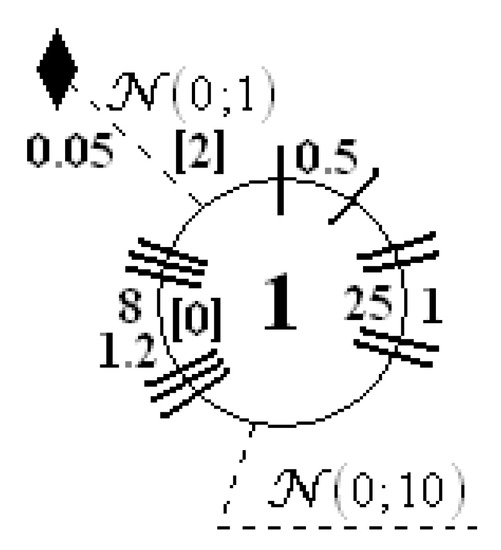
There are a few plants, which were used in literature, presented below. The first object is usually used in research associated with particle filters. It was proposed in 1978 by Netto, Gimeno, and Mendes (according to [34]). The object is a one-variable plant, the state space model of which is described by Equations (34)–(36). This model can be presented using the designations proposed in this paper, which one can see in Figure 5.

$$\{\begin{array}{l}{x}_1^{(k+1)}=0.5x_1^{\left(k\right)}+\frac{25x_1^{\left(k\right)}}{1+{\left(x_1^{\left(k\right)}\right)}^2}+8cos\left(1.2k\right)+v_1^{\left(k\right)}\\ z_1^{\left(k\right)}=\frac{{\left(x_1^{\left(k\right)}\right)}^2}{20}+n_1^{\left(k\right)}\end{array}$$

(34)

$$v_1^{\left(k\right)}\sim \mathcal{N}\left(0;10\right)$$

(35)

$$n_1^{\left(k\right)}\sim \mathcal{N}\left(0;1\right)$$

(36)

Figure 5. Scheme of the object, which was presented in [34] and described by Equations (34)–(36).

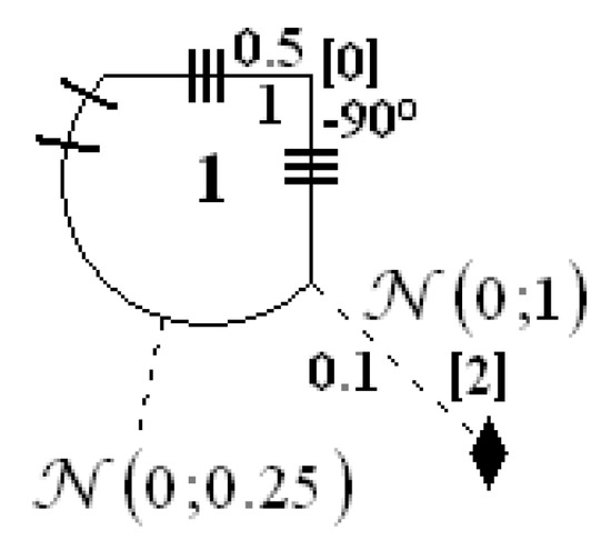
The second plant, described by Equations (37)–(39), was proposed in [35]. It can also be presented using the proposed designations, which is shown in Figure 6. This object was created based on the state Equation (34), but both (transition and measurement) functions were simplified.

$$\{\begin{array}{l}{x}_1^{(k+1)}=0.5x_1^{\left(k\right)}+\frac{25x_1^{\left(k\right)}}{1+{\left(x_1^{\left(k\right)}\right)}^2}+v_1^{\left(k\right)}\\ z_1^{\left(k\right)}=2x_1^{\left(k\right)}+n_1^{\left(k\right)}\end{array}$$

(37)

$$v_1^{\left(k\right)}\sim \mathcal{N}\left(0;10\right)$$

(38)

$$n_1^{\left(k\right)}\sim \mathcal{N}\left(0;100\right)$$

(39)

Figure 6. Scheme of the plant, which was presented in [35] and described by Equations (37)–(39).

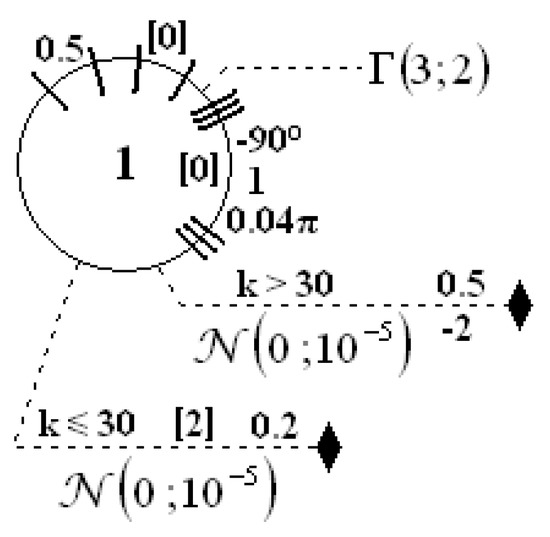
The subsequent object was used in [36] and is described by Equations (40)–(42). The description, using the proposed designations, is presented in Figure 7. As one can see, parameter $\phi =-{90}^{°}$ was used on the scheme to obtain “sin” instead of “cos” from Equation (17).

$$\{\begin{array}{l}{x}_1^{(k+1)}=x_1^{\left(k\right)}+0.5sin\left(x_1^{\left(k\right)}\right)+v_1^{\left(k\right)}\\ z_1^{\left(k\right)}=0.1{\left(x_1^{\left(k\right)}\right)}^2+n_1^{\left(k\right)}\end{array}$$

(40)

$$v_1^{\left(k\right)}\sim \mathcal{N}\left(0;0.25\right)$$

(41)

$$n_1^{\left(k\right)}\sim \mathcal{N}\left(0;1\right)$$

(42)

Figure 7. Scheme of the plant, which was presented in [36] and described by Equations (40)–(42).

The plant described by Equations (43)–(45) differs from other objects in such a way that its measurement function is switched after 30 time steps. It is marked in Figure 8 by two measurements, but with additional information, for the range of time steps for which it should be used. Moreover, the gamma PDF was used as internal noise.

$$\{\begin{array}{l}{x}_1^{(k+1)}=1+0.5x_1^{\left(k\right)}+sin\left(0.04\pi ·k\right)+v_1^{\left(k\right)}\\ z_1^{\left(k\right)}=\{\begin{array}{ll}0.2{\left(x_1^{\left(k\right)}\right)}^2+n_1^{\left(k\right)}& \mathrm{for}k\le 30\\ 0.5x_1^{\left(k\right)}-2+n_1^{\left(k\right)}& \mathrm{for}k>30\end{array}\end{array}$$

(43)

$$v_1^{\left(k\right)}\sim \mathsf{\Gamma }\left(3;2\right)$$

(44)

$$n_1^{\left(k\right)}\sim \mathcal{N}\left(0;{10}^{-5}\right)$$

(45)

Figure 8. Scheme of the object, which was presented in [37] and described by Equations (43)–(45).

The last object, which is mentioned below, was used in [38]. It is a tracking system, and its state-space model is given by Equation (46). The first two variables ($x_1$, $x_2$) are coordinates; the other two ($x_3$, $x_4$) are velocities; and the system scheme is presented in Figure 9. In the referenced article, the authors did not provide information about internal and measurement noises (it is only known that they were Gaussian). State variables $x_3$ and $x_4$ do not have internal noise, and this is why on the scheme, one can find “PDF” $\mathcal{U}(0;0)$.

$$\{\begin{array}{l}{x}_1^{(k+1)}=x_1^{\left(k\right)}+x_3^{\left(k\right)}+v_1^{\left(k\right)}\\ x_2^{(k+1)}=x_2^{\left(k\right)}+x_4^{\left(k\right)}+v_2^{\left(k\right)}\\ x_3^{(k+1)}=x_3^{\left(k\right)}\\ x_4^{(k+1)}=x_4^{\left(k\right)}\\ z_1^{\left(k\right)}=x_1^{\left(k\right)}+n_1^{\left(k\right)}\\ z_2^{\left(k\right)}=x_2^{\left(k\right)}+n_2^{\left(k\right)}\end{array}$$

(46)

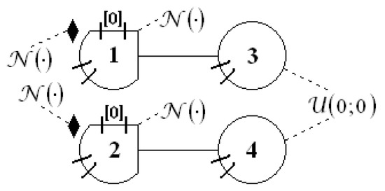
Figure 9. Scheme of the object, which was presented in [38] and described by Equation (46).

As was presented above, it is possible to model systems presented in the literature using the network proposed in this paper; however, one should keep in mind that the main goal was the easy creation of complex, multivariable, nonlinear systems, and not modeling the existing ones. Thanks to this, research on the plants with a network-type structure is possible with a relatively short state vector (number of state variables equal to the number of nodes).

2.2.3. Plants Used in the Experiments

The experiments were performed for the networks presented in Figure 10, Figure 11 and Figure 12. On all these schemes, there are no measurements; this is because they were considered in 5 different cases: P, Q, R, S, and T. In each case, the measurements were located in every possible place, but without repetitions (10 branch measurements and 4 nodal measurements). One can see an example in Figure 13: it is a S-type case for the $Ob402$ object.

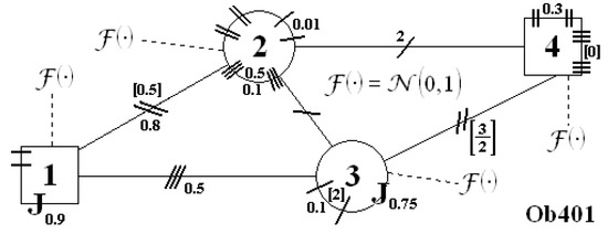
Figure 10. Scheme of the system $Ob401$.

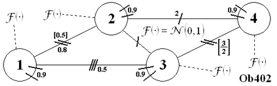
Figure 11. Scheme of the system $Ob402$.

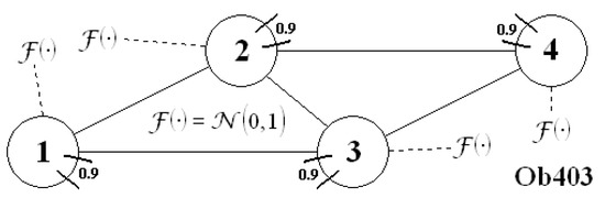
Figure 12. Scheme of the system $Ob403$.

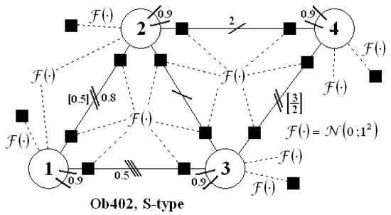
Figure 13. Scheme of the system $Ob402$ for the case with S-type measurements.

Finally, one should obtain 15 different systems; however, objects $Ob402$ and $Ob403$ had the same transition functions, and the difference was only in line functions $f{l}_{i,j}$ and in line parameters, which impacted the measurements; however, P-type measurements were identical for $Ob402$ and $Ob403$. Hence, the case with P-type measurements for $Ob402$ was omitted.

The transition function of these three systems is presented below: $Ob401$ is described by (47) and (48), and both objects, $Ob402$ and $Ob403$ are described by (49) and (50). All the measurement functions (for any case) one may find in the appendices: for system $Ob401$ in Appendix A, for system $Ob402$ in Appendix B (but the equations are the same as for $Ob401$) and for $Ob403$ plant in Appendix C (all measurements had default parameters: $\alpha =1$, $\lambda =1$, $\gamma =0$, $\phi =0^{\circ }$).

$$\{\begin{array}{l}{x}_1^{(k+1)}=\{\begin{array}{ll}0.8x_1^{\left(k\right)}sin\left({\left|x_2^{\left(k\right)}\right|}^{\frac{1}{2}}-x_1^{\left(k\right)}\right)+0.5x_1^{\left(k\right)}ln\left(0.001+\left|x_3^{\left(k\right)}\right|\right)+v_1^{\left(k\right)}& \mathrm{with} \mathrm{porob}.0.9\\ -0.8x_1^{\left(k\right)}sin\left({\left|x_2^{\left(k\right)}\right|}^{\frac{1}{2}}-x_1^{\left(k\right)}\right)-0.5x_1^{\left(k\right)}ln\left(0.001+\left|x_3^{\left(k\right)}\right|\right)+v_1^{\left(k\right)}& \mathrm{with} \mathrm{porob}.0.1\end{array}\\ x_2^{(k+1)}=0.01x_2^{\left(k\right)}+\frac{x_2^{\left(k\right)}}{1+x_2^{{\left(k\right)}^2}}+0.5x_2^{\left(k\right)}cos\left(0.1k\right)+v_2^{\left(k\right)}\\ x_3^{(k+1)}=\{\begin{array}{ll}0.1x_3^{{\left(k\right)}^2}+v_3^{\left(k\right)}& \mathrm{with} \mathrm{porob}.0.75\\ -0.1x_3^{{\left(k\right)}^2}+v_3^{\left(k\right)}& \mathrm{with} \mathrm{porob}.0.25\end{array}\\ x_4^{(k+1)}=\frac{2x_2^{\left(k\right)}}{0.3+\left|2x_2^{\left(k\right)}\right|}+\frac{sin\left({\left|x_3^{\left(k\right)}\right|}^{\frac{3}{2}}-x_4^{\left(k\right)}\right)}{0.3+\left|sin\left({\left|x_3^{\left(k\right)}\right|}^{\frac{3}{2}}-x_4^{\left(k\right)}\right)\right|}+\\ +cos\left(x_4^{\left(k\right)}\right)+cos\left(2x_2^{\left(k\right)}\right)+cos\left(sin\left({\left|x_3^{\left(k\right)}\right|}^{\frac{3}{2}}-x_4^{\left(k\right)}\right)\right)+v_4^{\left(k\right)}\end{array}$$

(47)

$$v_i\sim \mathcal{N}(0;1)\mathrm{for}i\in \{1,2,3,4\}$$

(48)

$$\{\begin{array}{l}{x}_1^{(k+1)}=0.9x_1^{\left(k\right)}+v_1^{\left(k\right)}\\ x_2^{(k+1)}=0.9x_2^{\left(k\right)}+v_2^{\left(k\right)}\\ x_3^{(k+1)}=0.9x_3^{\left(k\right)}+v_3^{\left(k\right)}\\ x_4^{(k+1)}=0.9x_4^{\left(k\right)}+v_4^{\left(k\right)}\end{array}$$

(49)

$$v_i\sim \mathcal{N}(0;1)\mathrm{for} i\in \{1,2,3,4\}$$

(50)

3. Results

The experiments were performed to check the dependence of the estimation quality on ESS and also on the complexity level of the transition and measurement functions.

The estimation quality was evaluated using the average root mean squared error, which is defined as:

$$\mathrm{aRMSE}=\frac{1}{N_x}\sum _{j=1}^{N_x}{\mathrm{RMSE}}_j=\frac{1}{N_x}\sum _{j=1}^{N_x}\sqrt{{\mathrm{MSE}}_j},$$

(51)

where $N_x$ is the number of state variables, and:

$$\sqrt{{\mathrm{MSE}}_j}=\sqrt{\frac{1}{M}\sum _{k=1}^M{\left({\hat{x}}_j^{\left(k\right)}-x_j^{\left(k\right)+}\right)}^2},$$

(52)

where x with a hat is the estimated state variable, x with a plus is the real value of state variable, and M is the simulation length (set on the 1000 time steps in all experiments). The aRMSE index can be used only for comparison; it does not make any physical sense. The lower the value of this index, the better the estimation quality.

Every experiment was different, values of the initial state vector (at zero time step) were drawn from uniform distribution $\mathcal{U}(-1;1)$. It was also assumed that initial values of particles were the same as the initial state vector.

All simulations were repeated until the standard deviation of the aRMSE mean value was less than 0.0025 (the variance of the mean value was s times smaller than the variance of s samples [39]), but at least 100 times. It was not achieved only for a few cases, which are mentioned in Table 7. Moreover, also for these cases, there were ranges on the charts, which showed, with 95% probability, where the mean value was placed (according to the 68-95-99.7 rule [40]). The results are presented in Figure 14, Figure 15, Figure 16 and Figure 17.

Table 7. Cases for which double standard deviations of the aRMSE mean values are presented in Figure 14 and Figure 15.

Object	Meas. Type	${\mathit{N}}_{\mathit{p}}$	Std. dev. of Mean
$Ob401$	Q	500	$0.0034$
$Ob401$	Q	1000	$0.0052$
$Ob401$	Q	1500	$0.0067$
$Ob401$	Q	2000	$0.0081$
$Ob401$	Q	3000	$0.0112$
$Ob401$	T	1500	$0.0026$
$Ob401$	T	2000	$0.0026$
$Ob401$	T	3000	$0.0040$

Figure 14. Obtained results: estimation quality based on the $\mathrm{aRMSE}$ index for plants with P-type, R-type, and T-type measurements.

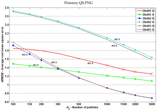
Figure 15. Obtained results: estimation quality based on the $\mathrm{aRMSE}$ index for plants with Q-type and S-type measurements.

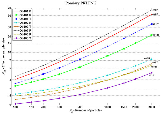
Figure 16. Obtained results: mean effective sample size (5) for plants with P-type, R-type, and T-type measurements.

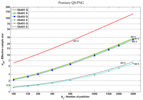
Figure 17. Obtained results: mean effective sample size (5) for plants with Q-type and S-type measurements.

4. Discussion and Further Work

As one can suppose, the lowest aRMSE values were obtained for the completely linear case $Ob403$-P (except the highest number of particles, where the $Ob403$-R case was the best). However, in general, the complexity level of equations (measurement or transition functions) had no impact on the estimation quality, or this influence was insignificant. In most of the cases, one could see the dependence: the greater the effective sample size, the better the estimation quality.

One could see that the results obtained for objects $Ob402$ and $Ob403$ in cases with Q-type and S-type measurements were almost the same. This was due to the fact that these systems were very similar (identical transition functions and measurement functions different only in system parameter ${\mu }_{i,j}$). In R-type and T-type measurement functions, the line functions $f{l}_{i,j}$ were used, which were very different between these two plants.

Based on the ESS results in Figure 16 and Figure 17, one can conclude that the number of particles $N_p$ impacted the ESS (higher $N_{eff}$ with higher $N_p$), but did not impact the order of cases (graphs did not intersect). It was also visible that ESS was relatively high for P-type measurements, which could have an impact on the good estimation quality.

The most interesting was probably the fact that the dependence “the more non-linear transition and measurement functions, the worse the estimation quality” was not always met. This was visible primarily for S-type measurements (see Figure 15): for the $Ob401$ system, the estimation quality was definitely better than for the two others. Similarly, in cases with T-type and R-type measurements (see Figure 14), a better estimation quality was obtained for the $Ob401$ system than for the $Ob402$ plant. Through all the experiments, the internal noise was the same. The following question arises: What was the reason for such results?

For almost all cases, one could see the relationship between the effective sample size and the estimation quality: the higher the $N_{eff}$, the lower the aRMSE. The $Ob401$-Q case was an exception: very high ESS (in comparison to other cases) resulted from the specificity of measurements (products of two or more state variables) and from the fact that for two state variables, “jumps” to the opposite values were possible (see Equation (47)). Consequently, although there was a relatively high number of significant particles in PF, a part of them was incorrect (with opposite signs).

However, the above-mentioned relationship was not satisfied for T-type and R-type measurements. Why was there the smallest ESS number for $Ob403$ systems, but simultaneously the best estimation quality was obtained (in comparison to the two other objects with the same measurements type)?

In these cases, the influence had a range of measurements, which one can see in Table 8. Variances of the subsequent measurements (from exemplary experiments) are presented in this table. A higher variance meant that, during the simulations, the values of that measurement changed more.

Table 8. Variances of the subsequent measurements during 100 experiments. The yellow background marks higher values in a column.

Meas. No.	R-Type			T-Type
	$\mathit{Ob}\mathbf{401}$	$\mathit{Ob}\mathbf{402}$	$\mathit{Ob}\mathbf{403}$	$\mathit{Ob}\mathbf{401}$	$\mathit{Ob}\mathbf{402}$	$\mathit{Ob}\mathbf{403}$
1	2.94	3.08	57.27	2.47	12.48	63.28
2	4.21	7.26	8.34	71.07	129.1	2851
3	4.23	7.41	8.32	22.82	90.51	2728
4	3.15	7.36	8.32	71.66	133.4	2958
5	23.72	140.5	82.57	12.64	74.91	68.64
6	2.2	8.19	8.28	301	3068	3029
7	3.63	8.03	8.15	14,397	9930	2751
8	2.82	7.46	8.25	47.59	92.81	2803
9	1.86	8.11	8.21	556	2851	2898
10	2.39	32.01	85.1	3.42	28.65	72.49
11	3.16	7.76	8.08	164.6	226.9	2861
12	4.23	7.96	8.07	3578	11,409	2921
13	3.78	7.82	8.05	167.3	224.2	2875
14	25.36	115	53.92	13.42	62.87	61.33

One should keep in mind that the measurement noises were the same (had the same distribution) during the experiments for all cases. The higher values the measurement had, the lower the impact the measurement noise had on the estimation process. As a result, the small $N_{eff}$ values in these cases were associated with more accurate measurements, and not with difficulties in state vector tracking.

This could be presented in a one-dimensional example with measurement function $z^{\left(k\right)}=a{x}^{\left(k\right)}+n^{\left(k\right)}$ ($n^{\left(k\right)}\sim \mathcal{N}(0,1)$). For smaller values of a, a higher value of ESS was obtained, whereas for a higher value of a, lower ESS, but in the latter case, particles with significant weights would be definitely closer to the sought value. An example is presented in Figure 18.

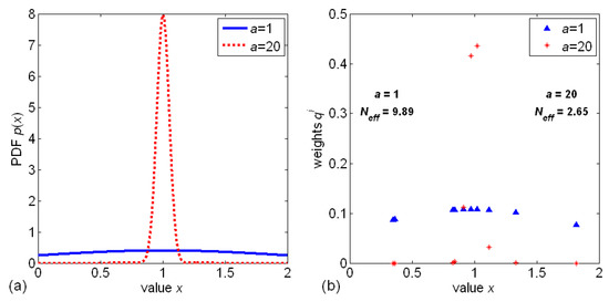
Figure 18. An example that shows the difference in weight values for measurement $z^{\left(k\right)}=a{x}^{\left(k\right)}+n^{\left(k\right)}$ ($n\sim \mathcal{N}(0,1)$). For $a=1$, measured value was assumed to be one, and for $a=20$, the measured value was assumed to be 20 (for better readability). (a) Exemplary probability density functions; (b) exemplary particles (with normalized weights) drawn from PDFs.

However, regardless of the considered case, one could notice a very low number of significant particles; in most cases from two to 30. How precisely will the four-dimensional PDF be modeled using even 30 points? Using 81 points, one would have accuracy similar to modeling a one-dimensional PDF by three points.

Therefore, the authors considered that further studies should be directed at ESS increasing, and the improvement of estimation quality would be only the result of these actions. They would be started with a comparison of different PF methods and resampling algorithms, in terms of state estimation quality and effective sample size in multivariable systems.

One possible solution may be the usage of an adaptive sample size [41]; however, this would only result in the increase of the particle number, as much as ESS would achieve a set threshold. Another method, which should improve the effective sample size, is the Population Monte Carlo (PMC) algorithm [42,43]. In this approach, it is assumed that particles are divided into a few groups and each one is drawn from different PDFs. Every PDF is calculated based on the drawn, up to this moment, particles and their weights. Yet another solution could be a double drawing: the first time locating an interesting area and the second time drawing mainly from this subspace. The authors are already working on a new PF algorithm that will be based on the latter approach.

The network proposed in this article had of course some disadvantages and limitations: the graphical representation of more complex systems with a higher number of nodes would be illegible (a description in the text would also be required). Despite the fact that many different options were proposed, the one was strongly limited in the creation of transition functions, and measurements were mostly non-parametric (only scale factor $\alpha$ was available). Furthermore, only additive noises were considered (could be also multiplicative and others).

Despite all these disadvantages, the authors believe that the proposed network was sufficient for a variety of particle filter studies, and not only this one. Additionally, for the main application (simulation of power grid behavior), it was totally suitable.

In the future, the authors will prepare and share the source code, which will allow performing experiments, not only for the networks presented in the article, but also for any other one (based on the external file with a system structure description).

Appendix A.1. Case for P-Type Measurements

$$P_1^{\left(k\right)}=x_1^{\left(k\right)}+n_1^{\left(k\right)}$$

(A1)

$$P_2^{\left(k\right)}=x_2^{\left(k\right)}+n_2^{\left(k\right)}$$

(A2)

$$P_3^{\left(k\right)}=x_3^{\left(k\right)}+n_3^{\left(k\right)}$$

(A3)

$$P_4^{\left(k\right)}=x_4^{\left(k\right)}+n_4^{\left(k\right)}$$

(A4)

$$P_{1,2}^{\left(k\right)}=x_1^{\left(k\right)}-x_2^{\left(k\right)}+n_5^{\left(k\right)}$$

(A5)

$$P_{1,3}^{\left(k\right)}=x_1^{\left(k\right)}-x_3^{\left(k\right)}+n_6^{\left(k\right)}$$

(A6)

$$P_{2,1}^{\left(k\right)}=x_2^{\left(k\right)}-x_1^{\left(k\right)}+n_7^{\left(k\right)}$$

(A7)

$$P_{2,3}^{\left(k\right)}=x_2^{\left(k\right)}-x_3^{\left(k\right)}+n_8^{\left(k\right)}$$

(A8)

$$P_{2,4}^{\left(k\right)}=x_2^{\left(k\right)}-x_4^{\left(k\right)}+n_9^{\left(k\right)}$$

(A9)

$$P_{3,1}^{\left(k\right)}=x_3^{\left(k\right)}-x_1^{\left(k\right)}+n_{10}^{\left(k\right)}$$

(A10)

$$P_{3,2}^{\left(k\right)}=x_3^{\left(k\right)}-x_2^{\left(k\right)}+n_{11}^{\left(k\right)}$$

(A11)

$$P_{3,4}^{\left(k\right)}=x_3^{\left(k\right)}-x_4^{\left(k\right)}+n_{12}^{\left(k\right)}$$

(A12)

$$P_{4,2}^{\left(k\right)}=x_4^{\left(k\right)}-x_2^{\left(k\right)}+n_{13}^{\left(k\right)}$$

(A13)

$$P_{4,3}^{\left(k\right)}=x_4^{\left(k\right)}-x_3^{\left(k\right)}+n_{14}^{\left(k\right)}$$

(A14)

$$n_i^{\left(k\right)}\sim \mathcal{N}\left(0;1^2\right)\mathrm{for} i\in \{1,\dots ,14\}$$

(A15)

Appendix A.2. Case for Q-Type Measurements

$$Q_1^{\left(k\right)}=0.4x_1^{\left(k\right)}{x}_2^{\left(k\right)}{x}_3^{\left(k\right)}+n_1^{\left(k\right)}$$

(A16)

$$Q_2^{\left(k\right)}=1.6x_1^{\left(k\right)}{x}_2^{\left(k\right)}{x}_3^{\left(k\right)}{x}_4^{\left(k\right)}+n_2^{\left(k\right)}$$

(A17)

$$Q_3^{\left(k\right)}=0.5x_1^{\left(k\right)}{x}_2^{\left(k\right)}{x}_3^{\left(k\right)}{x}_4^{\left(k\right)}+n_3^{\left(k\right)}$$

(A18)

$$Q_4^{\left(k\right)}=2x_2^{\left(k\right)}{x}_3^{\left(k\right)}{x}_4^{\left(k\right)}+n_4^{\left(k\right)}$$

(A19)

$$Q_{1,2}^{\left(k\right)}=x_1^{\left(k\right)}{x}_2^{\left(k\right)}+n_5^{\left(k\right)}$$

(A20)

$$Q_{1,3}^{\left(k\right)}=x_1^{\left(k\right)}{x}_3^{\left(k\right)}+n_6^{\left(k\right)}$$

(A21)

$$Q_{2,1}^{\left(k\right)}=x_2^{\left(k\right)}{x}_1^{\left(k\right)}+n_7^{\left(k\right)}$$

(A22)

$$Q_{2,3}^{\left(k\right)}=x_2^{\left(k\right)}{x}_3^{\left(k\right)}+n_8^{\left(k\right)}$$

(A23)

$$Q_{2,4}^{\left(k\right)}=x_2^{\left(k\right)}{x}_4^{\left(k\right)}+n_9^{\left(k\right)}$$

(A24)

$$Q_{3,1}^{\left(k\right)}=x_3^{\left(k\right)}{x}_1^{\left(k\right)}+n_{10}^{\left(k\right)}$$

(A25)

$$Q_{3,2}^{\left(k\right)}=x_3^{\left(k\right)}{x}_2^{\left(k\right)}+n_{11}^{\left(k\right)}$$

(A26)

$$Q_{3,4}^{\left(k\right)}=x_3^{\left(k\right)}{x}_4^{\left(k\right)}+n_{12}^{\left(k\right)}$$

(A27)

$$Q_{4,2}^{\left(k\right)}=x_4^{\left(k\right)}{x}_2^{\left(k\right)}+n_{13}^{\left(k\right)}$$

(A28)

$$Q_{4,3}^{\left(k\right)}=x_4^{\left(k\right)}{x}_3^{\left(k\right)}+n_{14}^{\left(k\right)}$$

(A29)

$$n_i^{\left(k\right)}\sim \mathcal{N}\left(0;1^2\right)\mathrm{for} i\in \{1,\dots ,14\}$$

(A30)

Appendix A.3. Case for R-Type Measurements

$$R_1^{\left(k\right)}=x_1^{\left(k\right)}\left(0.8sin\left({\left|x_2^{\left(k\right)}\right|}^{\frac{1}{2}}-x_1^{\left(k\right)}\right)+0.5ln\left(0.001+\left|x_3^{\left(k\right)}\right|\right)\right)+n_1^{\left(k\right)}$$

(A31)

$$R_2^{\left(k\right)}=x_2^{\left(k\right)}\left(0.8sin\left({\left|x_1^{\left(k\right)}\right|}^{\frac{1}{2}}-x_2^{\left(k\right)}\right)+x_3^{\left(k\right)}+2x_4^{\left(k\right)}\right)+n_2^{\left(k\right)}$$

(A32)

$$R_3^{\left(k\right)}=x_3^{\left(k\right)}\left(0.5ln\left(0.001+\left|x_1^{\left(k\right)}\right|\right)+x_2^{\left(k\right)}+sin\left({\left|x_4^{\left(k\right)}\right|}^{\frac{3}{2}}-x_3^{\left(k\right)}\right)\right)+n_3^{\left(k\right)}$$

(A33)

$$R_4^{\left(k\right)}=x_4^{\left(k\right)}\left(2x_2^{\left(k\right)}+sin\left({\left|x_3^{\left(k\right)}\right|}^{\frac{3}{2}}-x_4^{\left(k\right)}\right)\right)+n_4^{\left(k\right)}$$

(A34)

$$R_{1,2}^{\left(k\right)}=x_1^{\left(k\right)}+x_2^{\left(k\right)}sin\left(\left(x_1^{\left(k\right)}+x_2^{\left(k\right)}\right)·0.8sin\left({\left|x_2^{\left(k\right)}\right|}^{\frac{1}{2}}-x_1^{\left(k\right)}\right)\right)+n_5^{\left(k\right)}$$

(A35)

$$R_{1,3}^{\left(k\right)}=x_1^{\left(k\right)}+x_3^{\left(k\right)}sin\left(\left(x_1^{\left(k\right)}+x_3^{\left(k\right)}\right)·0.5ln\left(0.001+0.5\left|x_3^{\left(k\right)}\right|\right)\right)+n_6^{\left(k\right)}$$

(A36)

$$R_{2,1}^{\left(k\right)}=x_2^{\left(k\right)}+x_1^{\left(k\right)}sin\left(\left(x_2^{\left(k\right)}+x_1^{\left(k\right)}\right)·0.8sin\left({\left|x_1^{\left(k\right)}\right|}^{\frac{1}{2}}-x_2^{\left(k\right)}\right)\right)+n_7^{\left(k\right)}$$

(A37)

$$R_{2,3}^{\left(k\right)}=x_2^{\left(k\right)}+x_3^{\left(k\right)}·sin\left(\left(x_2^{\left(k\right)}+x_3^{\left(k\right)}\right)·x_3^{\left(k\right)}\right)+n_8^{\left(k\right)}$$

(A38)

$$R_{2,4}^{\left(k\right)}=x_2^{\left(k\right)}+x_4^{\left(k\right)}·sin\left(\left(x_2^{\left(k\right)}+x_4^{\left(k\right)}\right)·2x_4^{\left(k\right)}\right)+n_9^{\left(k\right)}$$

(A39)

$$R_{3,1}^{\left(k\right)}=x_3^{\left(k\right)}+x_1^{\left(k\right)}sin\left(\left(x_3^{\left(k\right)}+x_1^{\left(k\right)}\right)·0.5ln\left(0.001+\left|x_1^{\left(k\right)}\right|\right)\right)+n_{10}^{\left(k\right)}$$

(A40)

$$R_{3,2}^{\left(k\right)}=x_3^{\left(k\right)}+x_2^{\left(k\right)}·sin\left(\left(x_3^{\left(k\right)}+x_2^{\left(k\right)}\right)·x_2^{\left(k\right)}\right)+n_{11}^{\left(k\right)}$$

(A41)

$$R_{3,4}^{\left(k\right)}=x_3^{\left(k\right)}+x_4^{\left(k\right)}sin\left(\left(x_3^{\left(k\right)}+x_4^{\left(k\right)}\right)·sin\left({\left|x_4^{\left(k\right)}\right|}^{\frac{3}{2}}-x_3^{\left(k\right)}\right)\right)+n_{12}^{\left(k\right)}$$

(A42)

$$R_{4,2}^{\left(k\right)}=x_4^{\left(k\right)}+x_2^{\left(k\right)}·sin\left(\left(x_4^{\left(k\right)}+x_2^{\left(k\right)}\right)·2x_2^{\left(k\right)}\right)+n_{13}^{\left(k\right)}$$

(A43)

$$R_{4,3}^{\left(k\right)}=x_4^{\left(k\right)}+x_3^{\left(k\right)}sin\left(\left(x_4^{\left(k\right)}+x_3^{\left(k\right)}\right)·sin\left({\left|x_3^{\left(k\right)}\right|}^{\frac{3}{2}}-x_4^{\left(k\right)}\right)\right)+n_{14}^{\left(k\right)}$$

(A44)

$$n_i^{\left(k\right)}\sim \mathcal{N}\left(0;1^2\right)\mathrm{for} i\in \{1,\dots ,14\}$$

(A45)

Appendix A.4. Case for S-Type Measurements

$$\begin{array}{c}{S}_1^{\left(k\right)}={\left(x_1^{\left(k\right)}\right)}^{2}sin(-1)+0.8x_1^{\left(k\right)}{x}_2^{\left(k\right)}·sin\left(x_1^{\left(k\right)}-x_2^{\left(k\right)}-0.8\right)+\hfill \\ +0.5x_1^{\left(k\right)}{x}_3^{\left(k\right)}·sin\left(x_1^{\left(k\right)}-x_3^{\left(k\right)}-0.5\right)+n_1^{\left(k\right)}\end{array}$$

(A46)

$$\begin{array}{c}{S}_2^{\left(k\right)}=0.8x_2^{\left(k\right)}{x}_1^{\left(k\right)}sin\left(x_2^{\left(k\right)}-x_1^{\left(k\right)}-0.8\right)+{\left(x_2^{\left(k\right)}\right)}^{2}sin(-1)+x_2^{\left(k\right)}{x}_3^{\left(k\right)}sin\left(x_2^{\left(k\right)}-x_3^{\left(k\right)}-1\right)+\hfill \\ +2x_2^{\left(k\right)}{x}_4^{\left(k\right)}sin\left(x_2^{\left(k\right)}-x_4^{\left(k\right)}-2\right)+n_2^{\left(k\right)}\end{array}$$

(A47)

$$\begin{array}{c}{S}_3^{\left(k\right)}=0.5x_3^{\left(k\right)}{x}_1^{\left(k\right)}sin\left(x_3^{\left(k\right)}-x_1^{\left(k\right)}-0.5\right)+x_3^{\left(k\right)}{x}_2^{\left(k\right)}sin\left(x_3^{\left(k\right)}-x_2^{\left(k\right)}-1\right)+x_3^{{\left(k\right)}^2}sin(-1)+\hfill \\ +x_3^{\left(k\right)}{x}_4^{\left(k\right)}sin\left(x_3^{\left(k\right)}-x_4^{\left(k\right)}-1\right)+n_3^{\left(k\right)}\end{array}$$

(A48)

$$S_4^{\left(k\right)}=2x_4^{\left(k\right)}{x}_2^{\left(k\right)}sin\left(x_4^{\left(k\right)}-x_2^{\left(k\right)}-2\right)+x_4^{\left(k\right)}{x}_3^{\left(k\right)}sin\left(x_4^{\left(k\right)}-x_3^{\left(k\right)}-1\right)+x_4^{{\left(k\right)}^2}sin(-1)+n_4^{\left(k\right)}$$

(A49)

$$S_{1,2}^{\left(k\right)}=x_1^{{\left(k\right)}^2}-x_1^{\left(k\right)}{x}_2^{\left(k\right)}·0.8cos\left(x_1^{\left(k\right)}-x_2^{\left(k\right)}-0.8\right)+n_5^{\left(k\right)}$$

(A50)

$$S_{1,3}^{\left(k\right)}=x_1^{{\left(k\right)}^2}-x_1^{\left(k\right)}{x}_3^{\left(k\right)}·0.5cos\left(x_1^{\left(k\right)}-x_3^{\left(k\right)}-0.5\right)+n_6^{\left(k\right)}$$

(A51)

$$S_{2,1}^{\left(k\right)}=x_2^{{\left(k\right)}^2}-x_2^{\left(k\right)}{x}_1^{\left(k\right)}·0.8cos\left(x_2^{\left(k\right)}-x_1^{\left(k\right)}-0.8\right)+n_7^{\left(k\right)}$$

(A52)

$$S_{2,3}^{\left(k\right)}=x_2^{{\left(k\right)}^2}-x_2^{\left(k\right)}{x}_3^{\left(k\right)}·cos\left(x_2^{\left(k\right)}-x_3^{\left(k\right)}-1\right)+n_8^{\left(k\right)}$$

(A53)

$$S_{2,4}^{\left(k\right)}=x_2^{{\left(k\right)}^2}-x_2^{\left(k\right)}{x}_4^{\left(k\right)}·2cos\left(x_2^{\left(k\right)}-x_4^{\left(k\right)}-2\right)+n_9^{\left(k\right)}$$

(A54)

$$S_{3,1}^{\left(k\right)}=x_3^{{\left(k\right)}^2}-x_3^{\left(k\right)}{x}_1^{\left(k\right)}·0.5cos\left(x_3^{\left(k\right)}-x_1^{\left(k\right)}-0.5\right)+n_{10}^{\left(k\right)}$$

(A55)

$$S_{3,2}^{\left(k\right)}=x_3^{{\left(k\right)}^2}-x_3^{\left(k\right)}{x}_2^{\left(k\right)}·cos\left(x_3^{\left(k\right)}-x_2^{\left(k\right)}-1\right)+n_{11}^{\left(k\right)}$$

(A56)

$$S_{3,4}^{\left(k\right)}=x_3^{{\left(k\right)}^2}-x_3^{\left(k\right)}{x}_4^{\left(k\right)}·cos\left(x_3^{\left(k\right)}-x_4^{\left(k\right)}-1\right)+n_{12}^{\left(k\right)}$$

(A57)

$$S_{4,2}^{\left(k\right)}=x_4^{{\left(k\right)}^2}-x_4^{\left(k\right)}{x}_2^{\left(k\right)}·2cos\left(x_4^{\left(k\right)}-x_2^{\left(k\right)}-2\right)+n_{13}^{\left(k\right)}$$

(A58)

$$S_{4,3}^{\left(k\right)}=x_4^{{\left(k\right)}^2}-x_4^{\left(k\right)}{x}_3^{\left(k\right)}·cos\left(x_4^{\left(k\right)}-x_3^{\left(k\right)}-1\right)+n_{14}^{\left(k\right)}$$

(A59)

$$n_i^{\left(k\right)}\sim \mathcal{N}\left(0;1^2\right)\mathrm{for} i\in \{1,\dots ,14\}$$

(A60)

Appendix A.5. Case for T-Type Measurements

$$\begin{array}{c}{T}_1^{\left(k\right)}=0.8x_1^{\left(k\right)}{x}_2^{\left(k\right)}·cos\left(\frac{x_1^{\left(k\right)}-x_2^{\left(k\right)}}{ln\left(1.01+\left|0.8sin\left({\left|x_2^{\left(k\right)}\right|}^{\frac{1}{2}}-x_1^{\left(k\right)}\right)\right|\right)}\right)+\hfill \\ +0.5x_1^{\left(k\right)}{x}_3^{\left(k\right)}·cos\left(\frac{x_1^{\left(k\right)}-x_3^{\left(k\right)}}{ln\left(1.01+\left|0.5ln\left(0.001+\left|x_3^{\left(k\right)}\right|\right)\right|\right)}\right)+n_1^{\left(k\right)}\end{array}$$

(A61)

$$\begin{array}{c}{T}_2^{\left(k\right)}=0.8x_2^{\left(k\right)}{x}_1^{\left(k\right)}·cos\left(\frac{x_2^{\left(k\right)}-x_1^{\left(k\right)}}{ln\left(1.01+\left|0.8sin\left({\left|x_1^{\left(k\right)}\right|}^{\frac{1}{2}}-x_2^{\left(k\right)}\right)\right|\right)}\right)+\hfill \\ +x_2^{\left(k\right)}{x}_3^{\left(k\right)}·cos\left(\frac{x_2^{\left(k\right)}-x_3^{\left(k\right)}}{ln\left(1.01+\left|x_3^{\left(k\right)}\right|\right)}\right)+2x_2^{\left(k\right)}·x_4^{\left(k\right)}cos\left(\frac{x_2^{\left(k\right)}-x_4^{\left(k\right)}}{ln\left(1.01+\left|2x_4^{\left(k\right)}\right|\right)}\right)+n_2^{\left(k\right)}\end{array}$$

(A62)

$$\begin{array}{c}{T}_3^{\left(k\right)}=0.5x_3^{\left(k\right)}{x}_1^{\left(k\right)}·cos\left(\frac{x_3^{\left(k\right)}-x_1^{\left(k\right)}}{ln\left(1.01+\left|0.5ln\left(0.001+\left|x_1^{\left(k\right)}\right|\right)\right|\right)}\right)+\hfill \\ +x_3^{\left(k\right)}{x}_2^{\left(k\right)}cos\left(\frac{x_3^{\left(k\right)}-x_2^{\left(k\right)}}{ln\left(1.01+\left|x_2^{\left(k\right)}\right|\right)}\right)+x_3^{\left(k\right)}{x}_4^{\left(k\right)}·cos\left(\frac{x_3^{\left(k\right)}-x_4^{\left(k\right)}}{ln\left(1.01+\left|sin\left({\left|x_4^{\left(k\right)}\right|}^{\frac{3}{2}}-x_3^{\left(k\right)}\right)\right|\right)}\right)+n_3^{\left(k\right)}\end{array}$$

(A63)

$$\begin{array}{c}{T}_4^{\left(k\right)}=2x_4^{\left(k\right)}{x}_2^{\left(k\right)}cos\left(\frac{x_4^{\left(k\right)}-x_2^{\left(k\right)}}{ln\left(1.01+\left|2x_2^{\left(k\right)}\right|\right)}\right)+\hfill \\ +x_4^{\left(k\right)}{x}_3^{\left(k\right)}cos\left(\frac{x_4^{\left(k\right)}-x_3^{\left(k\right)}}{ln\left(1.01+\left|sin\left({\left|x_3^{\left(k\right)}\right|}^{\frac{3}{2}}-x_4^{\left(k\right)}\right)\right|\right)}\right)+n_4^{\left(k\right)}\end{array}$$

(A64)

$$T_{1,2}^{\left(k\right)}=\frac{max\left\{x_1^{\left(k\right)}+x_2^{\left(k\right)};x_1^{\left(k\right)}{x}_2^{\left(k\right)}\right\}·0.8sin\left(\sqrt{\left|x_2^{\left(k\right)}\right|}-x_1^{\left(k\right)}\right)}{0.01+|min\left\{{log}_2\left(0.01+\left|x_1^{\left(k\right)}{x}_2^{\left(k\right)}\right|\right);-0.1{\left(x_1^{\left(k\right)}+x_2^{\left(k\right)}\right)}^2+2\right\}|}+n_5^{\left(k\right)}$$

(A65)

$$T_{1,3}^{\left(k\right)}=\frac{max\left\{x_1^{\left(k\right)}+x_3^{\left(k\right)};x_1^{\left(k\right)}{x}_3^{\left(k\right)}\right\}·0.5ln\left(0.001+\left|x_3^{\left(k\right)}\right|\right)}{0.01+|min\left\{{log}_2\left(0.01+\left|x_1^{\left(k\right)}{x}_3^{\left(k\right)}\right|\right);-0.1{\left(x_1^{\left(k\right)}+x_3^{\left(k\right)}\right)}^2+2\right\}|}+n_6^{\left(k\right)}$$

(A66)

$$T_{2,1}^{\left(k\right)}=\frac{max\left\{x_2^{\left(k\right)}+x_1^{\left(k\right)};x_2^{\left(k\right)}{x}_1^{\left(k\right)}\right\}·0.8sin\left({\left|x_1^{\left(k\right)}\right|}^{\frac{1}{2}}-x_2^{\left(k\right)}\right)}{0.01+|min\left\{{log}_2\left(0.01+\left|x_2^{\left(k\right)}{x}_1^{\left(k\right)}\right|\right);-0.1{\left(x_2^{\left(k\right)}+x_1^{\left(k\right)}\right)}^2+2\right\}|}+n_7^{\left(k\right)}$$

(A67)

$$T_{2,3}^{\left(k\right)}=\frac{max\left\{x_2^{\left(k\right)}+x_3^{\left(k\right)};x_2^{\left(k\right)}{x}_3^{\left(k\right)}\right\}·x_3^{\left(k\right)}}{0.01+|min\left\{{log}_2\left(0.01+\left|x_2^{\left(k\right)}{x}_3^{\left(k\right)}\right|\right);-0.1{\left(x_2^{\left(k\right)}+x_3^{\left(k\right)}\right)}^2+2\right\}|}+n_8^{\left(k\right)}$$

(A68)

$$T_{2,4}^{\left(k\right)}=\frac{max\left\{x_2^{\left(k\right)}+x_4^{\left(k\right)};x_2^{\left(k\right)}{x}_4^{\left(k\right)}\right\}·2x_4^{\left(k\right)}}{0.01+|min\left\{{log}_2\left(0.01+\left|x_2^{\left(k\right)}{x}_4^{\left(k\right)}\right|\right);-0.1{\left(x_2^{\left(k\right)}+x_4^{\left(k\right)}\right)}^2+2\right\}|}+n_9^{\left(k\right)}$$

(A69)

$$T_{3,1}^{\left(k\right)}=\frac{max\left\{x_3^{\left(k\right)}+x_1^{\left(k\right)};x_3^{\left(k\right)}{x}_1^{\left(k\right)}\right\}·0.5ln\left(0.001+\left|x_1^{\left(k\right)}\right|\right)}{0.01+|min\left\{{log}_2\left(0.01+\left|x_3^{\left(k\right)}{x}_1^{\left(k\right)}\right|\right);-0.1{\left(x_3^{\left(k\right)}+x_1^{\left(k\right)}\right)}^2+2\right\}|}+n_{10}^{\left(k\right)}$$

(A70)

$$T_{3,2}^{\left(k\right)}=\frac{max\left\{x_3^{\left(k\right)}+x_2^{\left(k\right)};x_3^{\left(k\right)}{x}_2^{\left(k\right)}\right\}·x_2^{\left(k\right)}}{0.01+|min\left\{{log}_2\left(0.01+\left|x_3^{\left(k\right)}{x}_2^{\left(k\right)}\right|\right);-0.1{\left(x_3^{\left(k\right)}+x_2^{\left(k\right)}\right)}^2+2\right\}|}+n_{11}^{\left(k\right)}$$

(A71)

$$T_{3,4}^{\left(k\right)}=\frac{max\left\{x_3^{\left(k\right)}+x_4^{\left(k\right)};x_3^{\left(k\right)}{x}_4^{\left(k\right)}\right\}·sin\left({\left|x_4^{\left(k\right)}\right|}^{\frac{3}{2}}-x_3^{\left(k\right)}\right)}{0.01+|min\left\{{log}_2\left(0.01+\left|x_3^{\left(k\right)}{x}_4^{\left(k\right)}\right|\right);-0.1{\left(x_3^{\left(k\right)}+x_4^{\left(k\right)}\right)}^2+2\right\}|}+n_{12}^{\left(k\right)}$$

(A72)

$$T_{4,2}^{\left(k\right)}=\frac{max\left\{x_4^{\left(k\right)}+x_2^{\left(k\right)};x_4^{\left(k\right)}{x}_2^{\left(k\right)}\right\}·2x_2^{\left(k\right)}}{0.01+|min\left\{{log}_2\left(0.01+\left|x_4^{\left(k\right)}{x}_2^{\left(k\right)}\right|\right);-0.1{\left(x_4^{\left(k\right)}+x_2^{\left(k\right)}\right)}^2+2\right\}|}+n_{13}^{\left(k\right)}$$

(A73)

$$T_{4,3}^{\left(k\right)}=\frac{max\left\{x_4^{\left(k\right)}+x_3^{\left(k\right)};x_4^{\left(k\right)}{x}_3^{\left(k\right)}\right\}·sin\left({\left|x_3^{\left(k\right)}\right|}^{\frac{3}{2}}-x_4^{\left(k\right)}\right)}{0.01+|min\left\{{log}_2\left(0.01+\left|x_4^{\left(k\right)}{x}_3^{\left(k\right)}\right|\right);-0.1{\left(x_4^{\left(k\right)}+x_3^{\left(k\right)}\right)}^2+2\right\}|}+n_{14}^{\left(k\right)}$$

(A74)

$$n_i^{\left(k\right)}\sim \mathcal{N}\left(0;1^2\right)\mathrm{for} i\in \{1,\dots ,14\}$$

(A75)

Appendix C.1. Case for P-Type Measurements

$$P_1^{\left(k\right)}=x_1^{\left(k\right)}+n_1^{\left(k\right)}$$

(A76)

$$P_2^{\left(k\right)}=x_2^{\left(k\right)}+n_2^{\left(k\right)}$$

(A77)

$$P_3^{\left(k\right)}=x_3^{\left(k\right)}+n_3^{\left(k\right)}$$

(A78)

$$P_4^{\left(k\right)}=x_4^{\left(k\right)}+n_4^{\left(k\right)}$$

(A79)

$$P_{1,2}^{\left(k\right)}=x_1^{\left(k\right)}-x_2^{\left(k\right)}+n_5^{\left(k\right)}$$

(A80)

$$P_{1,3}^{\left(k\right)}=x_1^{\left(k\right)}-x_3^{\left(k\right)}+n_6^{\left(k\right)}$$

(A81)

$$P_{2,1}^{\left(k\right)}=x_2^{\left(k\right)}-x_1^{\left(k\right)}+n_7^{\left(k\right)}$$

(A82)

$$P_{2,3}^{\left(k\right)}=x_2^{\left(k\right)}-x_3^{\left(k\right)}+n_8^{\left(k\right)}$$

(A83)

$$P_{2,4}^{\left(k\right)}=x_2^{\left(k\right)}-x_4^{\left(k\right)}+n_9^{\left(k\right)}$$

(A84)

$$P_{3,1}^{\left(k\right)}=x_3^{\left(k\right)}-x_1^{\left(k\right)}+n_{10}^{\left(k\right)}$$

(A85)

$$P_{3,2}^{\left(k\right)}=x_3^{\left(k\right)}-x_2^{\left(k\right)}+n_{11}^{\left(k\right)}$$

(A86)

$$P_{3,4}^{\left(k\right)}=x_3^{\left(k\right)}-x_4^{\left(k\right)}+n_{12}^{\left(k\right)}$$

(A87)

$$P_{4,2}^{\left(k\right)}=x_4^{\left(k\right)}-x_2^{\left(k\right)}+n_{13}^{\left(k\right)}$$

(A88)

$$P_{4,3}^{\left(k\right)}=x_4^{\left(k\right)}-x_3^{\left(k\right)}+n_{14}^{\left(k\right)}$$

(A89)

$$n_i^{\left(k\right)}\sim \mathcal{N}\left(0;1^2\right)\mathrm{for} i\in \{1,\dots ,14\}$$

(A90)

Appendix C.2. Case for Q-Type Measurements

$$Q_1^{\left(k\right)}=x_1^{\left(k\right)}{x}_2^{\left(k\right)}{x}_3^{\left(k\right)}+n_1^{\left(k\right)}$$

(A91)

$$Q_2^{\left(k\right)}=x_1^{\left(k\right)}{x}_2^{\left(k\right)}{x}_3^{\left(k\right)}{x}_4^{\left(k\right)}+n_2^{\left(k\right)}$$

(A92)

$$Q_3^{\left(k\right)}=x_1^{\left(k\right)}{x}_2^{\left(k\right)}{x}_3^{\left(k\right)}{x}_4^{\left(k\right)}+n_3^{\left(k\right)}$$

(A93)

$$Q_4^{\left(k\right)}=x_2^{\left(k\right)}{x}_3^{\left(k\right)}{x}_4^{\left(k\right)}+n_4^{\left(k\right)}$$

(A94)

$$Q_{1,2}^{\left(k\right)}=x_1^{\left(k\right)}{x}_2^{\left(k\right)}+n_5^{\left(k\right)}$$

(A95)

$$Q_{1,3}^{\left(k\right)}=x_1^{\left(k\right)}{x}_3^{\left(k\right)}+n_6^{\left(k\right)}$$

(A96)

$$Q_{2,1}^{\left(k\right)}=x_2^{\left(k\right)}{x}_1^{\left(k\right)}+n_7^{\left(k\right)}$$

(A97)

$$Q_{2,3}^{\left(k\right)}=x_2^{\left(k\right)}{x}_3^{\left(k\right)}+n_8^{\left(k\right)}$$

(A98)

$$Q_{2,4}^{\left(k\right)}=x_2^{\left(k\right)}{x}_4^{\left(k\right)}+n_9^{\left(k\right)}$$

(A99)

$$Q_{3,1}^{\left(k\right)}=x_3^{\left(k\right)}{x}_1^{\left(k\right)}+n_{10}^{\left(k\right)}$$

(A100)

$$Q_{3,2}^{\left(k\right)}=x_3^{\left(k\right)}{x}_2^{\left(k\right)}+n_{11}^{\left(k\right)}$$

(A101)

$$Q_{3,4}^{\left(k\right)}=x_3^{\left(k\right)}{x}_4^{\left(k\right)}+n_{12}^{\left(k\right)}$$

(A102)

$$Q_{4,2}^{\left(k\right)}=x_4^{\left(k\right)}{x}_2^{\left(k\right)}+n_{13}^{\left(k\right)}$$

(A103)

$$Q_{4,3}^{\left(k\right)}=x_4^{\left(k\right)}{x}_3^{\left(k\right)}+n_{14}^{\left(k\right)}$$

(A104)

$$n_i^{\left(k\right)}\sim \mathcal{N}\left(0;1^2\right)\mathrm{for} i\in \{1,\dots ,14\}$$

(A105)

Appendix C.3. Case for R-Type Measurements

$$R_1^{\left(k\right)}=x_1^{\left(k\right)}\left(x_2^{\left(k\right)}+x_3^{\left(k\right)}\right)+n_1^{\left(k\right)}$$

(A106)

$$R_2^{\left(k\right)}=x_2^{\left(k\right)}\left(x_1^{\left(k\right)}+x_3^{\left(k\right)}+x_4^{\left(k\right)}\right)+n_2^{\left(k\right)}$$

(A107)

$$R_3^{\left(k\right)}=x_3^{\left(k\right)}\left(x_1^{\left(k\right)}+x_2^{\left(k\right)}+x_4^{\left(k\right)}\right)+n_3^{\left(k\right)}$$

(A108)

$$R_4^{\left(k\right)}=x_4^{\left(k\right)}\left(x_2^{\left(k\right)}+x_3^{\left(k\right)}\right)+n_4^{\left(k\right)}$$

(A109)

$$R_{1,2}^{\left(k\right)}=x_1^{\left(k\right)}+x_2^{\left(k\right)}·sin\left(\left(x_1^{\left(k\right)}+x_2^{\left(k\right)}\right)x_2^{\left(k\right)}\right)+n_5^{\left(k\right)}$$

(A110)

$$R_{1,3}^{\left(k\right)}=x_1^{\left(k\right)}+x_3^{\left(k\right)}·sin\left(\left(x_1^{\left(k\right)}+x_3^{\left(k\right)}\right)x_3^{\left(k\right)}\right)+n_6^{\left(k\right)}$$

(A111)

$$R_{2,1}^{\left(k\right)}=x_2^{\left(k\right)}+x_1^{\left(k\right)}·sin\left(\left(x_2^{\left(k\right)}+x_1^{\left(k\right)}\right)x_1^{\left(k\right)}\right)+n_7^{\left(k\right)}$$

(A112)

$$R_{2,3}^{\left(k\right)}=x_2^{\left(k\right)}+x_3^{\left(k\right)}·sin\left(\left(x_2^{\left(k\right)}+x_3^{\left(k\right)}\right)x_3^{\left(k\right)}\right)+n_8^{\left(k\right)}$$

(A113)

$$R_{2,4}^{\left(k\right)}=x_2^{\left(k\right)}+x_4^{\left(k\right)}·sin\left(\left(x_2^{\left(k\right)}+x_4^{\left(k\right)}\right)x_4^{\left(k\right)}\right)+n_9^{\left(k\right)}$$

(A114)

$$R_{3,1}^{\left(k\right)}=x_3^{\left(k\right)}+x_1^{\left(k\right)}·sin\left(\left(x_3^{\left(k\right)}+x_1^{\left(k\right)}\right)x_1^{\left(k\right)}\right)+n_{10}^{\left(k\right)}$$

(A115)

$$R_{3,2}^{\left(k\right)}=x_3^{\left(k\right)}+x_2^{\left(k\right)}·sin\left(\left(x_3^{\left(k\right)}+x_2^{\left(k\right)}\right)x_2^{\left(k\right)}\right)+n_{11}^{\left(k\right)}$$

(A116)

$$R_{3,4}^{\left(k\right)}=x_3^{\left(k\right)}+x_4^{\left(k\right)}·sin\left(\left(x_3^{\left(k\right)}+x_4^{\left(k\right)}\right)x_4^{\left(k\right)}\right)+n_{12}^{\left(k\right)}$$

(A117)

$$R_{4,2}^{\left(k\right)}=x_4^{\left(k\right)}+x_2^{\left(k\right)}·sin\left(\left(x_4^{\left(k\right)}+x_2^{\left(k\right)}\right)x_2^{\left(k\right)}\right)+n_{13}^{\left(k\right)}$$

(A118)

$$R_{4,3}^{\left(k\right)}=x_4^{\left(k\right)}+x_3^{\left(k\right)}·sin\left(\left(x_4^{\left(k\right)}+x_3^{\left(k\right)}\right)x_3^{\left(k\right)}\right)+n_{14}^{\left(k\right)}$$

(A119)

$$n_i^{\left(k\right)}\sim \mathcal{N}\left(0;1^2\right)\mathrm{for} i\in \{1,\dots ,14\}$$

(A120)

Appendix C.4. Case for S-Type Measurements

$$S_1^{\left(k\right)}=x_1^{{\left(k\right)}^2}sin(-1)+x_1^{\left(k\right)}{x}_2^{\left(k\right)}sin\left(x_1^{\left(k\right)}-x_2^{\left(k\right)}-1\right)+x_1^{\left(k\right)}{x}_3^{\left(k\right)}sin\left(x_1^{\left(k\right)}-x_3^{\left(k\right)}-1\right)+n_1^{\left(k\right)}$$

(A121)

$$\begin{array}{c}{S}_2^{\left(k\right)}=x_2^{\left(k\right)}{x}_1^{\left(k\right)}sin\left(x_2^{\left(k\right)}-x_1^{\left(k\right)}-1\right)+x_2^{{\left(k\right)}^2}sin(-1)+x_2^{\left(k\right)}{x}_3^{\left(k\right)}sin\left(x_2^{\left(k\right)}-x_3^{\left(k\right)}-1\right)+\hfill \\ +x_2^{\left(k\right)}{x}_4^{\left(k\right)}sin\left(x_2^{\left(k\right)}-x_4^{\left(k\right)}-1\right)+n_2^{\left(k\right)}\end{array}$$

(A122)

$$\begin{array}{c}{S}_3^{\left(k\right)}=x_3^{\left(k\right)}{x}_1^{\left(k\right)}sin\left(x_3^{\left(k\right)}-x_1^{\left(k\right)}-1\right)+x_3^{\left(k\right)}{x}_2^{\left(k\right)}sin\left(x_3^{\left(k\right)}-x_2^{\left(k\right)}-1\right)+x_3^{{\left(k\right)}^2}sin(-1)+\hfill \\ +x_3^{\left(k\right)}{x}_4^{\left(k\right)}sin\left(x_3^{\left(k\right)}-x_4^{\left(k\right)}-1\right)+n_3^{\left(k\right)}\end{array}$$

(A123)

$$S_4^{\left(k\right)}=x_4^{\left(k\right)}{x}_2^{\left(k\right)}sin\left(x_4^{\left(k\right)}-x_2^{\left(k\right)}-1\right)+x_4^{\left(k\right)}{x}_3^{\left(k\right)}sin\left(x_4^{\left(k\right)}-x_3^{\left(k\right)}-1\right)+x_4^{{\left(k\right)}^2}sin(-1)+n_4^{\left(k\right)}$$

(A124)

$$S_{1,2}^{\left(k\right)}=x_1^{{\left(k\right)}^2}-x_1^{\left(k\right)}{x}_2^{\left(k\right)}·cos\left(x_1^{\left(k\right)}-x_2^{\left(k\right)}-1\right)+n_5^{\left(k\right)}$$

(A125)

$$S_{1,3}^{\left(k\right)}=x_1^{{\left(k\right)}^2}-x_1^{\left(k\right)}{x}_3^{\left(k\right)}·cos\left(x_1^{\left(k\right)}-x_3^{\left(k\right)}-1\right)+n_6^{\left(k\right)}$$

(A126)

$$S_{2,1}^{\left(k\right)}=x_2^{{\left(k\right)}^2}-x_2^{\left(k\right)}{x}_1^{\left(k\right)}·cos\left(x_2^{\left(k\right)}-x_1^{\left(k\right)}-1\right)+n_7^{\left(k\right)}$$

(A127)

$$S_{2,3}^{\left(k\right)}=x_2^{{\left(k\right)}^2}-x_2^{\left(k\right)}{x}_3^{\left(k\right)}·cos\left(x_2^{\left(k\right)}-x_3^{\left(k\right)}-1\right)+n_8^{\left(k\right)}$$

(A128)

$$S_{2,4}^{\left(k\right)}=x_2^{{\left(k\right)}^2}-x_2^{\left(k\right)}{x}_4^{\left(k\right)}·cos\left(x_2^{\left(k\right)}-x_4^{\left(k\right)}-1\right)+n_9^{\left(k\right)}$$

(A129)

$$S_{3,1}^{\left(k\right)}=x_3^{{\left(k\right)}^2}-x_3^{\left(k\right)}{x}_1^{\left(k\right)}·cos\left(x_3^{\left(k\right)}-x_1^{\left(k\right)}-1\right)+n_{10}^{\left(k\right)}$$

(A130)

$$S_{3,2}^{\left(k\right)}=x_3^{{\left(k\right)}^2}-x_3^{\left(k\right)}{x}_2^{\left(k\right)}·cos\left(x_3^{\left(k\right)}-x_2^{\left(k\right)}-1\right)+n_{11}^{\left(k\right)}$$

(A131)

$$S_{3,4}^{\left(k\right)}=x_3^{{\left(k\right)}^2}-x_3^{\left(k\right)}{x}_4^{\left(k\right)}·cos\left(x_3^{\left(k\right)}-x_4^{\left(k\right)}-1\right)+n_{12}^{\left(k\right)}$$

(A132)

$$S_{4,2}^{\left(k\right)}=x_4^{{\left(k\right)}^2}-x_4^{\left(k\right)}{x}_2^{\left(k\right)}·cos\left(x_4^{\left(k\right)}-x_2^{\left(k\right)}-1\right)+n_{13}^{\left(k\right)}$$

(A133)

$$S_{4,3}^{\left(k\right)}=x_4^{{\left(k\right)}^2}-x_4^{\left(k\right)}{x}_3^{\left(k\right)}·cos\left(x_4^{\left(k\right)}-x_3^{\left(k\right)}-1\right)+n_{14}^{\left(k\right)}$$

(A134)

$$n_i^{\left(k\right)}\sim \mathcal{N}\left(0;1^2\right)\mathrm{for} i\in \{1,\dots ,14\}$$

(A135)

Appendix C.5. Case for T-Type Measurements

$$T_1^{\left(k\right)}=x_1^{\left(k\right)}{x}_2^{\left(k\right)}cos\left(\frac{x_1^{\left(k\right)}-x_2^{\left(k\right)}}{ln\left(1.01+\left|x_2^{\left(k\right)}\right|\right)}\right)+x_1^{\left(k\right)}{x}_3^{\left(k\right)}cos\left(\frac{x_1^{\left(k\right)}-x_3^{\left(k\right)}}{ln\left(1.01+\left|x_3^{\left(k\right)}\right|\right)}\right)+n_1^{\left(k\right)}$$

(A136)

$$\begin{array}{c}{T}_2^{\left(k\right)}=x_2^{\left(k\right)}{x}_1^{\left(k\right)}cos\left(\frac{x_2^{\left(k\right)}-x_1^{\left(k\right)}}{ln\left(1.01+\left|x_1^{\left(k\right)}\right|\right)}\right)+x_2^{\left(k\right)}{x}_3^{\left(k\right)}cos\left(\frac{x_2^{\left(k\right)}-x_3^{\left(k\right)}}{ln\left(1.01+\left|x_3^{\left(k\right)}\right|\right)}\right)+\hfill \\ +x_2^{\left(k\right)}{x}_4^{\left(k\right)}cos\left(\frac{x_2^{\left(k\right)}-x_4^{\left(k\right)}}{ln\left(1.01+\left|x_4^{\left(k\right)}\right|\right)}\right)+n_2^{\left(k\right)}\end{array}$$

(A137)

$$\begin{array}{c}{T}_3^{\left(k\right)}=x_3^{\left(k\right)}{x}_1^{\left(k\right)}cos\left(\frac{x_3^{\left(k\right)}-x_1^{\left(k\right)}}{ln\left(1.01+\left|x_1^{\left(k\right)}\right|\right)}\right)+x_3^{\left(k\right)}{x}_2^{\left(k\right)}cos\left(\frac{x_3^{\left(k\right)}-x_2^{\left(k\right)}}{ln\left(1.01+\left|x_2^{\left(k\right)}\right|\right)}\right)+\hfill \\ +x_3^{\left(k\right)}{x}_4^{\left(k\right)}cos\left(\frac{x_3^{\left(k\right)}-x_4^{\left(k\right)}}{ln\left(1.01+\left|x_4^{\left(k\right)}\right|\right)}\right)+n_3^{\left(k\right)}\end{array}$$

(A138)

$$T_4^{\left(k\right)}=x_4^{\left(k\right)}{x}_2^{\left(k\right)}cos\left(\frac{x_4^{\left(k\right)}-x_2^{\left(k\right)}}{ln\left(1.01+\left|x_2^{\left(k\right)}\right|\right)}\right)+x_4^{\left(k\right)}{x}_3^{\left(k\right)}cos\left(\frac{x_4^{\left(k\right)}-x_3^{\left(k\right)}}{ln\left(1.01+\left|x_3^{\left(k\right)}\right|\right)}\right)+n_4^{\left(k\right)}$$

(A139)

$$T_{1,2}^{\left(k\right)}=\frac{max\left\{x_1^{\left(k\right)}+x_2^{\left(k\right)};x_1^{\left(k\right)}{x}_2^{\left(k\right)}\right\}·x_2^{\left(k\right)}}{0.01+|min\left\{{log}_2\left(0.01+\left|x_1^{\left(k\right)}{x}_2^{\left(k\right)}\right|\right);-0.1{\left(x_1^{\left(k\right)}+x_2^{\left(k\right)}\right)}^2+2\right\}|}+n_5^{\left(k\right)}$$

(A140)

$$T_{1,3}^{\left(k\right)}=\frac{max\left\{x_1^{\left(k\right)}+x_3^{\left(k\right)};x_1^{\left(k\right)}{x}_3^{\left(k\right)}\right\}·x_3^{\left(k\right)}}{0.01+|min\left\{{log}_2\left(0.01+\left|x_1^{\left(k\right)}{x}_3^{\left(k\right)}\right|\right);-0.1{\left(x_1^{\left(k\right)}+x_3^{\left(k\right)}\right)}^2+2\right\}|}+n_6^{\left(k\right)}$$

(A141)

$$T_{2,1}^{\left(k\right)}=\frac{max\left\{x_2^{\left(k\right)}+x_1^{\left(k\right)};x_2^{\left(k\right)}{x}_1^{\left(k\right)}\right\}·x_1^{\left(k\right)}}{0.01+|min\left\{{log}_2\left(0.01+\left|x_2^{\left(k\right)}{x}_1^{\left(k\right)}\right|\right);-0.1{\left(x_2^{\left(k\right)}+x_1^{\left(k\right)}\right)}^2+2\right\}|}+n_7^{\left(k\right)}$$

(A142)

$$T_{2,3}^{\left(k\right)}=\frac{max\left\{x_2^{\left(k\right)}+x_3^{\left(k\right)};x_2^{\left(k\right)}{x}_3^{\left(k\right)}\right\}·x_3^{\left(k\right)}}{0.01+|min\left\{{log}_2\left(0.01+\left|x_2^{\left(k\right)}{x}_3^{\left(k\right)}\right|\right);-0.1{\left(x_2^{\left(k\right)}+x_3^{\left(k\right)}\right)}^2+2\right\}|}+n_8^{\left(k\right)}$$

(A143)

$$T_{2,4}^{\left(k\right)}=\frac{max\left\{x_2^{\left(k\right)}+x_4^{\left(k\right)};x_2^{\left(k\right)}{x}_4^{\left(k\right)}\right\}·x_4^{\left(k\right)}}{0.01+|min\left\{{log}_2\left(0.01+\left|x_2^{\left(k\right)}{x}_4^{\left(k\right)}\right|\right);-0.1{\left(x_2^{\left(k\right)}+x_4^{\left(k\right)}\right)}^2+2\right\}|}+n_9^{\left(k\right)}$$

(A144)

$$T_{3,1}^{\left(k\right)}=\frac{max\left\{x_3^{\left(k\right)}+x_1^{\left(k\right)};x_3^{\left(k\right)}{x}_1^{\left(k\right)}\right\}·x_1^{\left(k\right)}}{0.01+|min\left\{{log}_2\left(0.01+\left|x_3^{\left(k\right)}{x}_1^{\left(k\right)}\right|\right);-0.1{\left(x_3^{\left(k\right)}+x_1^{\left(k\right)}\right)}^2+2\right\}|}+n_{10}^{\left(k\right)}$$

(A145)

$$T_{3,2}^{\left(k\right)}=\frac{max\left\{x_3^{\left(k\right)}+x_2^{\left(k\right)};x_3^{\left(k\right)}{x}_2^{\left(k\right)}\right\}·x_2^{\left(k\right)}}{0.01+|min\left\{{log}_2\left(0.01+\left|x_3^{\left(k\right)}{x}_2^{\left(k\right)}\right|\right);-0.1{\left(x_3^{\left(k\right)}+x_2^{\left(k\right)}\right)}^2+2\right\}|}+n_{11}^{\left(k\right)}$$

(A146)

$$T_{3,4}^{\left(k\right)}=\frac{max\left\{x_3^{\left(k\right)}+x_4^{\left(k\right)};x_3^{\left(k\right)}{x}_4^{\left(k\right)}\right\}·x_4^{\left(k\right)}}{0.01+|min\left\{{log}_2\left(0.01+\left|x_3^{\left(k\right)}{x}_4^{\left(k\right)}\right|\right);-0.1{\left(x_3^{\left(k\right)}+x_4^{\left(k\right)}\right)}^2+2\right\}|}+n_{12}^{\left(k\right)}$$

(A147)

$$T_{4,2}^{\left(k\right)}=\frac{max\left\{x_4^{\left(k\right)}+x_2^{\left(k\right)};x_4^{\left(k\right)}{x}_2^{\left(k\right)}\right\}·x_2^{\left(k\right)}}{0.01+|min\left\{{log}_2\left(0.01+\left|x_4^{\left(k\right)}{x}_2^{\left(k\right)}\right|\right);-0.1{\left(x_4^{\left(k\right)}+x_2^{\left(k\right)}\right)}^2+2\right\}|}+n_{13}^{\left(k\right)}$$

(A148)

$$T_{4,3}^{\left(k\right)}=\frac{max\left\{x_4^{\left(k\right)}+x_3^{\left(k\right)};x_4^{\left(k\right)}{x}_3^{\left(k\right)}\right\}·x_3^{\left(k\right)}}{0.01+|min\left\{{log}_2\left(0.01+\left|x_4^{\left(k\right)}{x}_3^{\left(k\right)}\right|\right);-0.1{\left(x_4^{\left(k\right)}+x_3^{\left(k\right)}\right)}^2+2\right\}|}+n_{14}^{\left(k\right)}$$

(A149)

$$n_i^{\left(k\right)}\sim \mathcal{N}\left(0;1^2\right)\mathrm{for} i\in \{1,\dots ,14\}$$

(A150)

References

- Sutharsan, S.; Kirubarajan, T.; Lang, T.; McDonald, M. An Optimization-Based Parallel Particle Filter for Multitarget Tracking. IEEE Trans. Aerosp. Electron. Syst. 2012, 48, 1601–1618. [Google Scholar] [CrossRef]
- Doucet, A.; De Freitas, N.; Murphy, K.; Russell, S. Rao-Blackwellised particle filtering for dynamic Bayesian networks. In Proceedings of the Sixteenth Conference on Uncertainty in Artificial Intelligence; Morgan Kaufmann Publishers Inc.: Burlington, MA, USA, 2000; pp. 176–183. [Google Scholar]
- Hendeby, G.; Karlsson, R.; Gustafsson, F. The Rao-Blackwellized particle filter: A filter bank implementation. EURASIP J. Adv. Signal Process. 2010, 2010, 724087. [Google Scholar] [CrossRef]
- Šmídl, V.; Hofman, R. Marginalized particle filtering framework for tuning of ensemble filters. Mon. Weather Rev. 2011, 139, 3589–3599. [Google Scholar] [CrossRef]
- Djuric, P.M.; Lu, T.; Bugallo, M.F. Multiple particle filtering. In Proceedings of the 2007 IEEE International Conference on Acoustics, Speech and Signal Processing-ICASSP’07, Honolulu, HI, USA, 15–20 April 2007; Volume 3, pp. 1181–1184. [Google Scholar]
- Kozierski, P.; Lis, M.; Horla, D. Level of dispersion in dispersed particle filter. In Proceedings of the 20th International Conference on Methods and Models in Automation and Robotics (MMAR), Miedzyzdroje, Poland, 24–27 August 2015; pp. 418–423. [Google Scholar]
- Schweppe, F.C.; Wildes, J. Power system static-state estimation, Part I: Exact model. IEEE Trans. Power Appar. Syst. 1970, 89, 120–125. [Google Scholar] [CrossRef]
- Schweppe, F.C.; Rom, D.B. Power system static-state estimation, Part II: Approximate model. IEEE Trans. Power Appar. Syst. 1970, 89, 125–130. [Google Scholar] [CrossRef]
- Schweppe, F.C. Power system static-state estimation, Part III: Implementation. IEEE Trans. Power Appar. Syst. 1970, 89, 130–135. [Google Scholar] [CrossRef]
- Monticelli, A. Electric power system state estimation. Proc. IEEE 2000, 88, 262–282. [Google Scholar] [CrossRef]
- Wang, S.; Gao, W.; Meliopoulos, A.S. An alternative method for power system dynamic state estimation based on unscented transform. IEEE Trans. Power Syst. 2011, 27, 942–950. [Google Scholar] [CrossRef]
- Pandey, J.; Singh, D. Application of radial basis neural network for state estimation of power system networks. Int. J. Eng. Sci. Technol. 2010, 2, 19–28. [Google Scholar] [CrossRef]
- Udupa, H.N.; Minal, M.; Mishra, M.T. Node Level ANN Technique for Real Time Power System State Estimation. Int. J. Sci. Eng. Res. 2004, 5, 1500–1505. [Google Scholar]
- Chen, H.; Liu, X.; She, C.; Yao, C. Power System Dynamic State Estimation based on a New Particle Filter. Procedia Environ. Sci. 2011, 11, 655–661. [Google Scholar]
- Zhu, H.; Giannakis, G.B. Multi-area state estimation using distributed SDP for nonlinear power systems. In Proceedings of the 2012 IEEE Third International Conference on Smart Grid Communications (SmartGridComm), Tainan, Taiwan, 5–8 November 2012; pp. 623–628. [Google Scholar]
- Sharma, A.; Srivastava, S.; Chakrabarti, S. Multi area state estimation for smart grid application utilizing all SCADA and PMU measurements. In Proceedings of the 2014 IEEE Innovative Smart Grid Technologies-Asia (ISGT ASIA), Kuala Lumpur, Malaysia, 20–23 May 2014; pp. 525–530. [Google Scholar]
- Xie, L.; Choi, D.H.; Kar, S. Cooperative distributed state estimation: Local observability relaxed. In Proceedings of the 2011 IEEE Power and Energy Society General Meeting, Detroit, MI, USA, 24–28 July 2011; pp. 1–11. [Google Scholar]
- Guo, Y.; Wu, W.; Wang, Z.; Zhang, B.; Sun, H. A distributed power system state estimator incorporating linear and nonlinear areas. In Proceedings of the 2014 IEEE PES General Meeting Conference & Exposition, National Harbor, MD, USA, 27–31 July 2014; pp. 1–5. [Google Scholar]
- Kozierski, P.; Sadalla, T.; Owczarkowski, A.; Drgas, S. Particle filter in multidimensional systems. In Proceedings of the 21st International Conference on Methods and Models in Automation and Robotics (MMAR), Miedzyzdroje, Poland, 29 August–1 September 2016; pp. 806–810. [Google Scholar]
- Kozierski, P.; Michalski, J.; Sadalla, T.; Giernacki, W.; Zietkiewicz, J.; Drgas, S. New Grid for Particle Filtering of Multivariable Nonlinear Objects. In Proceedings of the 2018 Federated Conference on Computer Science and Information Systems (FedCSIS), Poznan, Poland, 9–12 September 2018; pp. 1073–1077. [Google Scholar]
- Candy, J.V. Bayesian Signal Processing; Wiley: Hoboken, NJ, USA, 2009; pp. 237–298. [Google Scholar]
- Gordon, J.N.; Salmond, D.J.; Smith, A.F.M. Novel Approach to Nonlinear/non-Gaussian Bayesian State Estimation. IEE Proc.-F 1993, 140, 107–113. [Google Scholar] [CrossRef]
- Li, F.; Wu, L.; Shi, P.; Lim, C.C. State Estimation and Sliding Mode Control for Semi-Markovian Jump Systems with Mismatched Uncertainties. Automatica 2015, 51, 385–393. [Google Scholar] [CrossRef]
- Kozierski, P.; Lis, M.; Zietkiewicz, J. Resampling in Particle Filtering–Comparison. Stud. Z Autom. I Inform. 2013, 38, 35–64. [Google Scholar]
- Brzozowska-Rup, K.; Dawidowicz, A.L. Particle filter method. Mat. Stosow. Mat. Dla Spoleczenstwa 2009, 10, 69–107. (In Polish) [Google Scholar]
- Yu, J.X.; Liu, W.J.; Tang, Y.L. Adaptive resampling in particle filter based on diversity measures. In Proceedings of the 2010 5th International Conference on Computer Science & Education, Hefei, China, 24–27 August 2010; pp. 1474–1478. [Google Scholar]
- Martino, L.; Elvira, V.; Louzada, F. Effective sample size for importance sampling based on discrepancy measures. Signal Process. 2017, 131, 386–401. [Google Scholar] [CrossRef]
- Arulampalam, S.; Maskell, S.; Gordon, N.; Clapp, T. A Tutorial on Particle Filters for On-line non-Linear/ non-Gaussian Bayesian Tracking. IEEE Trans. Signal Process. 2002, 50, 174–188. [Google Scholar] [CrossRef]
- Doucet, A.; Johansen, A.M. A Tutorial on Particle Filtering and Smoothing: Fifteen years later. Handb. Nonlinear Filter. 2009, 12, 3. [Google Scholar]
- Imtiaz, S.A.; Roy, K.; Huang, B.; Shah, S.L.; Jampana, P. Estimation of states of nonlinear systems using a particle filter. In Proceedings of the 2006 IEEE International Conference on Industrial Technology, Mumbai, India, 15–17 December 2006; pp. 2432–2437. [Google Scholar]
- Doucet, A.; De Freitas, N.; Gordon, N. An introduction to sequential Monte Carlo methods. In Sequential Monte Carlo Methods in Practice; Springer: New York, NY, USA, 2001; pp. 3–14. [Google Scholar]
- Abur, A.; Exposito, A.G. Power System State Estimation: Theory and Implementation; CRC Press: Boca Raton, FL, USA, 2004. [Google Scholar]
- Andersson, G. Modelling and Analysis of Electric Power Systems; EEH-Power Systems Laboratory, Swiss Federal Institute of Technology (ETH): Zürich, Switzerland, 2008. [Google Scholar]
- Kitagawa, G. Monte Carlo filter and smoother for non-Gaussian nonlinear state space models. J. Comput. Graph. Stat. 1996, 5, 1–25. [Google Scholar]
- Michalski, J.; Kozierski, P.; Zietkiewicz, J. Comparison of Particle Filter and Extended Kalman Particle Filter. Stud. Z. Autom. I Inform. 2017, 42, 43–51. [Google Scholar]
- Liu, X.; Wang, Y. The improved unscented Kalman particle filter based on MCMC and consensus strategy. In Proceedings of the 31st Chinese Control Conference, Hefei, China, 25–27 July 2012; pp. 6655–6658. [Google Scholar]
- Li, Q.; Sun, F. Adaptive cubature particle filter algorithm. In Proceedings of the 2013 IEEE International Conference on Mechatronics and Automation, Takamatsu, Japan, 4–7 Augusat 2013; pp. 1356–1360. [Google Scholar]
- Ha, S.V.U.; Jeon, J.W. Combine Kalman filter and particle filter to improve color tracking algorithm. In Proceedings of the 2007 International Conference on Control, Automation and Systems, Seoul, Korea, 17–20 October 2007; pp. 558–561. [Google Scholar]
- Plucinska, A.; Plucinski, E. Probabilistics Tasks; Panstwowe Wydawnictwo Naukowe: Warsaw, Poland, 1983. (In Polish) [Google Scholar]
- Florek, A.; Mazurkiewicz, P. Signals and Dynamic Systems; Wydawnictwo Politechniki Poznanskiej: Warsaw, Poznan, 2015. (In Polish) [Google Scholar]
- Straka, O.; Šimandl, M. Particle filter with adaptive sample size. Kybernetika 2011, 47, 385–400. [Google Scholar]
- Cappé, O.; Guillin, A.; Marin, J.M.; Robert, C.P. Population monte carlo. J. Comput. Graph. Stat. 2004, 13, 907–929. [Google Scholar] [CrossRef]
- Kozierski, P. Population Monte Carlo and Adaptive Importance Sampling in Particle Filter. Stud. Z Autom. I Inform. 2014, 39, 33–41. [Google Scholar]
© 2020 by the authors. Licensee MDPI, Basel, Switzerland. This article is an open access article distributed under the terms and conditions of the Creative Commons Attribution (CC BY) license (http://creativecommons.org/licenses/by/4.0/).