Assessment of Methods for the Real-Time Simulation of Electronic and Thermal Circuits

Abstract

Time–domain simulation of electronic and thermal circuits is required by a large array of applications, such as the design and optimization of electric vehicle powertrain components. While efficient execution is always a desirable feature of simulation codes, in certain cases like System-in-the-Loop setups, real-time performance is demanded. Whether real-time code execution can be achieved or not in a particular case depends on a series of factors, which include the mathematical formulation of the equations that govern the system dynamics, the techniques used in code implementation, and the capabilities of the hardware architecture on which the simulation is run. In this work, we present an evaluation framework of numerical methods for the simulation of electronic and thermal circuits from the point of view of their ability to deliver real-time performance. The methods were compared using a set of nontrivial benchmark problems and relevant error metrics. The computational efficiency of the simulation codes was measured under different software and hardware environments, to determine the feasibility of using them in industrial applications with reduced computational power.

1. Introduction

Computer simulation of dynamical systems is currently a necessary and often critical step in a large number of engineering applications. Accurate and efficient simulations enable considerable reductions in product development cycles, together with savings in prototyping and testing costs. The development of computing technologies in the latest decades has made it possible to extend the simulation of nontrivial engineering systems to real-time (RT) environments [1], including Hardware-in-the-Loop (HiL) and System-in-the-Loop (SITL) setups, in which computer simulations are interfaced to physical components. Such simulation processes often describe multiphysics systems of great complexity, composed by subsystems with very different behavior and physical properties. This task can be performed in an efficient way by means of co-simulation schemes, integrating the dynamics of each subsystem with its own dedicated solver, and coupling these through the exchange of a limited set of input and output variables [2,3,4,5]. This is the case of test benches in the automotive industry, in which physical components of a vehicle are interfaced to an RT simulation of the overall system, which may include mechanical, thermal, electronic, or hydraulic effects, as well as interactions with the driving environment. Test benches for e-powertrains, for instance, showcase the interest of developing effective simulation methods for circuits that represent engineering systems whose purpose is the management and control of energy flows in industrial applications [6].

Co-simulation in RT platforms requires that every subsystem in the assembly is able to complete the integration of its dynamics equations in real time. This is particularly critical in HiL and SITL environments, where the correct and safe performance of physical components depends on the inputs generated by the virtual ones being delivered in time. The time spent in computations by the virtual subsystems must, therefore, be predictable [7]. Such environments frequently require that the communication between subsystems takes place at fixed time intervals—moreover, using iterative coupling schemes to improve convergence is restricted by the presence of physical subsystems [8]. As a consequence, explicit coupling schemes with fixed communication step-sizes are the option of choice in RT co-simulation setups.

Electric and electronics subsystems are present in a wide range of multidisciplinary engineering applications, like electric vehicles. The numerical methods used for time–domain simulation of these circuits must meet the efficiency and accuracy requirements of the main application; in HiL and SITL setups, RT performance with fixed integration step-sizes is required. Time-domain computer-aided simulation of electric and electronic circuits has been the subject of research since the early 1970s [9,10]. Circuit dynamics is usually formulated in terms of a set of differential algebraic equations (DAE), resulting from the application of Kirchhoff laws and the constitutive equations of the circuit components, and integrated using numerical methods like the Newmark family of integrators [11] or backward differentiation formulas (BDF) [12]. The accuracy and stability of these methods have been assessed in a number of research papers and compared to alternative integration formulas such as implicit Runge–Kutta methods [13,14]. Some of these pay special attention to the solution of discontinuous systems that result from switching components in electronics circuits [15,16]. Moreover, strategies like index reduction [17] and model order reduction [18,19] have been proposed to streamline the solution of the system equations. In the latest decades, the need for RT performance has motivated the development of simulation tools and platforms able to meet this requirement [20,21,22]. The capability of the proposed solution approaches to deliver RT execution, however, needs further evaluation. Proper benchmarking of existing techniques requires the definition of clear comparison criteria and standardized problems, representative and easy to replicate [23,24].

This paper puts forward a framework for the evaluation of the efficiency and accuracy of simulation methods for electric and electronic circuits, consisting in a series of benchmark examples and a set of criteria to assess simulation results. This framework was used to determine the suitability of general-purpose simulation formalisms for their execution in RT environments. Methods for the simulation of circuits that used the trapezoidal rule (TR) and BDFs as integration formulas were used to solve four benchmark problems. These were defined in a simple way and designed to capture at least one challenging aspect of circuit simulation. The examples included linear electric circuits, nonlinear electronics, and a thermal equivalent model of an electric motor; this last example extends the scope of the proposed testing framework to systems characterized by slow dynamics and time-varying physical properties [25]. The performance of the simulation methods was verified using conventional, off-the-shelf PCs; additionally, they were also tested in ARM processors, with limited computing power and memory, which are currently gaining importance in distributed and non-homogeneous co-simulation applications [1].

Besides computational performance aspects, the benchmark problems also enabled the identification of numerical issues in circuit simulation. Some methods can be ruled out for general purpose applications, based on aspects like their inability to deal with redundant algebraic constraints or their tendency to introduce numerical drift in the solution. Problems with the evaluation of the derivatives of the variables were observed with some integrators and a correction strategy consisting in the projection of the derivatives onto the constraint manifold was developed to address this issue.

Results showed that the selection of a certain algorithm has a significant impact on simulation efficiency for a required level of accuracy, and that the most suitable simulation method in each case depends on the nature and properties of the problem under study. Iterative algorithms based on BDF2, BDF3, and TR displayed comparable performance features, compatible with real-time execution in most of the examples, also on ARM single-board computers. The proposed benchmarking framework made it possible to compare several integration approaches in terms of accuracy and computational efficiency, evaluating their performance with a standard procedure.

2. Numerical Methods

An electric or electronic circuit can be described as a series of connected elements that obey Kirchhoff laws. Each element has one or more terminals, connected to nodes, i.e., points with a given voltage. The flow of electrons between nodes gives rise to currents through the components. In general, electronic circuits are nonlinear systems.

In this work, the variables used to describe the system are the node voltages V and the currents I that flow through the components. The node voltages of a circuit are grouped in $n_v\times 1$ term ${\mathbf{x}}_v$, while the currents that flow through each component are contained in the $n_c\times 1$ term ${\mathbf{x}}_c$. Together, these constitute the system variables

$$\mathbf{x}={\left[\begin{array}{cc}{\mathbf{x}}_v^{\mathrm{T}}& {\mathbf{x}}_c^{\mathrm{T}}\end{array}\right]}^{\mathrm{T}}$$

(1)

which, in general, are not independent, but are subjected to constraints. The total number of variables in the system is $n=n_v+n_c$. Algebraic constrains can be imposed by the satisfaction of Kirchhoff’s current law at the circuit nodes, by the specification of the voltage of a node, e.g., by connecting it to ground, and by the constitutive equations of some components, such as resistors. These algebraic constraints are grouped in an $m\times 1$ term $\mathsf{\Phi }\left(\mathbf{x},t\right)$, where m is the total number of algebraic constraint equations imposed on the system. The system variables $\mathbf{x}$ must satisfy

$$\mathsf{\Phi }=\mathbf{0}.$$

(2)

Other components, like capacitors and coils, introduce differential constraint equations that involve the variables $\mathbf{x}$ and their derivatives $\dot{\mathbf{x}}$ with respect to time. In most cases, these equations can be expressed with the following set of p linear ordinary differential equations (ODE)

$$\mathbf{A}\dot{\mathbf{x}}+\mathbf{b}=\mathbf{0}$$

(3)

where $\mathbf{A}=\mathbf{A}\left(\mathbf{x}\right)$ is a $p\times n$ matrix and $\mathbf{b}=\mathbf{b}\left(\mathbf{x},t\right)$ is a $p\times 1$ array.

The time–domain simulation of the circuit dynamics requires the solution of the system of DAEs formed by Equations (2) and (3). Several methods exist in the literature to address this problem [12].

2.1. Formulation of the Problem as a System of ODEs

It is possible to transform the DAE system defined by Equations (2) and (3) into a system of ODEs by differentiating Equation (2) with respect to time to obtain

$$\dot{\mathsf{\Phi }}={\mathsf{\Phi }}_{\mathbf{x}}\dot{\mathbf{x}}+{\mathsf{\Phi }}_t=\mathbf{0}$$

(4)

where ${\mathsf{\Phi }}_{\mathbf{x}}=\partial \mathsf{\Phi }/\partial \mathbf{x}$ is the $m\times n$ Jacobian matrix of the algebraic constraints, and ${\mathsf{\Phi }}_t=\partial \mathsf{\Phi }/\partial t$ is an $m\times 1$ term. Grouping Equations (3) and (4), the following system of ODEs is obtained:

$$\left[\begin{array}{c}{\mathsf{\Phi }}_{\mathbf{x}}\\ \mathbf{A}\end{array}\right]\dot{\mathbf{x}}=\left[\begin{array}{c}-{\mathsf{\Phi }}_t\\ -\mathbf{b}\end{array}\right]\mathrm{i}.\mathrm{e}.,\widehat{\mathbf{A}}\dot{\mathbf{x}}=-\widehat{\mathbf{b}}.$$

(5)

The leading matrix $\widehat{\mathbf{A}}$ in Equation (5) is $\left(m+p\right)\times n$ and, for most circuits, it is a square, non-symmetric matrix. In principle, it is possible to evaluate $\dot{\mathbf{x}}$ from Equation (5) at time step k and integrate its value by means of a numerical integration formula to arrive at the variables $\mathbf{x}$ at time step $k+1$. However, this approach to obtain $\dot{\mathbf{x}}$ suffers from two shortcomings. First, only the derivative-level expression of the algebraic constraints is explicitly enforced by Equation (5). Accordingly, the accumulation of integration errors causes the solution to drift away from the exact satisfaction of $\mathsf{\Phi }=\mathbf{0}$. Second, the leading matrix in Equation (5) will not have a full rank if some constraint equations are linearly dependent. This causes the failure of most commonly used linear equation solvers, making it necessary to use special algorithms to arrive at the solution of this system of equations.

2.2. Solvers for Systems of DAE

An alternative approach to solve the system of DAEs under study consists of introducing a numerical integration formula in Equations (2) and (3) to obtain the expression of their satisfaction at the next integration step, $k+1$, as a function of the system variables ${\mathbf{x}}_{k+1}$, but not their derivatives

$${\left[\begin{array}{c}\mathsf{\Phi }\\ \mathbf{A}\dot{\mathbf{x}}+\mathbf{b}\end{array}\right]}_{k+1}=\mathbf{f}\left({\mathbf{x}}_{k+1}\right)=\mathbf{0}.$$

(6)

The resulting system of nonlinear equations can be solved by means of Newton–Raphson iteration

$$\begin{array}{cc}\hfill {\left[{\displaystyle \frac{\mathrm{d}\mathbf{f}\left(\mathbf{x}\right)}{\mathrm{d}\mathbf{x}}}\right]}^i\Delta {\mathbf{x}}^{i+1}& =-{\left[\mathbf{f}\left(\mathbf{x}\right)\right]}^i\hfill \end{array}$$

(7)

$$\begin{array}{cc}\hfill {\mathbf{x}}^{i+1}& ={\mathbf{x}}^i+\Delta {\mathbf{x}}^{i+1}\hfill \end{array}$$

(8)

where i stands for the iteration number. The procedure in Equations (7) and (8) is repeated until convergence is achieved; several criteria can be used as stopping criterion to determine when this takes place. In this work, the iteration was terminated when the norm of the residual $\mathbf{f}$ in Equation (6) descended below a predetermined admissible value, $\epsilon$.

Different numerical integration formulas can be used to arrive at Equation (6). BDFs are a popular choice in circuit simulation. A BDF is a multistep method that uses values of the system variables computed at previous steps to evaluate the variables and their derivatives at time $t_{k+1}$. The order $\widehat{k}$ of the BDF is the number of already known steps used by the formula. In this research, BDF1, BDF2, and BDF3 methods were tested. It must be noted that the derivatives $\dot{\mathbf{x}}$ are calculated by the method, but they are not used to evaluate $\mathbf{x}$ or $\dot{\mathbf{x}}$ in future time steps. The equilibrium in Equation (6) is expressed as a function of the variables $\mathbf{x}$ alone, replacing their derivatives with

$${\displaystyle {\dot{\mathbf{x}}}_{k+1}=-{\displaystyle \frac{1}{h}}\sum _{j=0}^{\widehat{k}}{\alpha }_j{\mathbf{x}}_{k+1-j}}$$

(9)

where h is the integration step-size, and the ${\alpha }_j$ coefficients depend on the order of the BDF [12]; their values are shown in

Table 1. Coefficients of BDF integration method.

$\widehat{\mathit{k}}$	${\mathit{\alpha }}_0$	${\mathit{\alpha }}_1$	${\mathit{\alpha }}_2$	${\mathit{\alpha }}_3$
1	$-1$	1	-	-
2	$-3/2$	2	$-1/2$	-
3	$-11/6$	3	$-3/2$	$1/3$

for BDF orders 1 to 3.

With these integration formulas, the system of nonlinear equations to be solved (6) becomes

$$\mathbf{f}\left({\mathbf{x}}_{k+1}\right)={\left[\begin{array}{c}\mathsf{\Phi }\\ \mathbf{A}\left({\displaystyle -{\displaystyle \frac{1}{h}}\sum _{j=0}^{\widehat{k}}{\alpha }_j{\mathbf{x}}_{k+1-j}}\right)+\mathbf{b}\end{array}\right]}_{k+1}=\mathbf{0}$$

(10)

and the tangent matrix in Equation (7) is

$${\displaystyle \frac{\mathrm{d}\mathbf{f}}{\mathrm{d}\mathbf{x}}}=\left[\begin{array}{c}{\mathsf{\Phi }}_{\mathbf{x}}\\ -{\displaystyle \frac{{\alpha }_0}{h}}\mathbf{A}-{\displaystyle \frac{\partial \mathbf{A}}{\partial \mathbf{x}}}\left({\displaystyle {\displaystyle \frac{1}{h}}\sum _{j=0}^{\widehat{k}}{\alpha }_j{\mathbf{x}}_{k+1-j}}\right)+{\displaystyle \frac{\partial \mathbf{b}}{\partial \mathbf{x}}}\end{array}\right]$$

(11)

which is an $\left(m+p\right)\times n$ matrix. This tangent matrix is less likely to be singular than the leading term in Equation (5), due to the presence of term $\partial \mathbf{b}/\partial \mathbf{x}$.

The trapezoidal rule, a particular case of the Newmark family of integrators [11], can also be used to obtain Equation (6). The derivatives $\dot{\mathbf{x}}$ at time step $k+1$ are evaluated as

$${\dot{\mathbf{x}}}_{k+1}={\displaystyle \frac{2}{h}}{\mathbf{x}}_{k+1}+{\widehat{\dot{\mathbf{x}}}}_k;{\widehat{\dot{\mathbf{x}}}}_k=-\left({\displaystyle \frac{2}{h}}{\mathbf{x}}_k+{\dot{\mathbf{x}}}_k\right).$$

(12)

Equation (6) then becomes

$$\mathbf{f}\left({\mathbf{x}}_{k+1}\right)={\left[\begin{array}{c}\mathsf{\Phi }\\ \mathbf{A}\left({\displaystyle \frac{2}{h}}{\mathbf{x}}_{k+1}+{\widehat{\dot{\mathbf{x}}}}_k\right)+\mathbf{b}\end{array}\right]}_{k+1}=\mathbf{0}$$

(13)

and its corresponding tangent matrix is

$${\displaystyle \frac{\mathrm{d}\mathbf{f}}{\mathrm{d}\mathbf{x}}}=\left[\begin{array}{c}{\mathsf{\Phi }}_{\mathbf{x}}\\ {\displaystyle \frac{2}{h}}\mathbf{A}+{\displaystyle \frac{\partial \mathbf{A}}{\partial \mathbf{x}}}\left({\displaystyle \frac{2}{h}}\mathbf{x}+{\widehat{\dot{\mathbf{x}}}}_k\right)+{\displaystyle \frac{\partial \mathbf{b}}{\partial \mathbf{x}}}\end{array}\right]$$

(14)

which has a similar structure to that of the tangent matrix in Equation (11).

The trapezoidal rule may suffer from numerical problems in the evaluation of the derivatives $\dot{\mathbf{x}}$. This stems from the fact that Equation (6) imposes the satisfaction of the algebraic constraints $\mathsf{\Phi }=\mathbf{0}$, but not their derivative-level expression, $\dot{\mathsf{\Phi }}=\mathbf{0}$ in Equation (4); the only conditions that the derivatives $\dot{\mathbf{x}}$ comply with are the p differential equations in (3). As a result, term ${\dot{\mathbf{x}}}_{k+1}$ obtained during the solution of Equation (6) is not unique. The BDF integration evaluates the derivatives ${\dot{\mathbf{x}}}_{k+1}$ only from the values of the variables $\mathbf{x}$, which are uniquely determined by the satisfaction of $\mathsf{\Phi }=\mathbf{0}$. The trapezoidal rule, on the other hand, uses the derivatives in the previous step, ${\dot{\mathbf{x}}}_k$, to evaluate ${\dot{\mathbf{x}}}_{k+1}$, as shown by Equation (12); they also affect the evaluation of ${\mathbf{x}}_{k+1}$ through term ${\widehat{\dot{\mathbf{x}}}}_k$. This may give rise to the accumulation of errors and the steady growth of some elements in term $\dot{\mathbf{x}}$, which may eventually cause numerical inaccuracies or even the failure of the simulation. This problem can be dealt with in a number of ways. In some problems, the errors in the derivative-level constraint equations do not affect noticeably the accuracy of the solution, and can be left untreated. When this is not the case, a possible solution to avoid incurring into these constraint violations is to explicitly include the derivative-level algebraic constraints in Equation (4) in the system of equations to be solved, Equation (6). This presents the disadvantage of making the tangent matrix in Equations (11) and (14) no longer square. An alternative solution consists of the projection of the system derivatives $\dot{\mathbf{x}}$ onto the plane tangent to the manifold defined by the algebraic constraints and the ordinary differential equations. The method is similar to the one described in [26,27]. The system derivatives ${\dot{\mathbf{x}}}^{*}$ obtained upon convergence of the DAE solver in Equations (7) and (8) do not necessarily satisfy Equation (4). The projection step aims to find the closest set of derivatives $\dot{\mathbf{x}}$ that is compatible with these constraints via the following minimization problem:

$$\begin{array}{cc}\hfill & min{\displaystyle \frac{1}{2}}{\left(\dot{\mathbf{x}}-{\dot{\mathbf{x}}}^{*}\right)}^{\mathrm{T}}\mathbf{I}\left(\dot{\mathbf{x}}-{\dot{\mathbf{x}}}^{*}\right),\hfill \\ \hfill & \mathrm{subjected}\mathrm{to}\left(\widehat{\mathbf{A}}\dot{\mathbf{x}}+\widehat{\mathbf{b}}\right)=\mathbf{0}.\hfill \end{array}$$

(15)

The solution of this problem using a Lagrangian approach leads to the following projection formula

$$\left(\mathbf{I}+{\widehat{\mathbf{A}}}^{\mathrm{T}}\alpha \widehat{\mathbf{A}}\right)\dot{\mathbf{x}}={\dot{\mathbf{x}}}^{*}-{\widehat{\mathbf{A}}}^{\mathrm{T}}\alpha \widehat{\mathbf{b}}-{\widehat{\mathbf{A}}}^{\mathrm{T}}\mathbf{\sigma }$$

(16)

where $\alpha$ is a scalar penalty factor and $\mathbf{\sigma }$ is a set of Lagrange multipliers, whose value can initially be set to zero. The leading matrix in Equation (16) is symmetric and positive semi-definite. The projection step can be performed iteratively via the update of the Lagrange multipliers

$${\mathbf{\sigma }}^{i+1}={\mathbf{\sigma }}^i+\alpha {\left(\widehat{\mathbf{A}}\dot{\mathbf{x}}+\widehat{\mathbf{b}}\right)}^i$$

(17)

and the subsequent re-evaluation of Equation (16).

2.3. Implementation

The formulations in this section were implemented using C++ to build an in-house simulation software tool. The Eigen template library (http://eigen.tuxfamily.org) was used to provide the fundamental data structures and algebraic routines; sparse matrices with compressed-column storage (CCS) were used as containers. KLU [28], a direct solver for square non-symmetric matrices, especially conceived for circuit simulation problems, was used for the sparse linear systems in Equations (5), (7), and (16). This solver has been shown to be very efficient in the solution of small- and moderate-size problems, whose leading matrix is very sparse, i.e., less than 20% of its elements are structural non-zeros [29]. All the C++ classes and methods to manage information about circuit topology and properties, the numerical solution methods described in this section, and the control of code execution were developed and implemented by the authors.

Most of the matrices required by the methods in this section have a constant sparsity pattern. This makes it possible to preprocess and reuse the factorizations of the leading matrices required to solve Equations (5), (7), and (16). This is also the case of the symmetric rank-k update used to evaluate the leading matrix $\mathbf{I}+{\widehat{\mathbf{A}}}^{\mathrm{T}}\alpha \mathbf{A}$ in Equation (16) [29]. Moreover, some circuit components such as constant-value capacitors and inductors lead to ${\mathsf{\Phi }}_{\mathbf{x}}$ and $\mathbf{A}$ matrices that do not need to be re-evaluated at runtime. Unless otherwise specified, this fact was taken into consideration to speed-up code execution.

3. Benchmark Problems

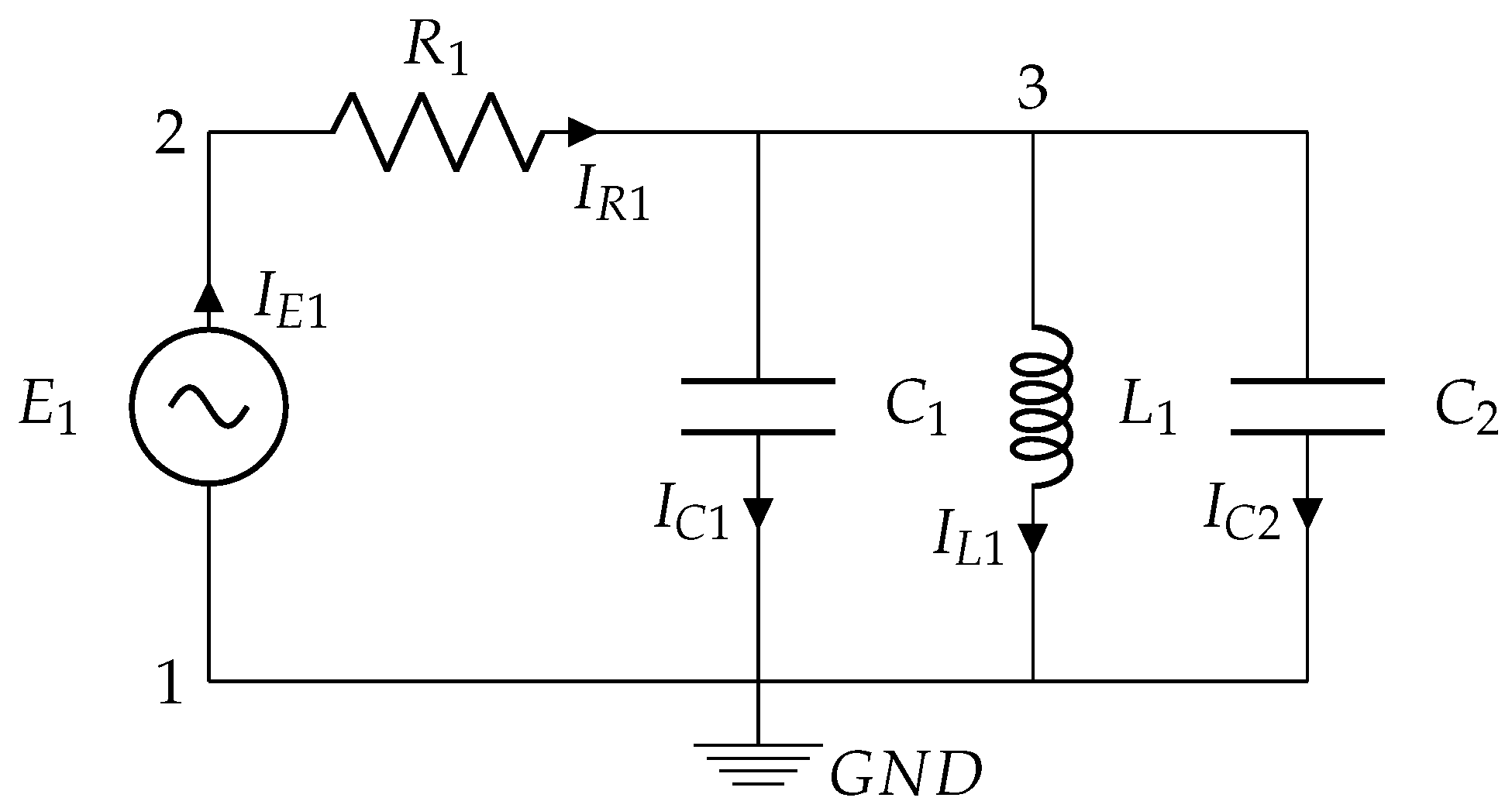
The numerical methods described in Section 2 were evaluated by means of four test problems, which are put forward as benchmarks to evaluate the efficiency and accuracy of time–domain circuit simulations.

3.1. RLC Circuit

The first example is an RLC circuit with constant coefficients and relatively slow dynamics, shown in Figure 1. As is the case with the rest of benchmark examples in this paper, this problem is intended to be easy to replicate and to implement, while providing relevant information about the performance of the methods under study.

Source $E_1$ is defined by the sinusoidal function of time $E_1\left(t\right)=100sin\left(10\pi t\right)$ V. The passive elements in the circuit have constant values $R_1=10\Omega$, $L_1=100$ mH, $C_1=400$ mF, and $C_2=200$ mF. The benchmark simulation consists of a 10-s integration of the system dynamics, for which the initial values of the current through the inductor, $I_{L{1}_0}$, and the voltage of the capacitors, $V_{C{1}_0}$ and $V_{C{2}_0}$, are set to zero.

In this circuit, capacitors $C_1$ and $C_2$ connect nodes 1 and 3 in parallel; their voltages will be related by the two following differential equations:

$$\begin{array}{cc}\hfill & C_1{\dot{V}}_3-C_1{\dot{V}}_1-I_{C1}=0\hfill \end{array}$$

(18)

$$\begin{array}{cc}\hfill & C_2{\dot{V}}_3-C_2{\dot{V}}_1-I_{C2}=0\hfill \end{array}$$

(19)

which are linearly dependent in terms of the system derivatives $\dot{\mathbf{x}}$. This means that matrix $\mathbf{A}$ in Equation (3) is row-rank deficient, which may cause some solvers to fail during the solution of the system dynamics. For instance, the leading matrix in Equation (5) becomes singular, thus preventing most conventional linear solvers from finding a solution for the system derivatives.

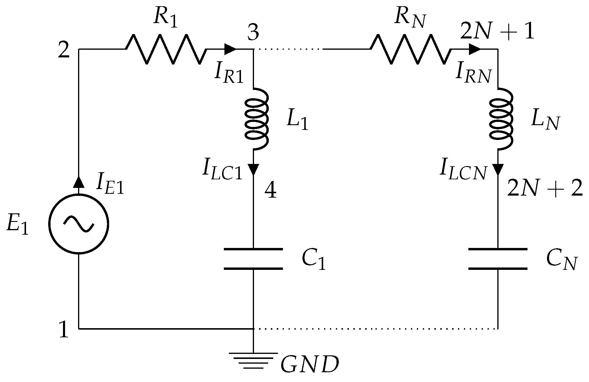
3.2. Scalable RLC Circuit

The second example is a scalable RLC circuit with constant coefficients. The number of system variables can be increased by adding new loops to the circuit, as shown in Figure 2.

Source $E_1$ is the sinusoidal function of time $E_1\left(t\right)=100sin\left(10\pi t\right)$ V. The passive elements in the circuit have the same values in every loop, $R_i=10\Omega$, $L_i=100$ mH and $C_i=100$ mF, where $i=1\dots N$ is the loop number. The benchmark simulation consists of a 1-s integration of the system dynamics, starting from an initial state in which the currents through the inductors, $I_{L{i}_0}$, and the voltage of the capacitors, $V_{C{i}_0}$, are set to zero.

This circuit provides a way to test the computational performance of a method as a function of the problem size, which can be adjusted by selecting a number of loops N. In this work, problems with up to $N=5000$ loops were selected for simulation.

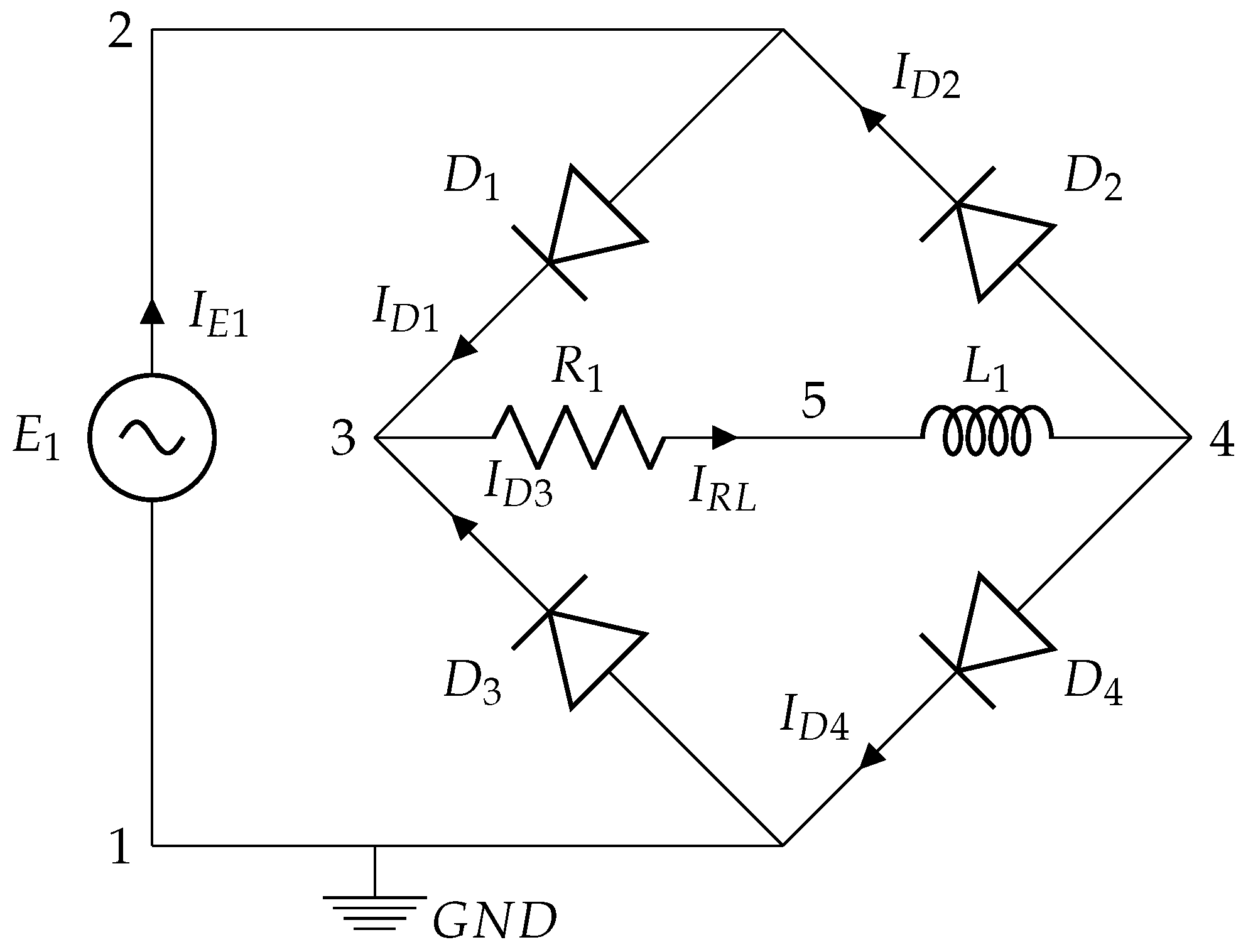
3.3. Full Wave Rectifier

The third example is a model of a full wave rectifier, shown in Figure 3. Source $E_1$ is defined by the sinusoidal function $E_1\left(t\right)=100sin\left(10\pi t\right)$ V. The passive elements in the circuit have constant values $R_1=10\Omega$, and $L_1=100$ mH.

The diodes in this circuit are described using Shockley’s model, shown in Figure 4, and defined by the constitutive equation [30]

$$I-I_{\mathrm{o}}\left(e^{\Delta V/\left(\overline{n}{V}_{\mathrm{t}}\right)}-1\right)=0$$

(20)

where $\Delta V=V_{\mathrm{a}}-V_{\mathrm{c}}$ is the voltage difference between the anode and the cathode of the diode, $I_{\mathrm{o}}=1$ fA is the reverse bias saturation current, $\overline{n}=1.5$ is the ideality factor, and $V_{\mathrm{t}}$ is the thermal voltage defined by

$$V_{\mathrm{t}}=\frac{\overline{k}T}{q}$$

(21)

where q is the electron charge, T is the temperature, and $\overline{k}$ is the Boltzmann constant. The series resistor in Figure 4 has a value of $R_{\mathrm{s}}=1$ mΩ. The benchmark test for this problem consists of a 1-s simulation of the circuit dynamics in which the initial value of the current that flows through the inductor is $I_{R{L}_0}=0$.

This problem is an example of nonlinear electronic circuit with fast changes in the system state during the transitions between the forward and reverse regions of the diodes.

3.4. Synchronous Motor Thermal Equivalent Circuit

The fourth benchmark example is a thermal equivalent circuit to evaluate temperatures and heat flows in a permanent-magnet synchronous motor (PMSM), shown in Figure 5.

Thermal equivalent circuits describe the heat transfer, thermal losses, and thermal inertia properties of a physical system by means of lumped components comparable to those of an electric circuit. Similar models can be found in the literature, e.g., [31,32]. The one presented here aims at balancing the complexity of accurately describing the thermal phenomena that occur in a PMSM and the compactness desirable in a benchmark problem. Each node in the circuit corresponds to a representative point in the physical system and has a certain temperature T associated with it. Heat flows Q between nodes play a role similar to currents in an electric circuit. Thermal conductivity and convection are represented with thermal resistors. Thermal inertia is modelled with capacitors, and heat generation such as Joule effect losses is represented with current sources. The values of thermal resistances, capacitances, and heat sources may be variable if these properties vary as a result of changes in the system temperatures or operation conditions. This is often the case with convective resistors and Joule effect sources.

In the thermal model of the PMSM in Figure 5, all resistances, capacitances, and heat sources are constant, with the exception of the resistance of the air gap between the rotor and the stator ($R_{airgap}$). These parameters are shown in

Table 2. Parameters of the thermal model of the synchronous motor.

Resistor	Value	Capacitor	Value	Loss	Value
	[K/W]		[J/K]		[W]
$R_{axis1}$	1	$C_{axis}$	2000	$Q_{rotor}$	150
$R_{axis2}$	1	$C_{rotor}$	5000	$Q_{copper}$	2000
$R_{innerrotor}$	0.025	$C_{copper}$	2000	$Q_{tooth}$	200
$R_{outerrotor}$	0.015	$C_{stator}$	1500	$Q_{bearing1}$	50
$R_{tooth1}$	0.025	$C_{housing}$	3000	$Q_{bearing2}$	50
$R_{tang}$	0.01	$C_{plate1}$	300
$R_{tooth2}$	0.01	$C_{plate2}$	300
$R_{copper}$	0.001	$C_{bearing1}$	500
$R_{wire}$	0.05	$C_{bearing2}$	500
$R_{yoke}$	0.0025
$R_{housing1}$	0.25
$R_{housing2}$	0.25
$R_{water}$	0.001
$R_{plate1}$	0.5
$R_{plate2}$	0.5
$R_{bearing1}$	3
$R_{housing2}$	3

. The air gap resistance is calculated as a function of the Nusselt number, as detailed in the Appendix A. The benchmark simulation consists of a 5000-s long integration of the system dynamics. The motor is assumed to operate at a constant angular speed $\omega =1570$ rad/s. The temperatures of the cooling fluid and the environment are constant, $T_{water}=320$ K and $T_{env}=300$ K. Initially, the temperature difference between the two nodes connected by a capacitor is zero, which means that the system is at ambient temperature.

This system showcases the characteristics of most thermal equivalent circuits, namely very slow dynamics and physical properties of some components that may vary as the simulation progresses.

3.5. Reference Solutions

Reference solutions are a key component in benchmark problems [24], as they are required to verify the results provided by a certain solver tool, and to compare two or more solutions in terms of accuracy or performance. Analytical closed-form expressions can be obtained for some problems and used as reference solutions. Often, however, these are not available; in such cases, solutions at convergence can be used for the same purpose. These can be found by decreasing the integration tolerances and step-size with which the benchmark problem is solved, until the difference between the obtained results remains below a defined threshold. Solutions at convergence should be obtained with a minimum of two different methods.

In this work, reference solutions were obtained by convergence of two of the DAE solvers described in Section 2.2, namely the ones that used as integrators the trapezoidal rule and the BDF3 formula, decreasing the integration step-size down to 1 μs. Both methods delivered almost identical solutions in all the problems, with a maximum difference in the obtained values of the system variables $\mathbf{x}$ below $2·{10}^{-8}$ A or V in the electric and electronic circuits. For the thermal circuit in Section 3.4, the differences were kept below ${10}^{-8}$ K for the temperatures T, and below $4·{10}^{-3}$ W for the heat flows Q.

For each benchmark problem, a few representative variables (monitored variables) among the n contained in term $\mathbf{x}$ were selected to enable the fast and simple comparison of the simulation results. This set of chosen variables should describe an important behavior aspect of the circuit under study, or critical operational values that need to be kept under control. The total number of variables, algebraic, and differential constraint equations of each benchmark problem is summarized in

Table 3. Number of variables and constraints of proposed benchmark problems.

Problem	Variables	Algebraic ctr.	Differential ctr.
	$\mathit{n}$	$\mathit{m}$	$\mathit{p}$
RLC	8	5	3
Sc. RLC	$3+5N$	$3+3N$	$2N$
Rectifier	20	19	1
Thermal	49	40	9

.

3.5.1. RLC Circuit

The monitored variables in the RLC circuit in Section 3.1 are the voltage at node 3, $V_3$, and the current through the inductor, $I_{L1}$. The reference solutions for these values are shown in Figure 6.

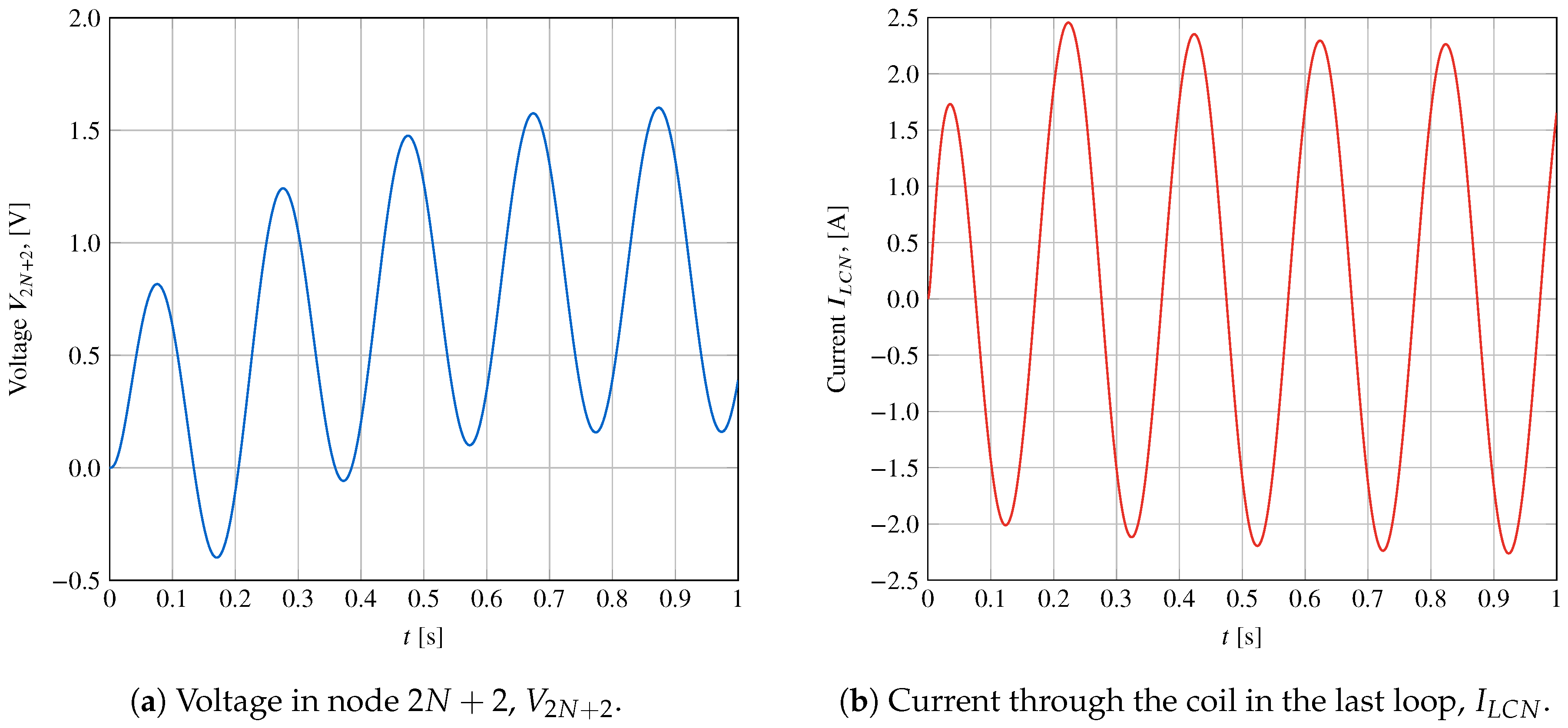
3.5.2. Scalable RLC Circuit

For the scalable RLC circuit in Section 3.2, the monitored variables are the voltage at node $2N+2$ and the current through the last branch in the system, $I_{LCN}$. The time-history of these two variables is shown in Figure 7 for $N=2$ loops.

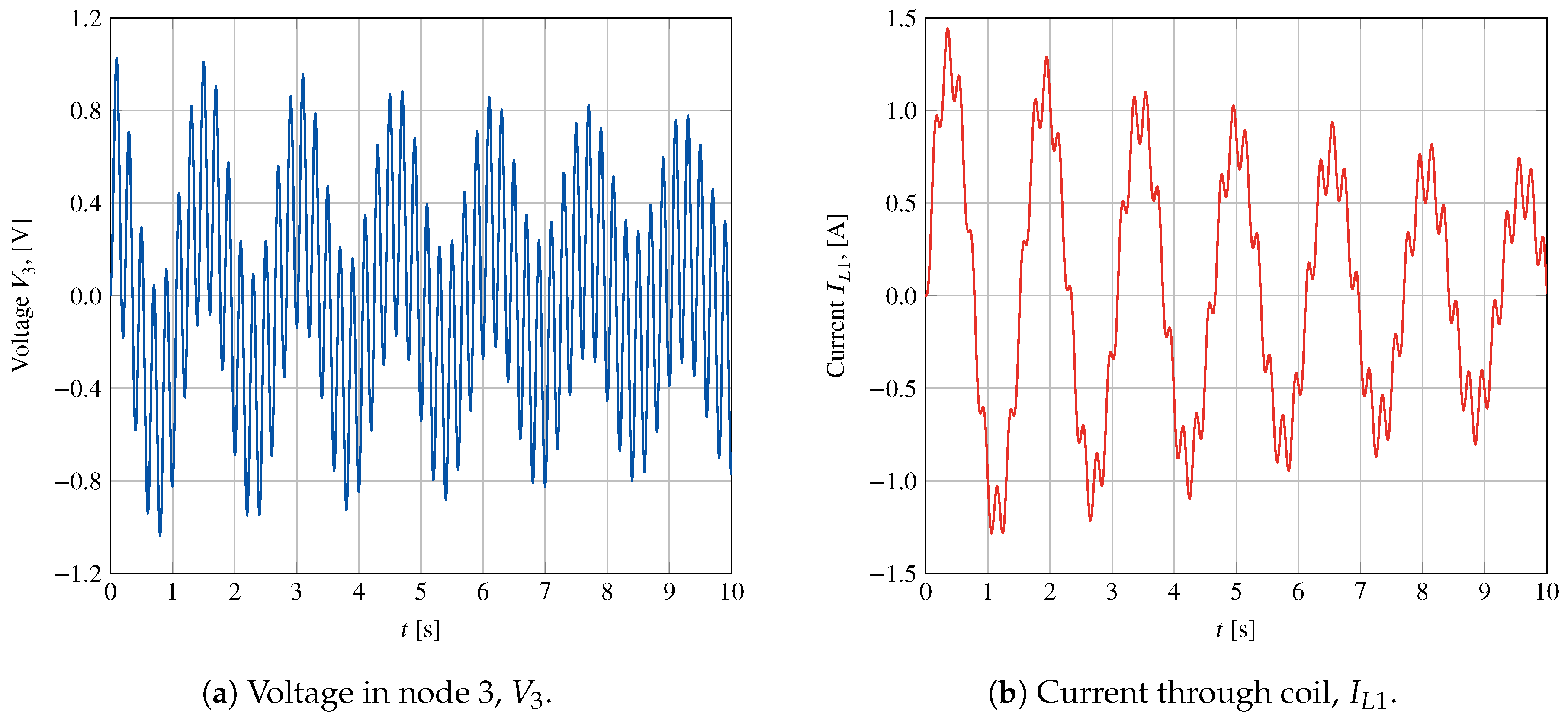
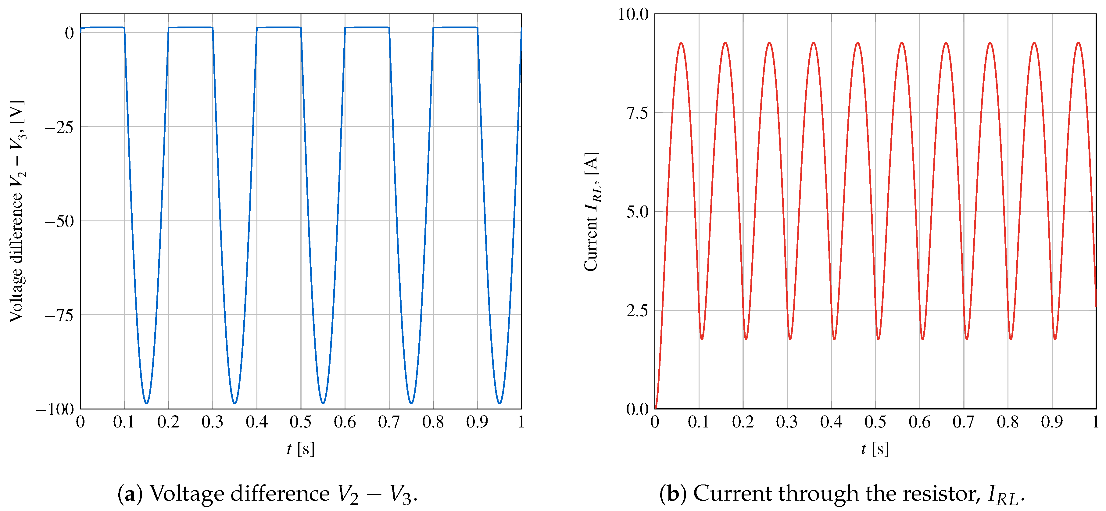
3.5.3. Full Wave Rectifier

For the full wave rectifier in Section 3.3, the monitored variables are the voltage difference between the anode and the cathode of diode 1, $V_2-V_3$, and the current through the resistor and the inductance, $I_{RL}$, shown in Figure 8.

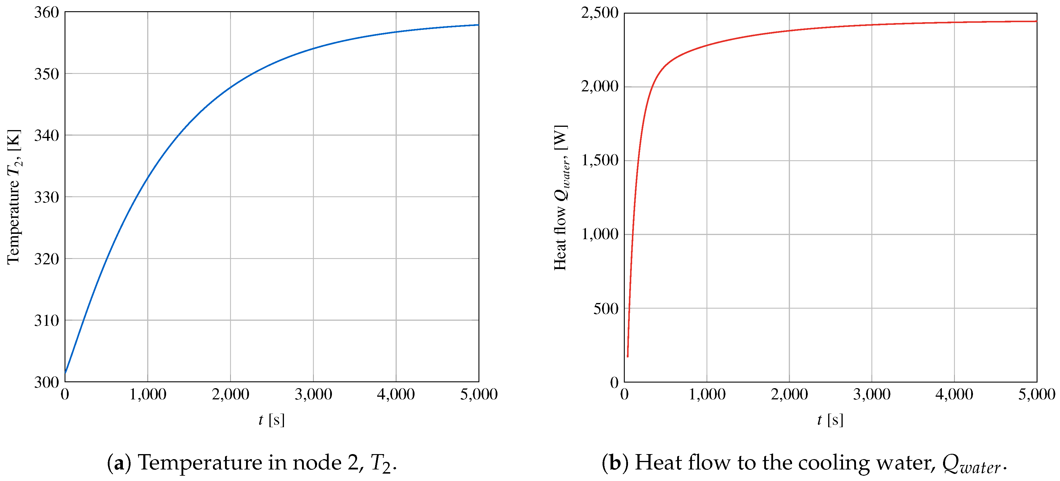
3.5.4. Synchronous Motor

For the thermal circuit of the PMSM, the monitored variables are the temperature of the permanent magnets, $T_2$, and the heat flow from the housing to the refrigerant, $Q_{water}$, which are shown in Figure 9.

3.6. Error Measurement and Performance Evaluation

A main goal of benchmark testing is to determine the performance of a given computational method in the solution of representative problems. For this performance evaluation to be meaningful, comparisons between different methods have to be carried out for the same level of accuracy in the obtained results. This accuracy is measured with respect to the reference solutions discussed in Section 3.5; doing this requires a standard way to evaluate the error of a solution, which is here adapted from [23].

If, for a given point in time $t_{\mathrm{p}}$, $y_{\xi }\left(t_{\mathrm{p}}\right)$ is the solution delivered by a method under study for a variable $\xi$, and $y_{\xi }^{\mathrm{ref}}\left(t_{\mathrm{p}}\right)$ is the reference solution for the same variable, then the error in $\xi$ at time $t_{\mathrm{p}}$ can be defined as

$${\epsilon }_{\xi }\left(t_{\mathrm{p}}\right)=y_{\xi }\left(t_{\mathrm{p}}\right)-y_{\xi }^{\mathrm{ref}}\left(t_{\mathrm{p}}\right).$$

(22)

A number $n_s$ of sampling points equally spaced in time is defined for each benchmark problem. The total error in the simulation for variable $\xi$ is the aggregate

$${\widehat{\epsilon }}_{\xi }=\sqrt{{\displaystyle {\displaystyle \frac{1}{n_s}}\sum _{i=1}^{n_s}{\left({\epsilon }_{\xi }\left(t_i\right)\right)}^2}}.$$

(23)

The number of sampling points $n_s$ for each problem is shown in

Table 4. Simulation length and required number of equally spaced sample points for each benchmark problem.

Circuit	Simulation Time [s]	Sample Points ${\mathit{n}}_{\mathit{s}}$
RLC	10	1000
Sc. RLC	1	100
Rectifier	1	1000
Thermal	5000	5000

.

Two accuracy levels, “low” and “high”, were defined for the simulation of the benchmark examples in this section. These are at least two orders of magnitude larger than the error margins of the reference solutions, pointed out in Section 3.5. Using two accuracy levels helps to determine whether the efficiency properties of a given solution method hold when the precision requirements are made more stringent. A simulation is considered acceptable if the error obtained after the numerical integration process, evaluated with Equation (23), is below the thresholds shown in

Table 5. Acceptable errors in the monitored variables.

Circuit	Precision	Error V or T	Error I or Q
RLC / Sc. RLC	Low	1 mV	1 mA
	High	10 μV	10 μA
Rectifier	Low	1 mV	1 mA
	High	10 μV	10 μA
Thermal	Low	0.1 K	1 W
	High	0.01 K	0.1 W

for every monitored variable.

The comparison of the computational efficiency of two or more simulation methods must be carried out for the same level of accuracy. This criterion was observed in the numerical experiments reported in Section 4.

4. Numerical Experiments

The benchmark problems presented in Section 3 were used to compare the performance and features of the formulations in Section 2. This comparison was carried out taking into consideration the particular requirements of RT simulation. The time invested by the numerical methods in the integration of a time-step must be not only as short as possible, but also predictable. This means that the number of iterations required for the convergence of the Newton iteration to solve Equation (6) must be limited. In principle, the number of iterations could be decreased for those steps that are computationally less challenging, e.g., the intervals between switching points in the rectifier circuit in Section 3.3. This would result in overall shorter computation times. However, most RT applications require that every integration step is solved while meeting RT deadlines. Accordingly, in this work, the number of solver iterations was set to a fixed value, equal for all the integration steps in every method and problem.

The methods in Section 2 were compared in terms of the computation time that was needed to complete the simulation of the benchmark examples within the precision requirements specified in Table 5. Three parameters were adjusted for each method in order to determine its optimal performance in each case: the integration step-size h, the number of solver iterations per time step, $\gamma$, and the integrator tolerance, i.e., its maximum admissible error during iteration, $\epsilon$. Two cases were distinguished when the trapezoidal rule was used as integrator: one in which one projection step was performed upon convergence of the Newton iteration, reported as TR in the following, and another one in which this projection was omitted, labelled TRnP. This makes it possible to determine the impact of the projection step on computation times.

4.1. Simulation Environments

In this research, the use of the benchmark problems and solver implementations was tested under three different computing platforms, namely

• a conventional desktop PC,
• a Beaglebone Black, and
• a Raspberry Pi 4.

The last two environments are ARM-based single-board computers. Testing the benchmark framework and the solver implementations under different software and hardware platforms shows that their application is not restricted to a particular development environment. Moreover, it also serves as a test of the ability of ARM platforms to take on the simulation of particular components in RT computation environments. The features of each simulation environment are summarized in

Table 6. Simulation platform features.

Platform	CPU	Clock Freq.	Cores/	RAM	L1 Cache	L2 Cache	L3 Cache	OS
		[GHz]	Threads	[GB]	[kB]	[MB]	[MB]
PC	Intel i7-8700K	3.7	6/12	8	192/192	1.5	12	Win10
RPi4	ARM A-72	1.5	4/4	4	48/32	1	0	Raspbian 4.19.57
BBB	ARM A-8	1.0	1/1	0.5	32/32	0.25	0	Debian 9.9 IoT

.

Visual Studio 2017 Community was used as compiler under Windows, while gcc-6.3.1 was selected to build the Linux executables for the ARM architectures.

4.2. Numerical Results

The set of solver parameters, $\epsilon$, h, and $\gamma$, was adjusted for each solver and test problem to find out the configuration that delivered the best performance. It was found that decreasing the maximum admissible norm of the residual $\epsilon$ below ${10}^{-3}$ did not result in significant accuracy improvements in any of the examples, and so it was fixed to this value in all the tests. It must be noted that $\widehat{k}$-order BDF methods need a special initialization during their first $\widehat{k}$ steps. These methods use the previous $\widehat{k}$ values of the variables $\mathbf{x}$ to take an integration step; during initialization, these are not available, and so a modified version of the algorithm must be used. In this work, the trapezoidal rule was used as a replacement method for these initial steps. On the other hand, the accuracy requirements for low- and high-precision solutions displayed in Table 5 were enforced in all cases.

4.2.1. RLC Circuit

The direct ODE integration approach in Section 2.1 is unable to perform the simulation of the RLC circuit in Figure 1. Capacitors $C_1$ and $C_2$ connect nodes 1 and 3 in parallel, making the leading matrix $\widehat{\mathbf{A}}$ in Equation (3) rank deficient. Conversely, all the DAE solvers in Section 2.2 were able to complete the integration while attaining the required precision.

Table 7. RLC circuit: Low-precision configuration of the DAE integration methods.

Method	h	$\mathit{\gamma }$	Error V	Error I
	[ms]		[mV]	[mA]
TR	$2.5$	2	$0.25$	$0.38$
BDF1	$2.5·{10}^{-2}$	1	$0.30$	$0.63$
BDF2	$2.5$	2	$0.84$	$0.76$
BDF3	$2.5$	2	$0.14$	$0.33$

and

Table 8. RLC circuit: High-precision configuration of the DAE integration methods.

Method	h	$\mathit{\gamma }$	Error V	Error I
	[ms]		[μV]	[μA]
TR	$0.25$	2	$2.5$	$3.8$
BDF1	$2.5·{10}^{-4}$	1	$3.0$	$6.3$
BDF2	$0.25$	1	$8.4$	$7.6$
BDF3	$0.25$	1	$1.3$	$3.3$

show the selected DAE integrator configurations (step-size h and number of iterations $\gamma$) that resulted in the most efficient solution of the RLC circuit simulation while meeting the low and high precision requirements, respectively. As expected, the errors in the monitored variables scale linearly with the integration step-size h for each method. As shown in Table 8, when BDF integrators are used, decreasing the step-size to achieve high precision makes it possible to reach the desired error levels with a single iteration of the solver. The trapezoidal rule, on the other hand, still required two iterations with the same step-size $h=0.25$ ms.

Table 7 and Table 8 must be interpreted in the light of the results contained in

Table 9. Elapsed times in the simulation of the RLC circuit.

Method	Prec.	Elapsed Time	Elapsed Time	Elapsed Time
		PC [ms]	BBB [ms]	RPi [ms]
TR	Low	$6.5$	$176.8$	$50.6$
TRnP		$3.0$	$92.6$	$34.85$
BDF1		$190.6$	$4988.0$	$815.0$
BDF2		$3.2$	$108.0$	$38.5$
BDF3		$3.4$	$112.8$	$39.6$
TR	High	$69.4$	$1708.1$	$307.0$
TRnP		$32.3$	$856.7$	$162.3$
BDF1		16,764.9	496,852.0	77,287.4
BDF2		$23.3$	$587.8$	$128.6$
BDF3		$24.8$	$636.3$	$133.6$

, which shows the times elapsed in the simulation of the RLC system with each DAE integrator, with the configurations defined in Table 7 and Table 8. Table 9 shows the efficiency delivered by each method for the two accuracy levels, namely high and low, in the solution of the test problem. With the exception of BDF1, all methods would be able to deliver RT performance in the three computing platforms described in Table 6, both for low and high precision. Computations on the BeagleBone Black and the Raspberry Pi 4 were about 30 and 5 times slower than on the PC, respectively. Moreover, results show that the projection stage after convergence of the trapezoidal rule required as much computation time as the convergence of the Newton–Raphson iteration of the main solver. BDF2 and BDF3 delivered the best efficiency in this test problem. It must be mentioned that the tangent in Equation (7) is a constant matrix for this example. This makes it possible to evaluate and factorize it during preprocess; accordingly, only the back-substitution required for the solution of Equation (7) needs to be performed during runtime.

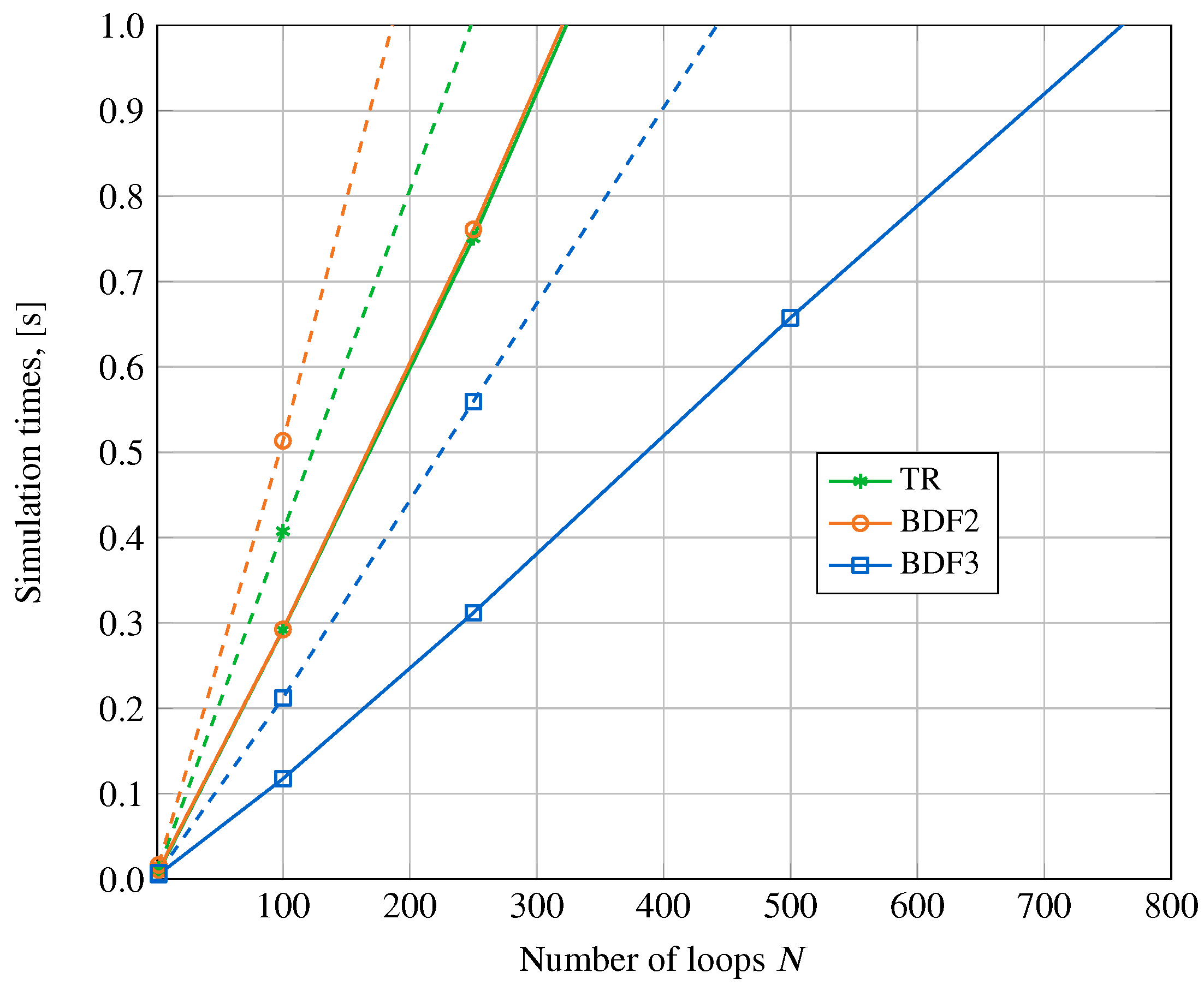
4.2.2. Scalable RLC Circuit

The scalable RLC circuit in Figure 2 was solved using the DAE integration methods in Section 2.2. The integration step-sizes h and number of iterations required by each solver are shown in

Table 10. Scalable RLC circuit ($N=2$ loops): Low-precision configuration of the DAE integration methods.

Method	h	$\mathit{\gamma }$	Error V	Error I
	[ms]		[mV]	[mA]
TR	$2.5$	2	$0.41$	$0.94$
BDF1	$2.5·{10}^{-2}$	1	$0.15$	$0.65$
BDF2	1	2	$0.14$	$0.60$
BDF3	$2.5$	2	$0.38$	$0.54$

and

Table 11. Scalable RLC circuit ($N=2$ loops): High-precision configuration of the DAE integration methods.

Method	h	$\mathit{\gamma }$	Error V	Error I
	[ms]		[μV]	[μA]
TR	$0.25$	2	$4.0$	$9.6$
BDF1	$2.5·{10}^{-4}$	1	$1.5$	$6.5$
BDF2	$0.1$	2	$1.4$	$5.9$
BDF3	$0.25$	2	$3.7$	$2.0$

for low and high precision, respectively.

Table 10 and Table 11 were obtained for a circuit with $N=2$ loops. However, it was verified that these configurations were also able to keep simulation errors with respect to the reference solution below the admissible threshold for circuits with up to $N=5000$ loops. Accordingly, these configurations were used for all the numerical experiments reported in this subsection.

Table 12. Elapsed times in the simulation of the scalable RLC circuit ($N=2$ loops).

Method	Prec.	Elapsed Time	Elapsed Time	Elapsed Time
		PC [ms]	BBB [ms]	RPi [ms]
TR	Low	$0.9$	$32.9$	$10.4$
TRnP		$0.4$	$21.5$	$4.6$
BDF1		$24.0$	$713.3$	$153.7$
BDF2		$1.1$	$40.0$	$12.4$
BDF3		$0.5$	$21.7$	$5.3$
TR	High	$9.8$	$236.6$	$82.8$
TRnP		$3.9$	$116.1$	$37.6$
BDF1		$2191.3$	65,542.3	$9977.6$
BDF2		$10.2$	$337.3$	$74.2$
BDF3		$4.3$	$143.6$	$39.6$

shows the times elapsed by each method in the solution of the RLC circuit with $N=2$ loops. As expected, they feature similar trends to those obtained in Section 4.2.1 with the simple RLC circuit. The tangent matrix in Equation (7) is constant in this problem as well, and so the times in Table 12 do not include its evaluation and factorization.

The simulation of this RLC circuit was repeated varying the number of loops ($N=$ 2, 100, 250, 500, 1000, 2000, 5000) to gain insight into the effect of system size on computational efficiency. These numerical experiments were conducted for both low and high precision. Moreover, an additional set of tests was performed forcing the simulation software to ignore the fact that the tangent matrix is constant and to perform its evaluation and factorization in every solver iteration. Figure 10 and Figure 11 display the elapsed times delivered by each solution approach in the PC simulation platform, for low and high precision, respectively. Elapsed times for the trapezoidal rule (TR) include carrying out the velocity projections. Results for BDF1 were omitted in Figure 11 because the computation times that it required exceeded considerably the ones delivered by the other methods.

Figure 10 and Figure 11 show the computational overhead due to the evaluation and factorization of the tangent matrix. They also show that the increase of elapsed time with the number of loops N (and, as a consequence, with the number of variables n) is approximately linear. This is the result of using sparse matrix implementations and solvers, and agrees with previous results in different simulation domains [29].

The maximum theoretically achievable system sizes that could be simulated while fulfilling RT execution requirements are shown in

Table 13. Scalable RLC circuit: Maximum system size compatible with RT execution on the PC simulation environment.

Method	Precision	Loops	System Size
		[$\mathit{N}$]	[$\mathit{n}$]
TR	Low	2053	10,268
BDF1		48	243
BDF2		1790	8953
BDF3		3661	18,308
TR	High	248	1243
BDF1		-	-
BDF2		186	933
BDF3		447	2238

, for the PC simulation environment. BDF1 experienced convergence issues for large systems in the high-precision simulation, and so results for this method are omitted in this case.

Results in Table 13 include the evaluation and factorization of the tangent matrix. They provide an orientation regarding the maximum system size that the tested methods would be able to handle in a RT simulation environment with the computing power of the PC in Table 6.

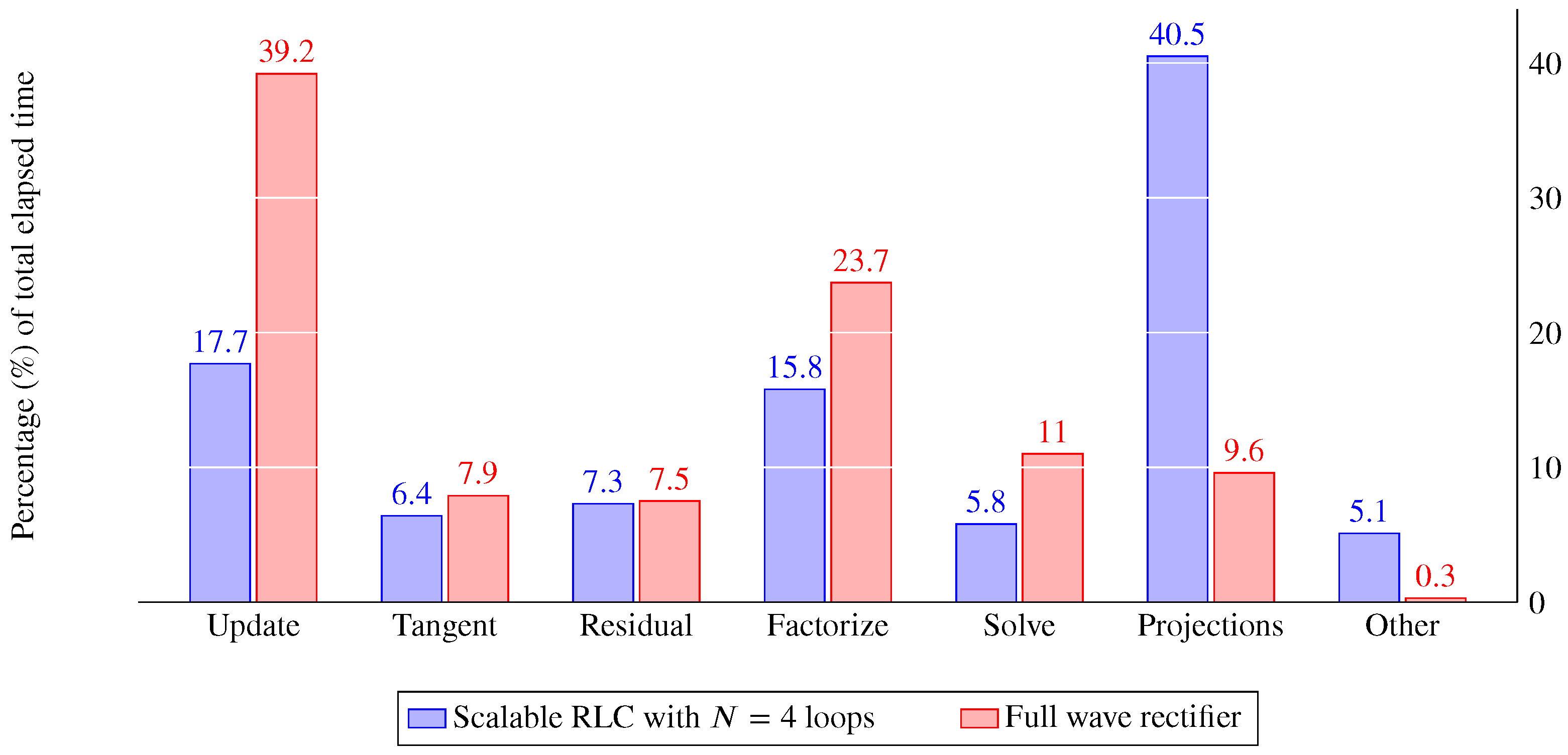
4.2.3. Full Wave Rectifier

The full wave rectifier was solved using the DAE integration methods. The integration step-sizes h and number of iterations required by each integrator are shown in

Table 14. Full wave rectifier: Low-precision configuration of DAE integration methods.

Method	h	$\mathit{\gamma }$	Error V	Error I
	[ms]		[mV]	[mA]
TR	$0.5$	16	$0.17$	$0.29$
BDF1	$0.01$	3	$0.47$	$0.03$
BDF2	$0.25$	7	$0.18$	$0.19$
BDF3	$0.1$	9	$4.0·{10}^{-3}$	$7.9·{10}^{-3}$

and

Table 15. Full wave rectifier: High-precision configuration of DAE integration methods.

Method	h	$\mathit{\gamma }$	Error V	Error I
	[ms]		[μV]	[μA]
TR	$0.05$	6	$2.0$	$1.8$
BDF1	${10}^{-4}$	1	$4.7$	$0.3$
BDF2	$0.05$	9	$7.9$	$6.5$
BDF3	$0.1$	9	$4.0$	$7.9$

for low and high precision, respectively.

Table 16. Elapsed times in the simulation of the full wave rectifier circuit.

Method	Prec.	Elapsed Time	Elapsed Time	Elapsed Time
		PC [ms]	BBB [ms]	RPi [ms]
TR	Low	$47.0$	$1103.8$	$223.5$
TRnP		$42.7$	$984.0$	$220.3$
BDF1		$391.4$	$9821.6$	$1719.3$
BDF2		$37.8$	$924.1$	$223.5$
BDF3		$125.1$	$3025.8$	$574.2$
TR	High	$206.3$	$4817.1$	$913.8$
TRnP		$161.2$	$3805.3$	$724.9$
BDF1		14,009.5	141,564.0	61,429.0
BDF2		$241.6$	$5897.7$	$1060.0$
BDF3		$125.1$	$3025.8$	$574.2$

contains the elapsed times for each method and error criterion.

Unlike the RLC examples, the rectifier is a nonlinear problem with relatively fast changes in its dynamics. Each diode in this system can be in a reverse or forward state; iterative solvers may run into numerical issues during the transitions between them. Moreover, the tangent matrix of the system is not constant and has to be evaluated and factorized at every solver iteration. This explains the comparatively longer computation times and higher number of iterations required for convergence in this example. The abruptly changing dynamics of the rectifier results in the need to use integration steps smaller than $h=0.1$ ms with the BDF3 solver, even for low precision requirements. Increasing the step-size beyond this limit causes the errors with respect to the reference solution to rise quickly and, eventually, leads to the failure of the simulation. This fact points towards the difficulty that high-order multi-step integrators experience to keep the simulation of discontinuous systems stable. When low precision results are acceptable, TR and BDF2 are preferable in terms of efficiency, as confirmed by the results in Table 16.

The full wave rectifier example can also be used to highlight the importance of keeping the derivative-level violation of algebraic constraints under control when using certain integrators. Figure 12 shows the derivative with respect to time of the voltage at node 5, ${\dot{V}}_5$, obtained with three different integration approaches, namely BDF3 and the trapezoidal rule (TR) with and without the projection step in Equation (16). As expected, BDF3 and the projected TR deliver the same results. The uncorrected TR, however, delivers a magnitude of ${\dot{V}}_5$ that consistently increases with time. It must be stressed that the three simulations used to obtain Figure 12 satisfied the algebraic constraints $\mathsf{\Phi }=\mathbf{0}$ and the differential equations $\mathbf{A}\dot{\mathbf{x}}+\mathbf{b}=\mathbf{0}$, explicitly imposed by Equation (8). Accordingly, they obtain very similar values of the system variables $\mathbf{x}$, within the acceptable values in Table 5. This is not the case with the derivatives with respect to time $\dot{\mathsf{\Phi }}={\mathsf{\Phi }}_{\mathbf{x}}\dot{\mathbf{x}}+{\mathsf{\Phi }}_t=\mathbf{0}$. The TR integration formula is compatible with the accumulation of derivative-level errors, as long as the obtained values of $\dot{\mathbf{x}}$ satisfy the differential equations of the circuit. The BDF3 method suffers from the same limitation, but it does not reuse the derivatives to evaluate future values of $\dot{\mathbf{x}}$.

As shown in Figure 12 and Figure 13, the projection step removes the accumulation of derivative-level constraint violations and prevents $\dot{\mathbf{x}}$ from reaching excessive values that could eventually lead to numerical errors in the computations or even to the simulation failure by overflow.

Figure 14 shows the distribution of computational workload between the different tasks during a time-step for the full wave rectifier, solved with low precision requirements. The trapezoidal rule was used as integrator. Results are compared to those delivered by the scalable RLC circuit with $N=4$ loops, which is similar to the rectifier in terms of system size. The solver was forced to repeat the evaluation and factorization of the tangent matrix in each solver iteration in both examples. The integration step can be divided into the following tasks:

• the update of the dynamic terms $\mathsf{\Phi }$, $\mathbf{A}$, $\mathbf{b}$, and their derivatives;
• the evaluation of the residual $\mathbf{f}$ and the tangent matrix $\mathrm{d}\mathbf{f}/\mathrm{d}\mathbf{x}$ in Equation (7);
• the factorization and backsubstitution of the linear solver in Equation (7);
• the projections in Equation (16); and
• other operations, such as the update of variables and regulation of code execution.

The profiling results confirmed that the computational effort of the projection step amounts to two or three iterations of the main system solver for the studied systems. For circuits that require a considerable number of solver iterations, such as the rectifier, the overhead of the projection step is less relevant in relative terms than it would be in RLC systems, where convergence is achieved with one or two iterations.

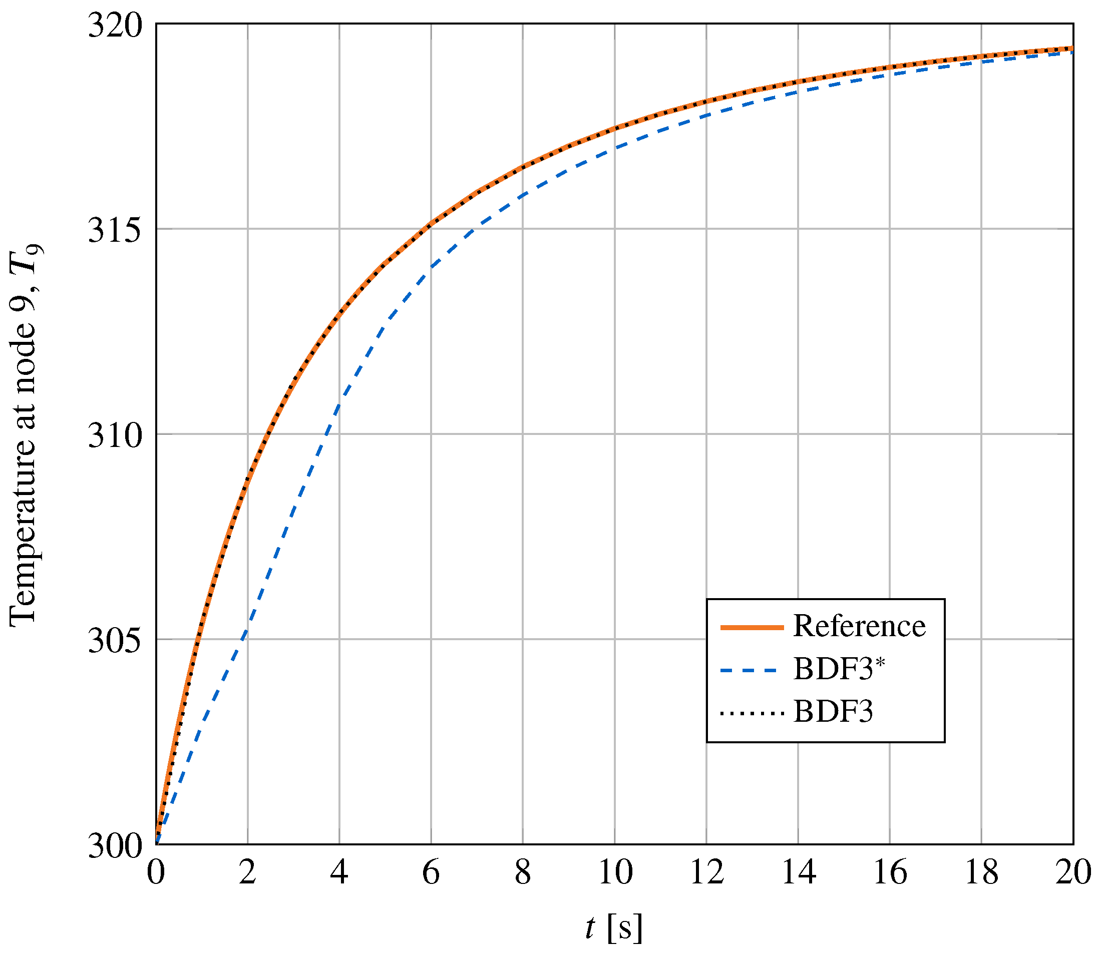
4.2.4. Synchronous Motor

The thermal equivalent circuit that corresponds to the synchronous motor was also solved using the DAE integration methods. The step-sizes h and number of iterations per step are shown in

Table 17. Synchronous motor: Low-precision configuration of the DAE integration methods.

Method	h	$\mathit{\gamma }$	Error T	Error Q
	[ms]		[K]	[W]
TR	500	2	$9.36·{10}^{-7}$	$0.612$
BDF1	25	2	$1.49·{10}^{-4}$	$0.839$
BDF2	250	2	$9.01·{10}^{-7}$	$0.523$
BDF3	500	2	$3.12·{10}^{-7}$	$0.388$

and

Table 18. Synchronous motor: High-precision configuration of the DAE integration methods.

Method	h	$\mathit{\gamma }$	Error T	Error Q
	[ms]		[K]	[W]
TR	100	2	$6.03·{10}^{-8}$	$0.024$
BDF1	$2.5$	2	$1.49·{10}^{-5}$	$0.085$
BDF2	100	2	$1.56·{10}^{-7}$	$0.092$
BDF3	250	2	$6.54·{10}^{-8}$	$0.060$

for low and high precision, respectively.

Table 17 and Table 18 show that the order of magnitude of the error in heat flows is much larger than that of the error in temperatures; the accuracy in the calculation of the heat flows becomes thus more critical to determine if a simulation is correct or not.

Table 19. Elapsed times in the simulation of the thermal circuit of the synchronous motor.

Method	Prec.	Elapsed Time	Elapsed Time	Elapsed Time
		PC [s]	BBB [s]	RPi [s]
TR	Low	$0.12$	$2.81$	$0.59$
TRnP		$0.06$	$1.28$	$0.27$
BDF1		$1.12$	$26.29$	$5.79$
BDF2		$0.12$	$2.86$	$0.58$
BDF3		$0.06$	$1.60$	$0.32$
TR	High	$0.55$	$14.03$	$2.82$
TRnP		$0.27$	$6.34$	$1.40$
BDF1		$10.88$	$264.15$	$56.08$
BDF2		$0.29$	$7.17$	$1.49$
BDF3		$0.12$	$3.20$	$0.64$

contains the elapsed times for every configuration and integration method. All methods are well below the real-time limit in all cases, regardless of the selected computation environment.

Besides having slower dynamics and time-varying properties, thermal equivalent circuits differ from their conventional RC counterparts in that they are often subjected to excitations that are not periodic. The system behavior during transients is a relevant part of the dynamics and needs to be determined accurately in most applications. The initialization method plays an important role in the evaluation of the first transient in the simulation; unsuitable initialization approaches result in incorrect predictions during the first integration steps that affect negatively the simulation accuracy long after the initialization phase is complete.

Figure 15 shows that the temperature $T_9$ delivered by the BDF3 integrator using the TR as initialization routine (BDF3) matches the reference solution, even with an integration step-size $h=1$ s. On the other hand, if the initialization is not properly performed, for instance assuming a constant value of the temperature before $t=0$ (BDF3${}^{*}$), the effect of initialization errors can be appreciated much later in the simulation, rendering it visibly inaccurate. This behavior was not observed in the electric and electronic circuits in Section 3.1, Section 3.2 and Section 3.3, in which errors derived from poor initialization approaches were quickly corrected upon completion of the initial transient.

5. Conclusions

This paper puts forward a methodology to evaluate the performance of time–domain simulation methods for electric, electronic, and thermal equivalent circuits, oriented towards the determination of their suitability to be used in real-time environments. Four benchmark problems with their corresponding reference solutions were defined, together with error metrics and accuracy criteria to enable the comparison of different methods. These examples are easy to reproduce and representative of significant problem types in circuit simulation.

The proposed methodology was used to assess the capability of ODE and DAE solver methods to deliver RT performance in three different hardware and software environments, including ARM boards with limited computing capabilities. The tested methods included transforming the circuit equations into a system of ODEs prior to their numerical integration, and Newton–Raphson iterative solvers for nonlinear systems of DAEs. Backward difference methods and the trapezoidal rule were used as integration formulas.

The numerical experiments performed in this study demonstrated that the benchmarking methodology and the examples can be used to obtain relevant information regarding the performance and features of a given solution method. Results made it possible to discard the direct ODE integration as a generally valid approach, at least in the form presented in the methods section in this paper. Among the DAE solver methods, the first-order BDF integrator, BDF1, consistently showed low performance, requiring very small integration step-sizes, down to three orders of magnitude smaller than those required by the other formulas, to attain the accuracy requirements defined in the benchmark. This rendered it unsuitable except for the simulation of the simplest test cases.

Implementations based on second and third order BDF formulas and the trapezoidal rule delivered comparable performances. For systems with relatively slow dynamics, BDF3 always delivered the best efficiency. TR and BDF2, on the other hand, could be used to obtain faster computations in circuits with nonsmooth behavior when the level of accuracy can be relaxed. A proper initialization of BDF methods is required to obtain accurate simulation results, especially in circuits in which the excitation is not periodic.

Regarding the RT ability of the tested methods, the benchmark framework can be used to provide orientations regarding the scope of applicability of a method in a certain computing platform. With the PC used in this study, BDF2, BDF3, and TR were able to solve all the problems in the benchmark below the RT mark. For RLC circuits, systems of up to a few thousand variables, depending on the requested precision, could be integrated below this limit. Results also show that ARM single-board computers can also be used to simulate most problems in the benchmark set. However, more factors than computational efficiency determine the usability of a method in RT computing, such as system latency and communication delays. The results from benchmarking can be used to rule out inefficient or inadequate approaches, and to choose the most effective options when dealing with the solution of a given problem.

Besides conclusions about efficiency, the simulation of the benchmark problems led to the identification of issues with the evaluation of the derivatives with respect to time of the system variables. Integration methods that determine the derivatives in future steps using previously computed values of the same derivatives need to enforce the satisfaction of the derivatives with respect to time of the algebraic equations of the circuit. Failure to do so may result in the accumulation of errors in the system derivatives, which can eventually lead to numerical issues in problem solutions. The trapezoidal rule is one of these methods; a projection step was introduced in this paper to address this need of the integrator. It was observed that the computational requirements of the projection step are comparable to those of two or three iterations of the DAE solver.

References

1. Pastorino, R.; Cosco, F.; Naets, F.; Desmet, W.; Cuadrado, J. Hard real-time multibody simulations using ARM-based embedded systems. Multibody Syst. Dyn. 2016, 37, 127–143. [Google Scholar] [CrossRef]
2. Andersson, H.; Nordin, P.; Borrvall, T.; Simonsson, K.; Hilding, D.; Schill, M.; Krus, P.; Leidermark, D. A co-simulation method for system-level simulation of fluid–structure couplings in hydraulic percussion units. Eng. Comput. 2017, 33, 317–333. [Google Scholar] [CrossRef] [Green Version]
3. Nguyen, V.; Besanger, Y.; Tran, Q.; Nguyen, T. On conceptual structuration and coupling methods of co-simulation frameworks in cyber-physical energy system validation. Energies 2017, 10, 1977. [Google Scholar] [CrossRef] [Green Version]
4. Gomes, C.; Thule, C.; Broman, D.; Larsen, P.G.; Vangheluwe, H. Co-simulation: A survey. ACM Comput. Surv. 2018, 51, 49:1–49:33. [Google Scholar] [CrossRef]
5. Sadjina, S.; Pedersen, E. Energy conservation and coupling error reduction in non-iterative co-simulations. Eng. Comput. 2019. [Google Scholar] [CrossRef] [Green Version]
6. Rodríguez, B.; González, F.; Naya, M.A.; Cuadrado, J. A test framework for the co-simulation of electric powertrains and vehicle dynamics. In Proceedings of the ECCOMAS Thematic Conference on Multibody Dynamics, Duisburg, Germany, 15–18 July 2019. [Google Scholar]
7. Stettinger, G.; Benedikt, M.; Tranninger, M.; Horn, M.; Zehetner, J. Recursive FIR-filter design for fault-tolerant real-time co-simulation. In Proceedings of the 2017 25th Mediterranean Conference on Control and Automation (MED), Valletta, Malta, 3–6 July 2017. [Google Scholar] [CrossRef]
8. Rahikainen, J.; González, F.; Naya, M.Á. An automated methodology to select functional co-simulation configurations. Multibody Syst. Dyn. 2020, 48, 79–103. [Google Scholar] [CrossRef] [Green Version]
9. Nagel, L.W.; Pederson, D.O. Simulation program with integrated circuit emphasis. In Proceedings of the sixteenth Midwest Symposium on Circuit Theory, Waterloo, ON, Canada, 12 April 1973. [Google Scholar]
10. Chua, L.O.; Li, P.M. Computer-Aided Analysis of Electronic Circuits; Prentice-Hall: Englewood Cliffs, NJ, USA, 1975. [Google Scholar]
11. Newmark, N.M. A method of computation for structural dynamics. J. Eng. Mech. Div. ASCE 1959, 85, 67–94. [Google Scholar]
12. Hairer, E.; Nørsett, S.P.; Wanner, G. Solving Ordinary Differential Equations I; Springer: Berlin, Germany, 1993. [Google Scholar] [CrossRef] [Green Version]
13. Fijnvandraat, J.G.; Houben, S.H.M.J.; ter Maten, E.J.W.; Peters, J.M.F. Time domain analog circuit simulation. J. Comput. Appl. Math. 2006, 185, 441–459. [Google Scholar] [CrossRef] [Green Version]
14. Maffezzoni, P.; Codecasa, L.; D’Amore, D. Time-domain simulation of nonlinear circuits through implicit Runge-Kutta methods. IEEE Trans. Circuits Syst. I Regul. Pap. 2007, 54, 391–400. [Google Scholar] [CrossRef]
15. Yuan, F.; Opal, A. Computer methods for switched circuits. IEEE Trans. Circuits Syst. I Fundam. Theory Appl. 2003, 50, 1013–1024. [Google Scholar] [CrossRef]
16. Acary, V.; Bonnefon, O.; Brogliato, B. Time-stepping numerical simulation of switched circuits within the nonsmooth dynamical systems approach. IEEE Trans. Comput.-Aided Des. Integr. Circuits Syst. 2010, 29, 1042–1055. [Google Scholar] [CrossRef]
17. Ebert, F.; Bächle, S. Element-based index reduction in electrical circuit simulation. PAMM 2006, 6, 731–732. [Google Scholar] [CrossRef]
18. Steinbrecher, A.; Stykel, T. Model Order Reduction of Electrical Circuits with Nonlinear Elements. In Progress in Industrial Mathematics at ECMI 2010; Springer: Berlin/Heidelberg, Germany, 2012; pp. 169–177. [Google Scholar] [CrossRef]
19. Davoudi, A.; Jatskevich, J.; Chapman, P.L.; Bidram, A. Multi-resolution modeling of power electronics circuits using model-order reduction techniques. IEEE Trans. Circuits Syst. I Regul. Pap. 2013, 60, 810–823. [Google Scholar] [CrossRef]
20. Dufour, C.; Abourida, S.; Bélanger, J. Real-time simulation of electrical vehicle motor drives on a PC cluster. In Proceedings of the 10th European Conference on Power Electronics and Applications (EPE-2003), Toulouse, France, 2–4 September 2003. [Google Scholar]
21. Almaguer, J.; Cárdenas, V.; Espinoza, J.; Aganza-Torres, A.; González, M. Performance and control strategy of real-time simulation of a three-phase solid-state transformer. Appl. Sci. 2019, 9, 789. [Google Scholar] [CrossRef] [Green Version]
22. Zhang, B.; Jin, X.; Tu, S.; Jin, Z.; Zhang, J. A new FPGA-based real-time digital solver for power system simulation. Energies 2019, 12, 4666. [Google Scholar] [CrossRef] [Green Version]
23. González, M.; Dopico, D.; Lugrís, U.; Cuadrado, J. A benchmarking system for MBS simulation software: Problem standardization and performance measurement. Multibody Syst. Dyn. 2006, 16, 179–190. [Google Scholar] [CrossRef]
24. González, M.; González, F.; Luaces, A.; Cuadrado, J. A collaborative benchmarking framework for multibody system dynamics. Eng. Comput. 2010, 26, 1–9. [Google Scholar] [CrossRef]
25. Hu, Z.; Du, M.; Wei, K.; Hurley, W.G. An adaptive thermal equivalent circuit model for estimating the junction temperature of IGBTs. IEEE J. Emerg. Sel. Top. Power Electron. 2019, 7, 392–403. [Google Scholar] [CrossRef]
26. Bayo, E.; Ledesma, R. Augmented Lagrangian and mass–orthogonal projection methods for constrained multibody dynamics. Nonlinear Dyn. 1996, 9, 113–130. [Google Scholar] [CrossRef]
27. Dopico, D.; González, F.; Cuadrado, J.; Kövecses, J. Determination of holonomic and nonholonomic constraint reactions in an index-3 augmented Lagrangian formulation with velocity and acceleration projections. J. Comput. Nonlinear Dyn. 2014, 9. [Google Scholar] [CrossRef]
28. Davis, T.A.; Natarajan, E.P. Algorithm 907: KLU, a direct sparse solver for circuit simulation problems. ACM Trans. Math. Softw. 2010, 37, 1–17. [Google Scholar] [CrossRef]
29. González, M.; González, F.; Dopico, D.; Luaces, A. On the effect of linear algebra implementations in real-time multibody system dynamics. Comput. Mech. 2008, 41, 607–615. [Google Scholar] [CrossRef]
30. Sah, C.; Noyce, R.; Shockley, W. Carrier generation and recombination in P-N junctions and P-N junction characteristics. Proc. IRE 1957, 45, 1228–1243. [Google Scholar] [CrossRef]
31. Touhami, S.; Bertin, Y.; Lefèvre, Y.; Llibre, J.F.; Henaux, C.; Fénot, M. Lumped Parameter Thermal Model of Permanent Magnet Synchronous Machines; Technical Report; LAPLACE-LAboratoire PLasma et Conversion d’Energie: Toulouse, France, 2017. [Google Scholar]
32. Chen, Q.; Zou, Z.; Cao, B. Lumped-parameter thermal network model and experimental research of interior PMSM for electric vehicle. CES Trans. Electr. Mach. Syst. 2017, 1, 367–374. [Google Scholar] [CrossRef]
33. Incropera, F.P.; Dewitt, D.P.; Bergman, T.L.; Lavine, A.S. Fundamentals of Heat and Mass Transfer; John Wiley & Sons: Hoboken, NJ, USA, 2007. [Google Scholar]
Figure 1. Diagram of an RLC circuit with constant coefficients.
Energies 13 01354 g001
Figure 2. Diagram of a scalable RLC circuit with constant coefficients.
Energies 13 01354 g002
Figure 3. Model of a full wave rectifier.
Energies 13 01354 g003
Figure 4. Diode model used in the full wave rectifier.
Energies 13 01354 g004
Figure 5. Thermal model of a permanent-magnet synchronous motor.
Energies 13 01354 g005
Figure 6. Reference solutions for RLC circuit.
Energies 13 01354 g006
Figure 7. Reference solutions for the scalable RLC circuit, with N = 2.
Energies 13 01354 g007
Figure 8. Reference solutions for the full wave rectifier.
Energies 13 01354 g008
Figure 9. Reference solutions for the synchronous motor.
Energies 13 01354 g009
Figure 10. Scalable RLC circuit: Simulation time as a function of the number of loops (N) for low precision. Simulations with a constant tangent matrix are represented with solid lines; dashed lines mean refactorization of the tangent matrix in each solver iteration.
Energies 13 01354 g010
Figure 11. Scalable RLC circuit: Simulation time as a function of the number of loops (N) for high precision. Simulations with a constant tangent matrix are represented with solid lines; dashed lines mean refactorization of the tangent matrix in each solver iteration.
Energies 13 01354 g011
Figure 12. Full wave rectifier: Derivative with respect to time of the voltage at node 5, V ˙ 5 .
Energies 13 01354 g012
Figure 13. Full wave rectifier: Norm of derivative-level constraint violations term, Φ ˙ .
Energies 13 01354 g013
Figure 14. Percentage of total runtime elapsed by the TR method in each stage of the time-step.
Energies 13 01354 g014
Figure 15. Synchronous motor: First, 20 s of the time history of the temperature at node 9, T 9 , obtained with h = 1 s.
Energies 13 01354 g015