Qualitative and Quantitative Transient Stability Assessment of Stand-Alone Hybrid Microgrids in a Cluster Environment


Abstract
1. Introduction
- Detailed dynamic modelling of classical and hybrid microgrids—representing four hybrid scenarios with respect to different points in time on a summer day—comprising DGs, grid-feeding PV, grid-forming BSS, as well as static and dynamic loads in a cluster environment.
- Comparison of critical clearing time (CCT) profiles of the microgrids with respect to the four hybrid scenarios and the classical scenario (with DGs only) as well as three operating modes, namely island, interconnection, and cluster mode.
- Qualitative stability assessment by comparing the behavior of the four hybrid microgrids (i.e., hybrid scenarios in cluster mode) with that of the classical microgrid for a three-phase short-circuit location.
- Qualitative investigation of the impact of different degrees of coupling (i.e., operating modes) of microgrids on the system stability.
- Quantitative TSA using the micro-hybrid method in the scenarios and operating modes by investigating the system stability degree with respect to different clearing times for the same fault location.
- Quantitative analysis of the critical energy and of the effect of the fault location on the critical energy in the cluster mode.
2. Methodology
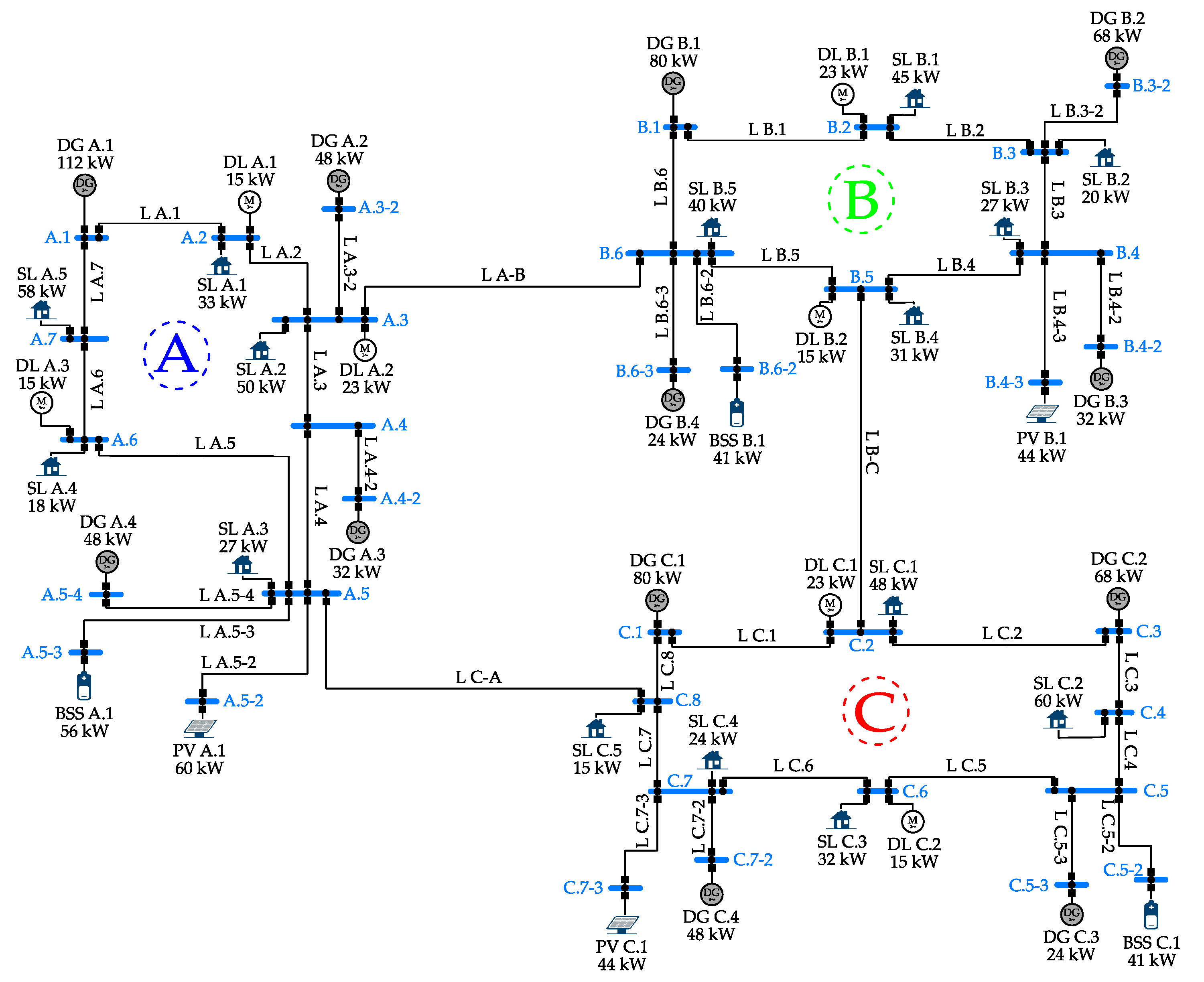
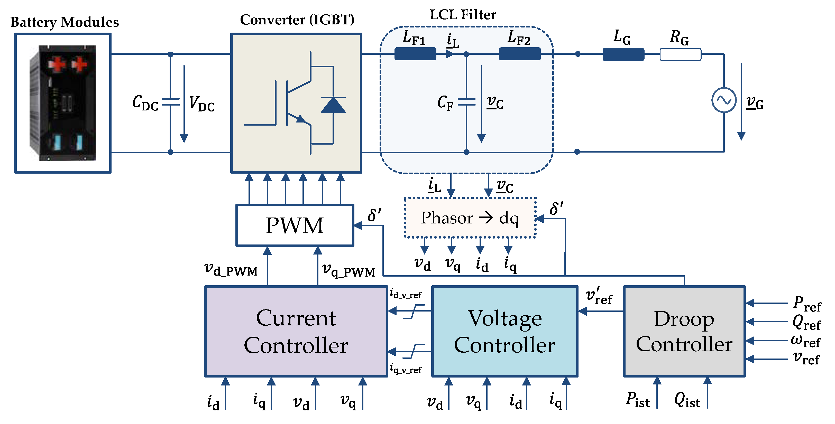
2.1. System Modelling
- High mechanical (engine) loading of DGs (70%–80%)
- High PV feed-in (75%–85% of the nominal real power)
- High consumption/feed-in of BSS (60%–90% of the nominal real power)
- Allowable maximum and minimum voltage and frequency values according to the international norm ISO 8528-5 in the steady-state and sudden load change.
2.2. Overview of Scenarios and Operating Modes
2.3. Dimensioning of Controllers in Photovoltaics and Battery Storage Systems
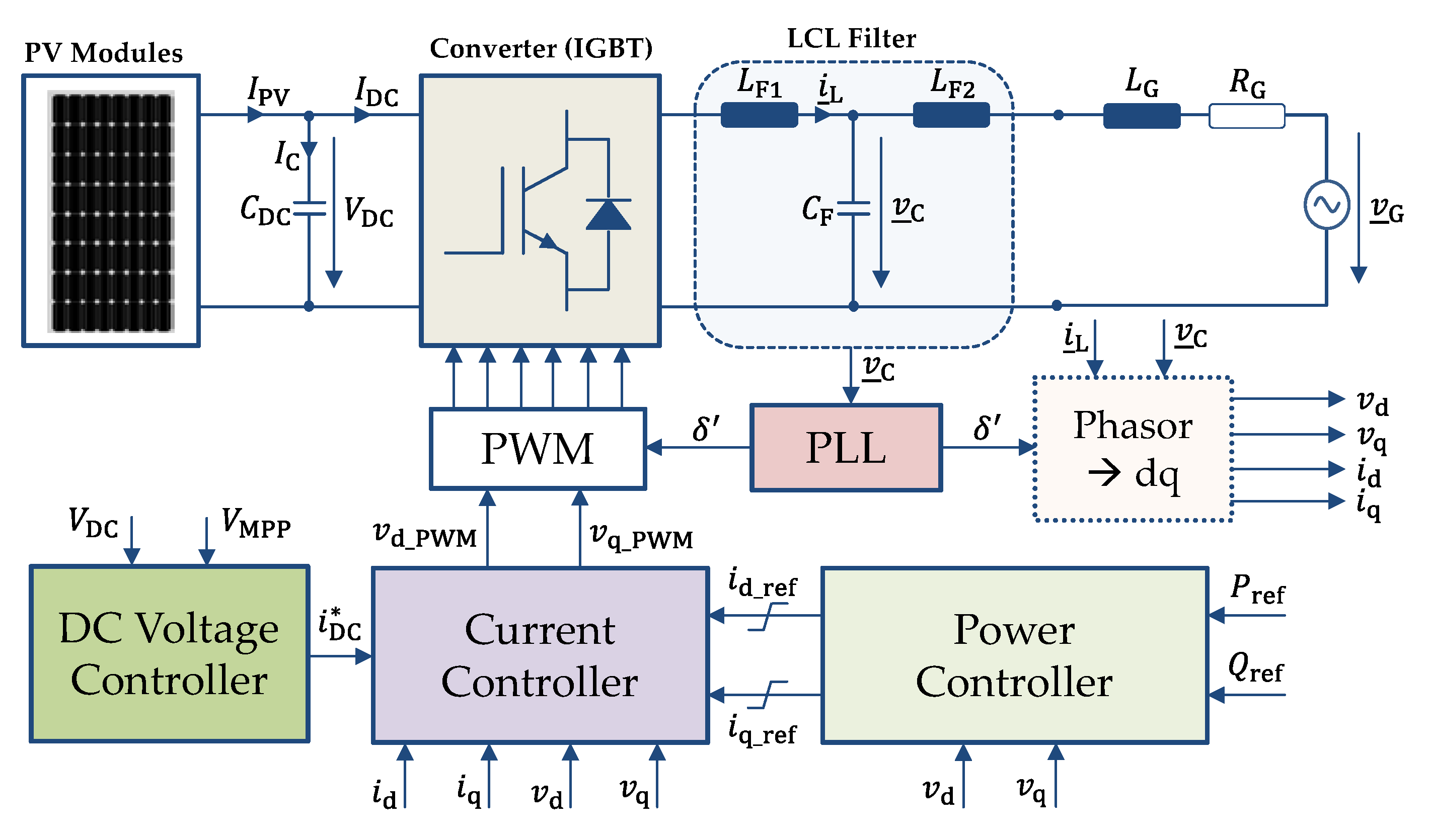
2.3.1. Photovoltaics
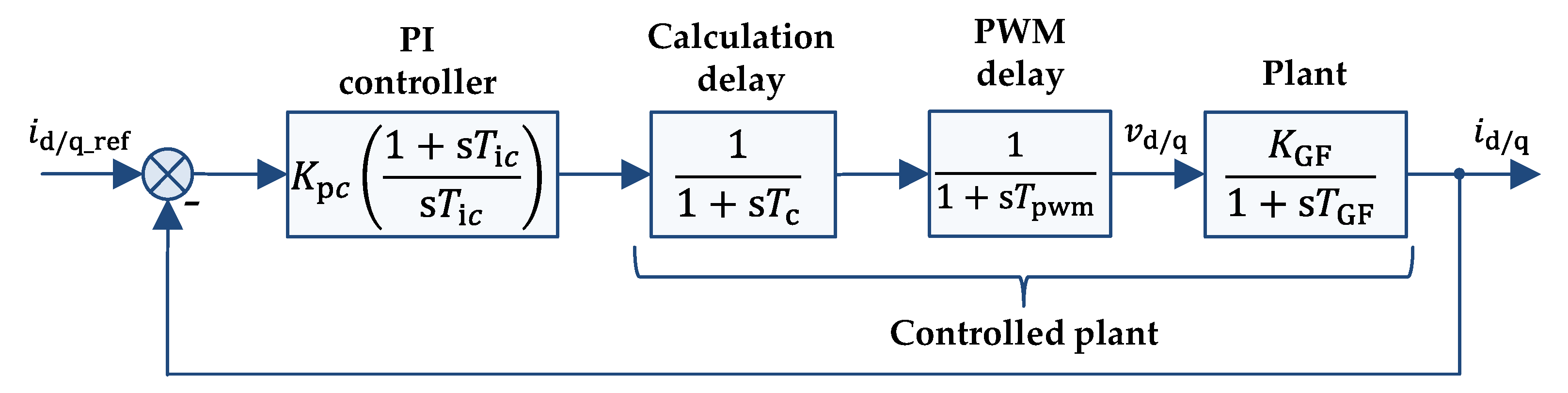
Current Controller
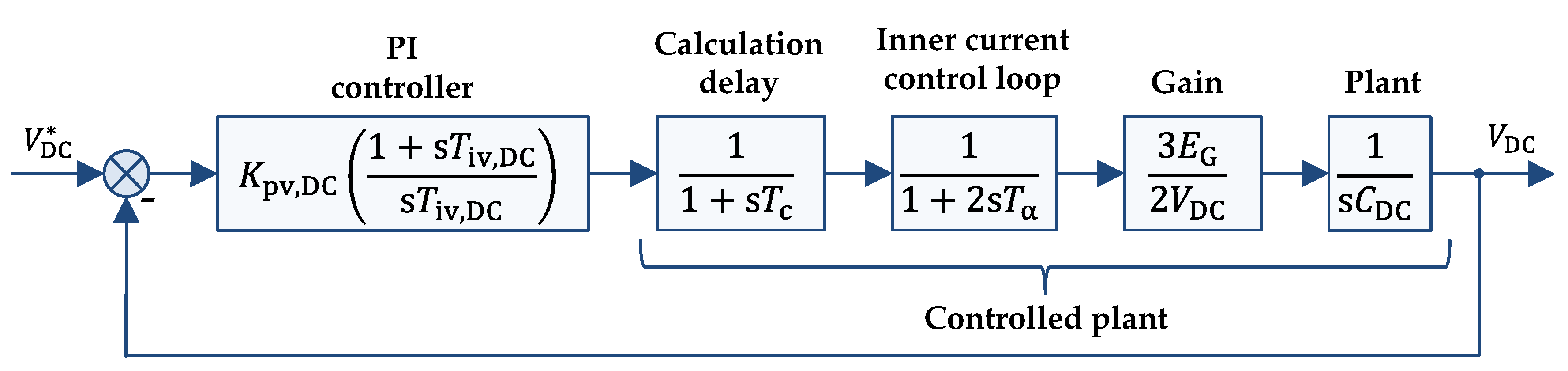
DC Voltage Controller
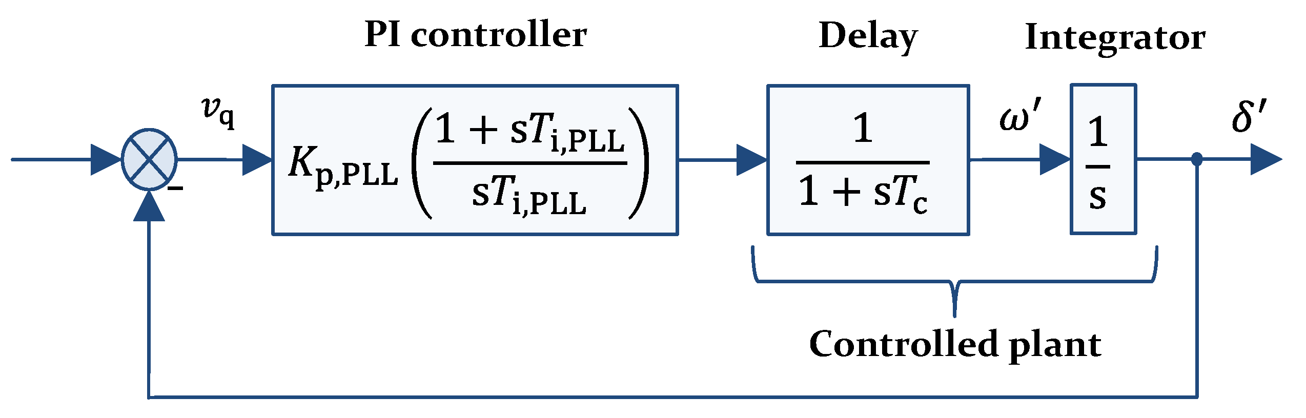
Phase Locked Loop (PLL)
2.3.2. Battery Storage Systems
Current Controller
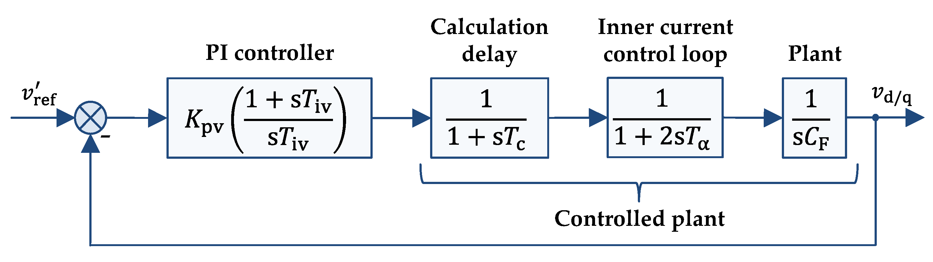
AC Voltage Controller
2.4. Fault Behaviour of Microgrids in the Island Mode
2.5. Effect of Pooling Microgrids on the System Stability
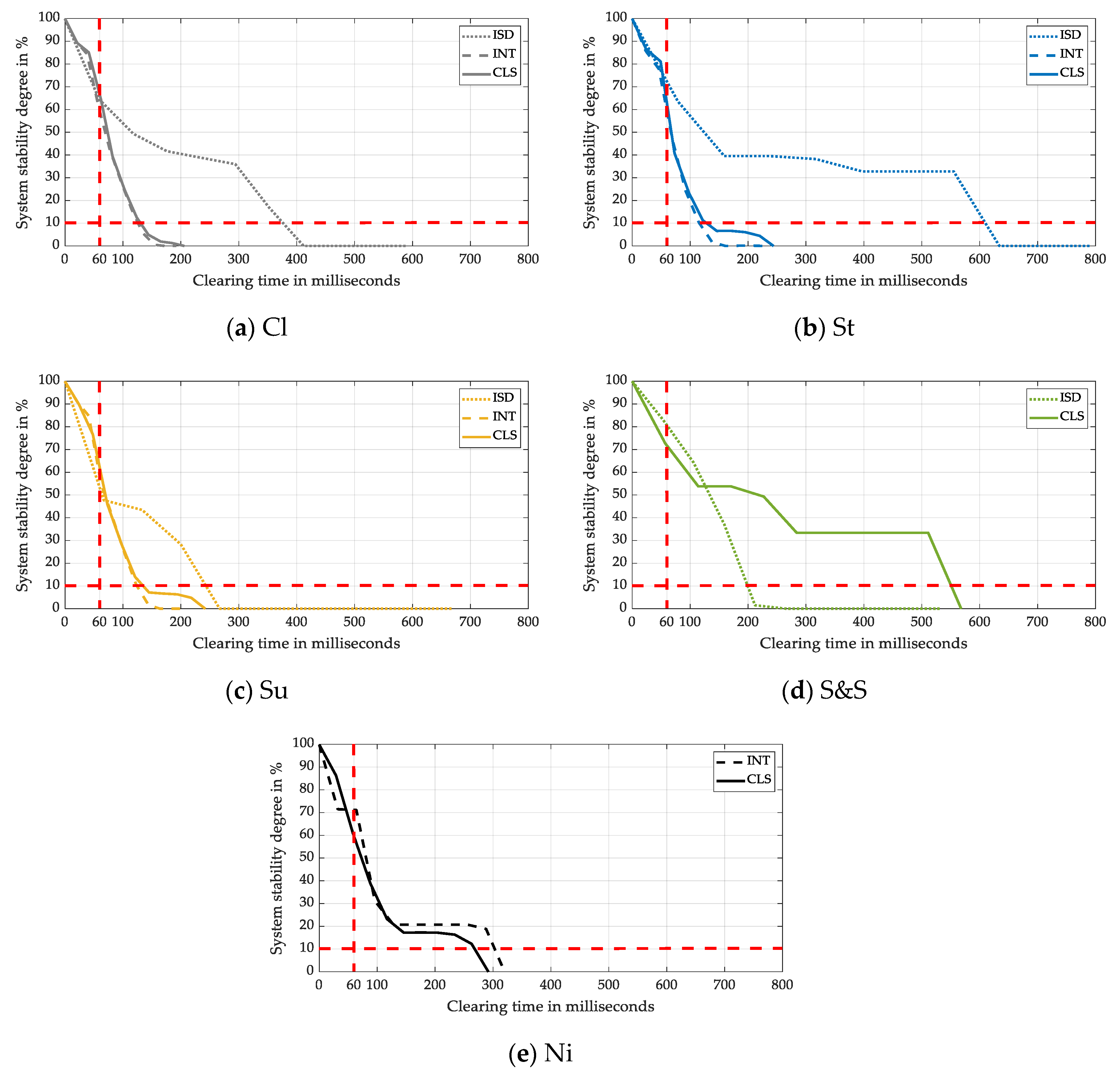
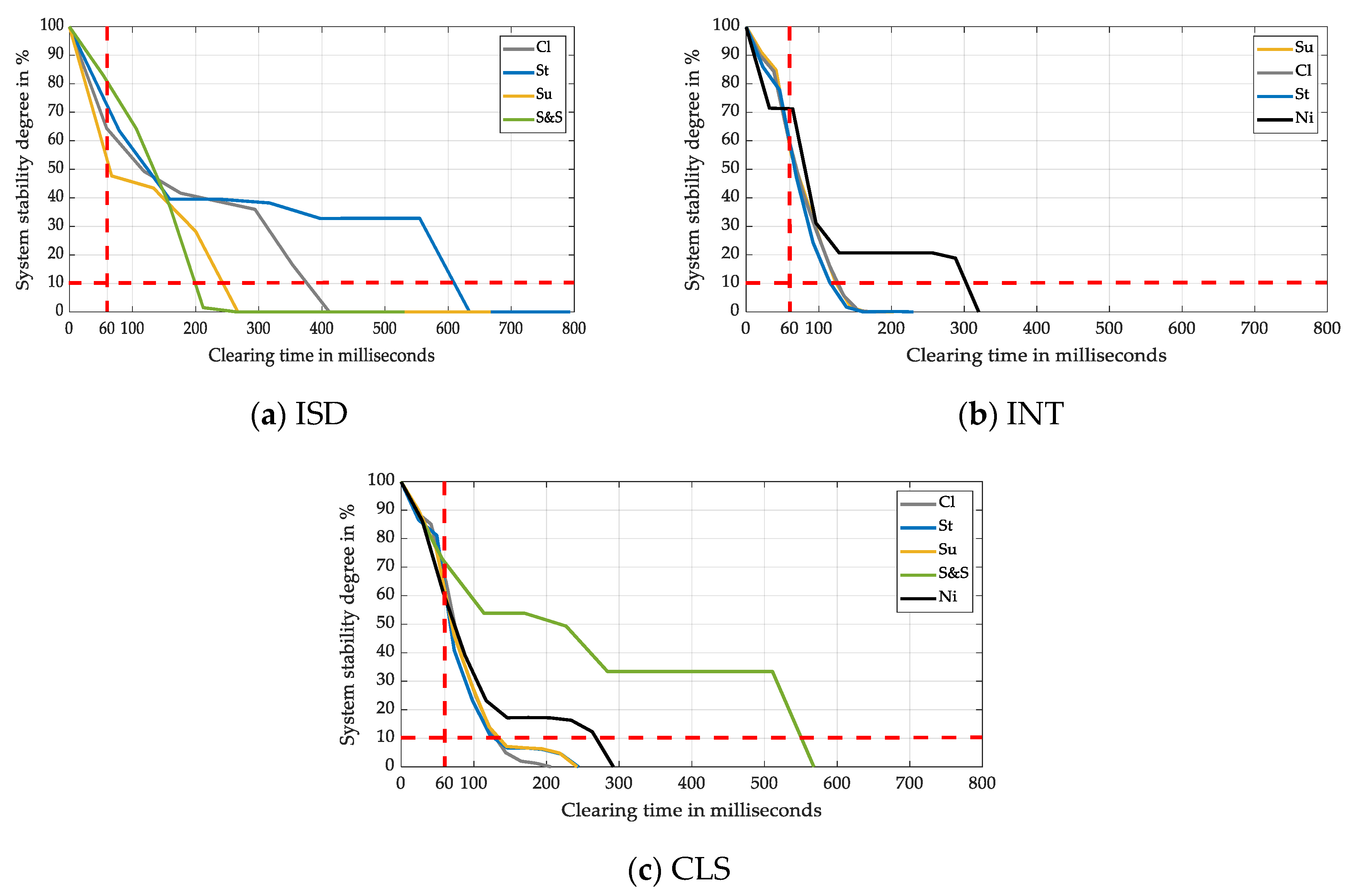
2.6. Quantitative Transient Stability Assessment
3. Results and Discussion
3.1. Critical Clearing Times
3.1.1. Comparison of Scenarios
Island
Interconnection
Cluster
3.1.2. Comparison of Scenarios with Respect to Operating Modes
Interconnection vs. Island
Cluster vs. Island
3.1.3. Comparison of Operating Modes
Classical
Hybrid
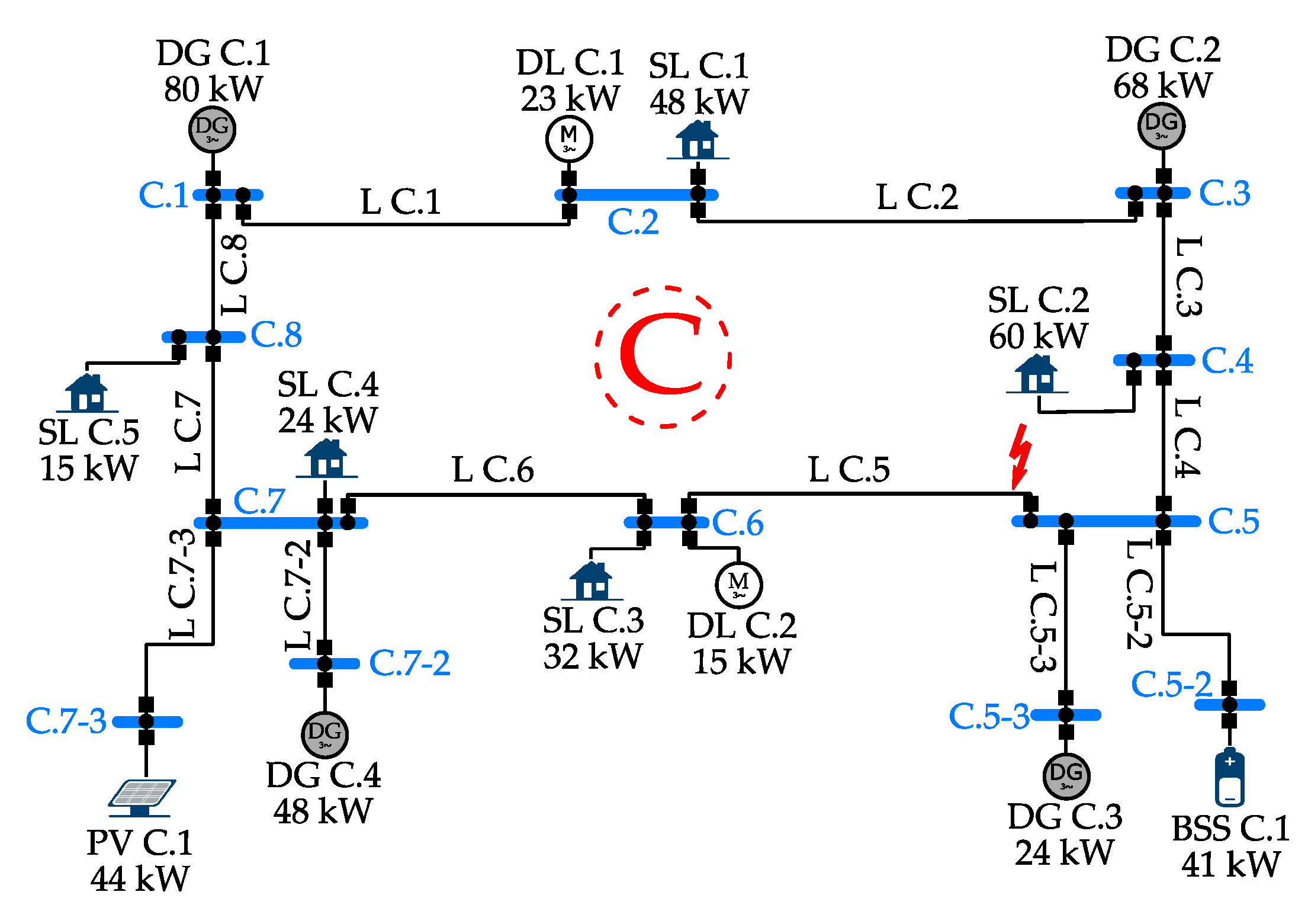
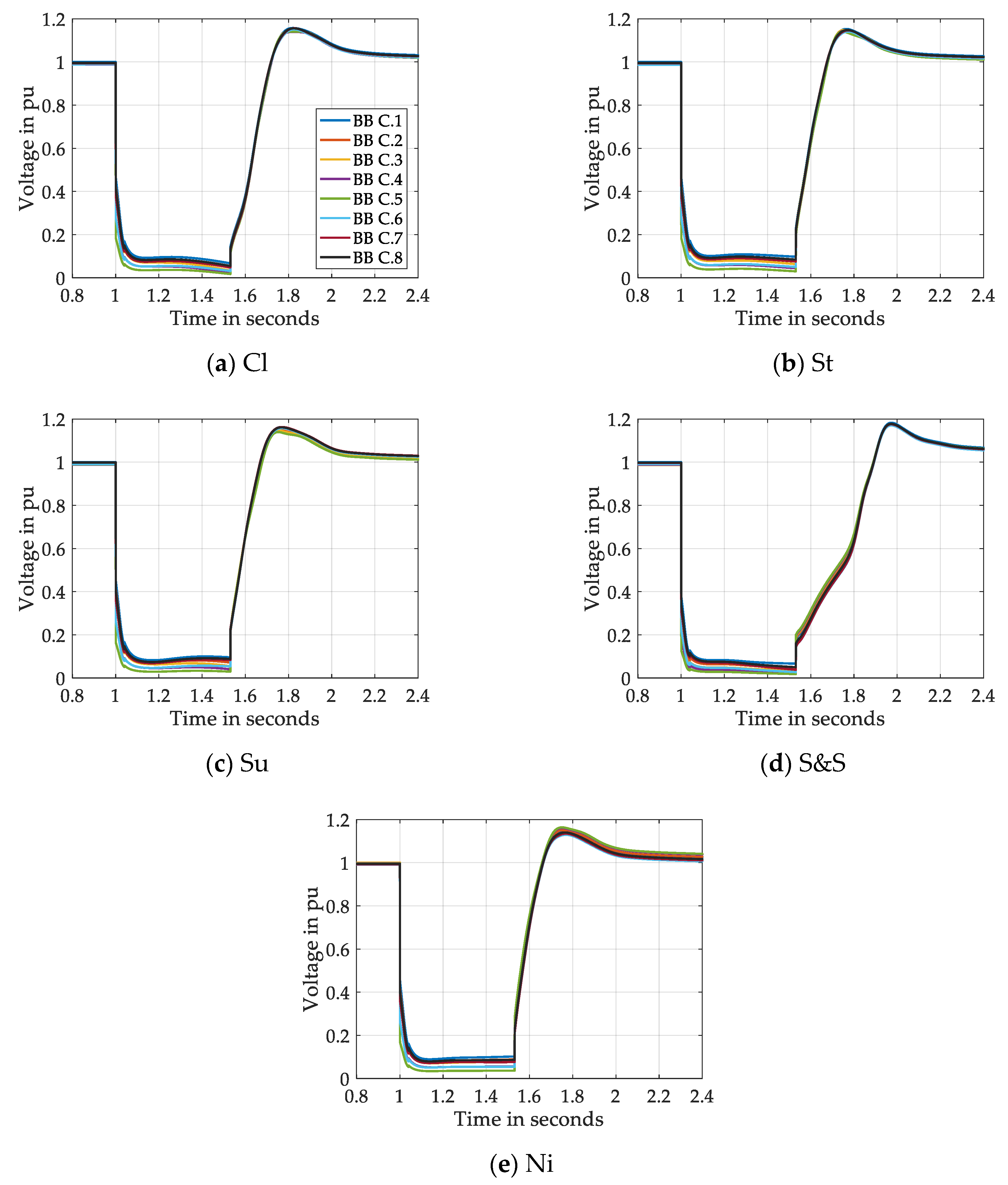
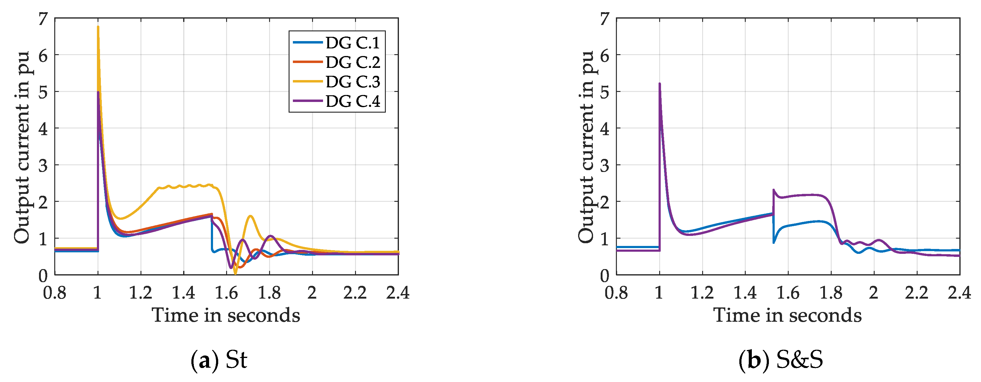
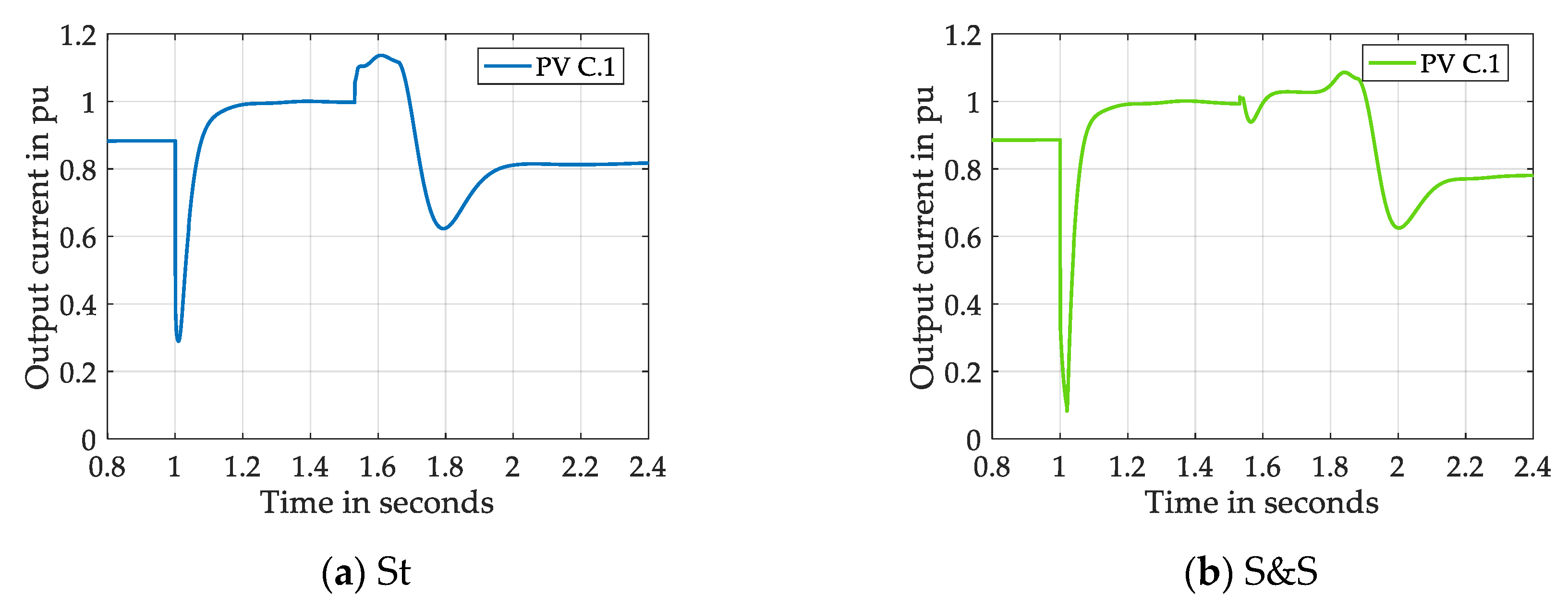
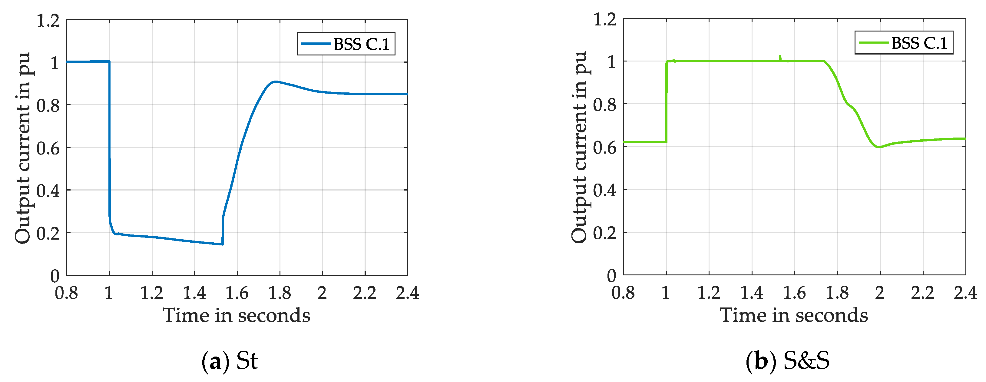
3.2. Fault Behaviour of Microgrid C in Island Mode
3.2.1. Bus Voltage and Frequency
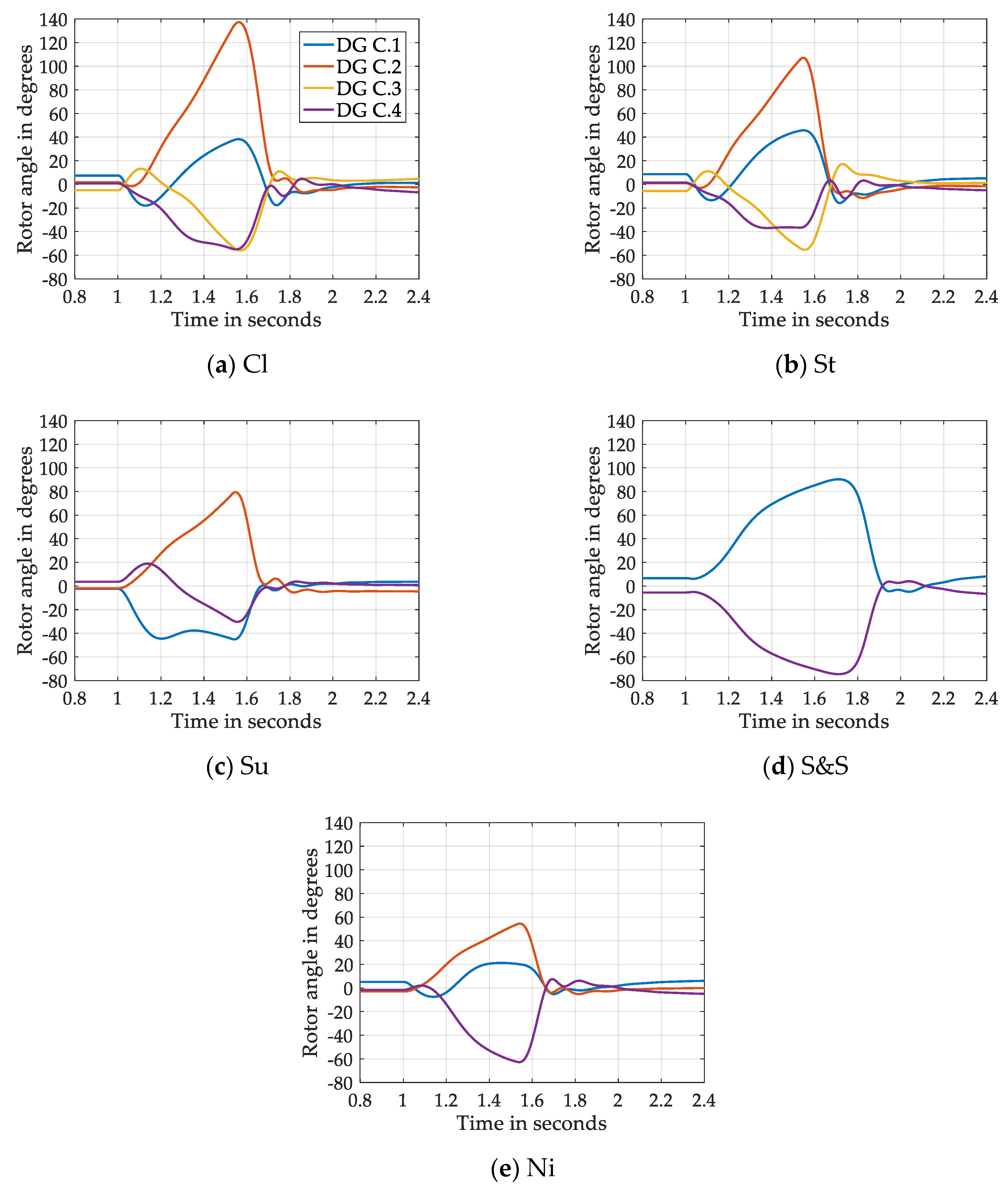
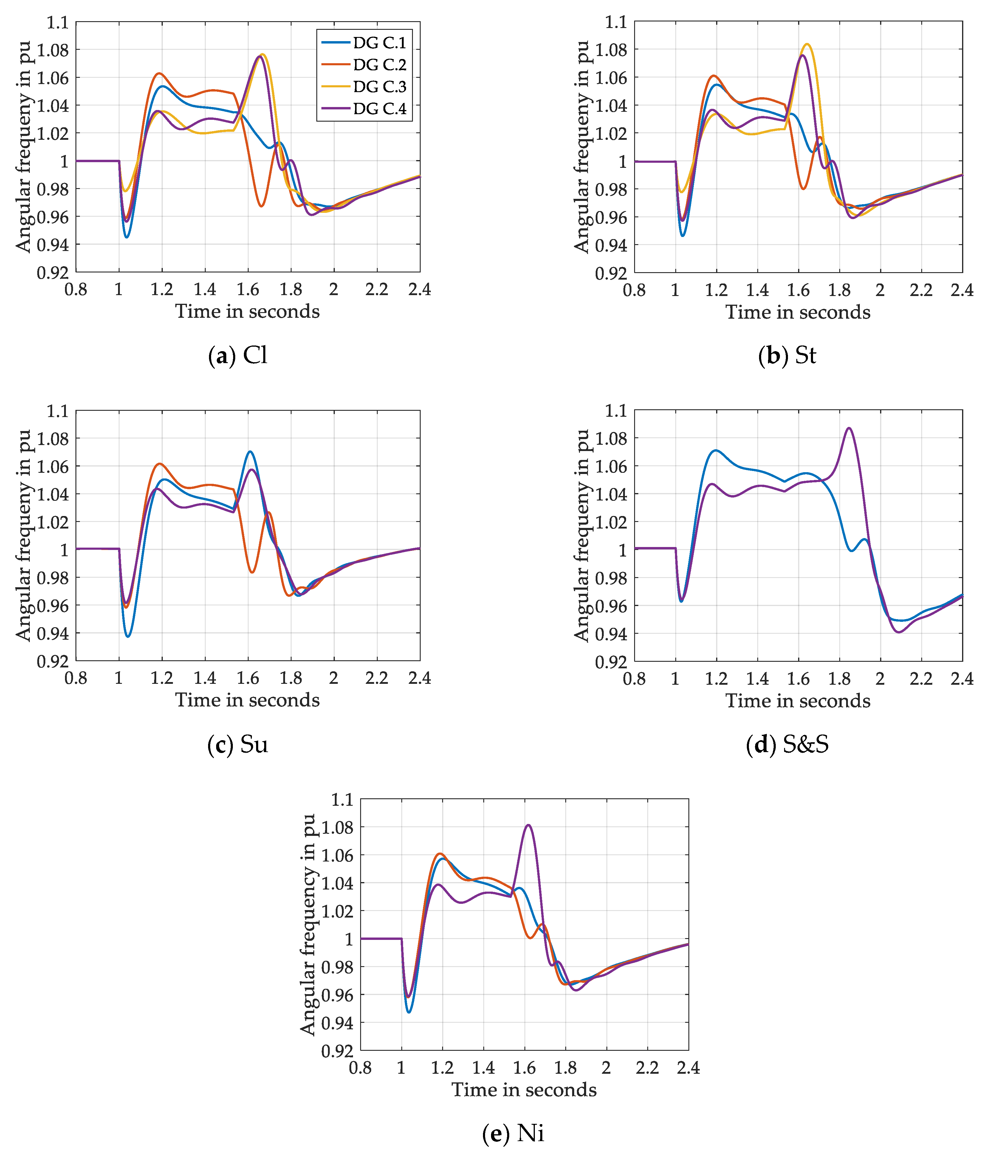
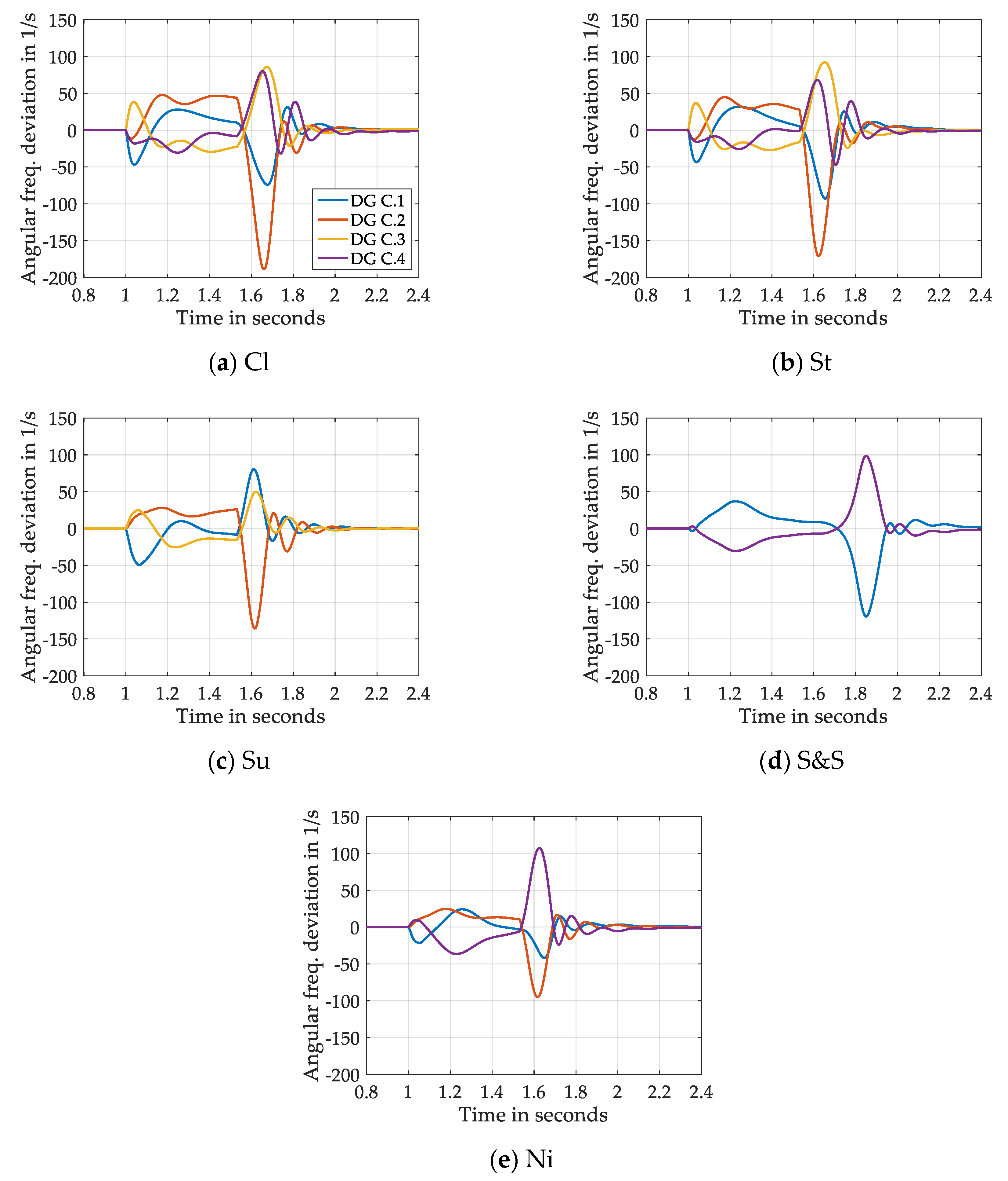
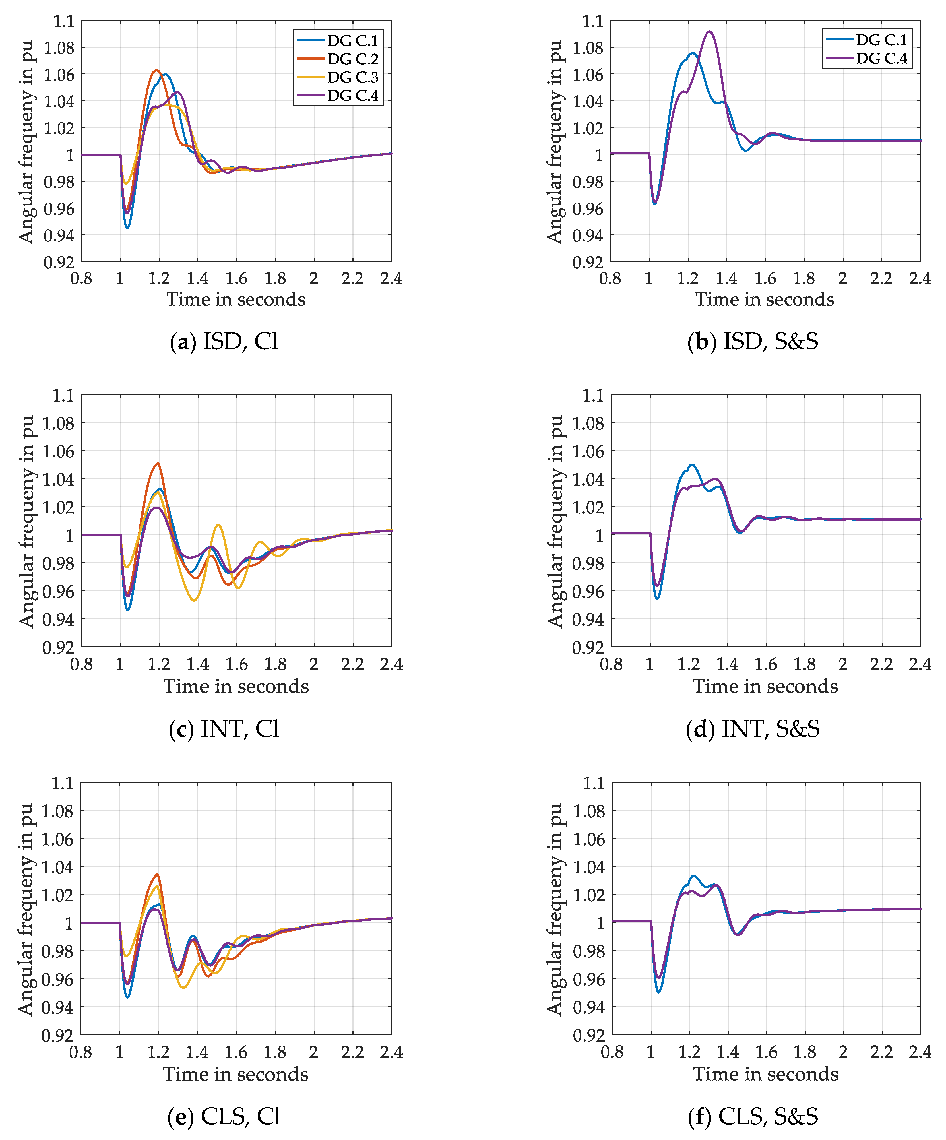
3.2.2. Relative Rotor Angle, Actual Rotor Angular Frequency and Relative Rotor Angular Frequency Deviation of DGs
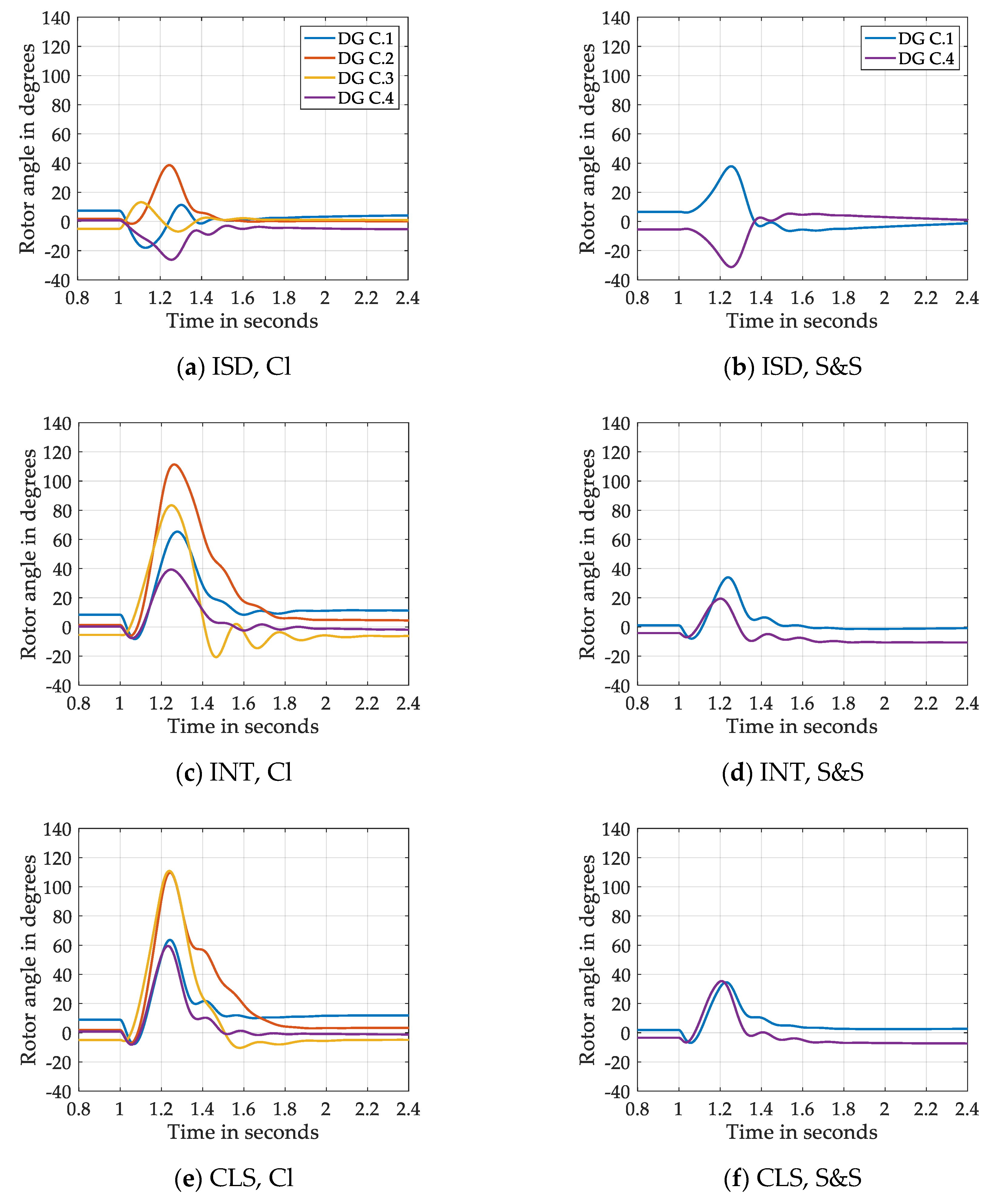
Relative Rotor Angle
Actual Rotor Angular Frequency
Relative Rotor Angular Frequency Deviation
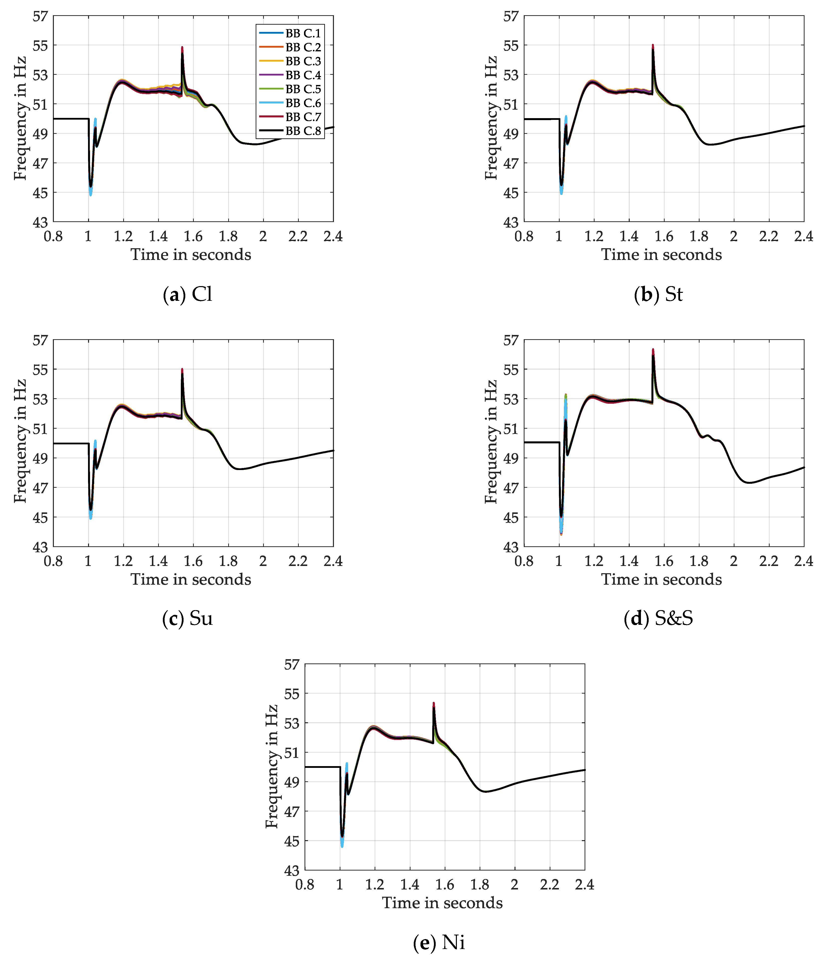
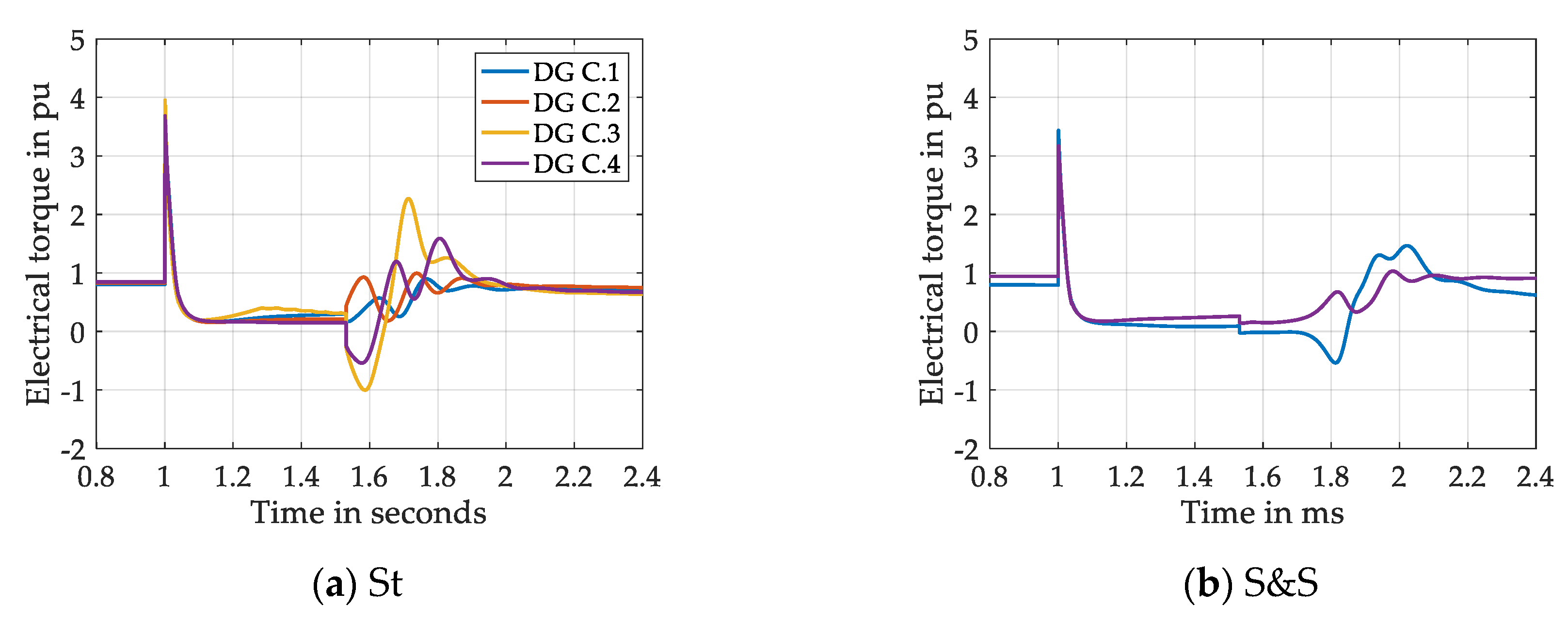
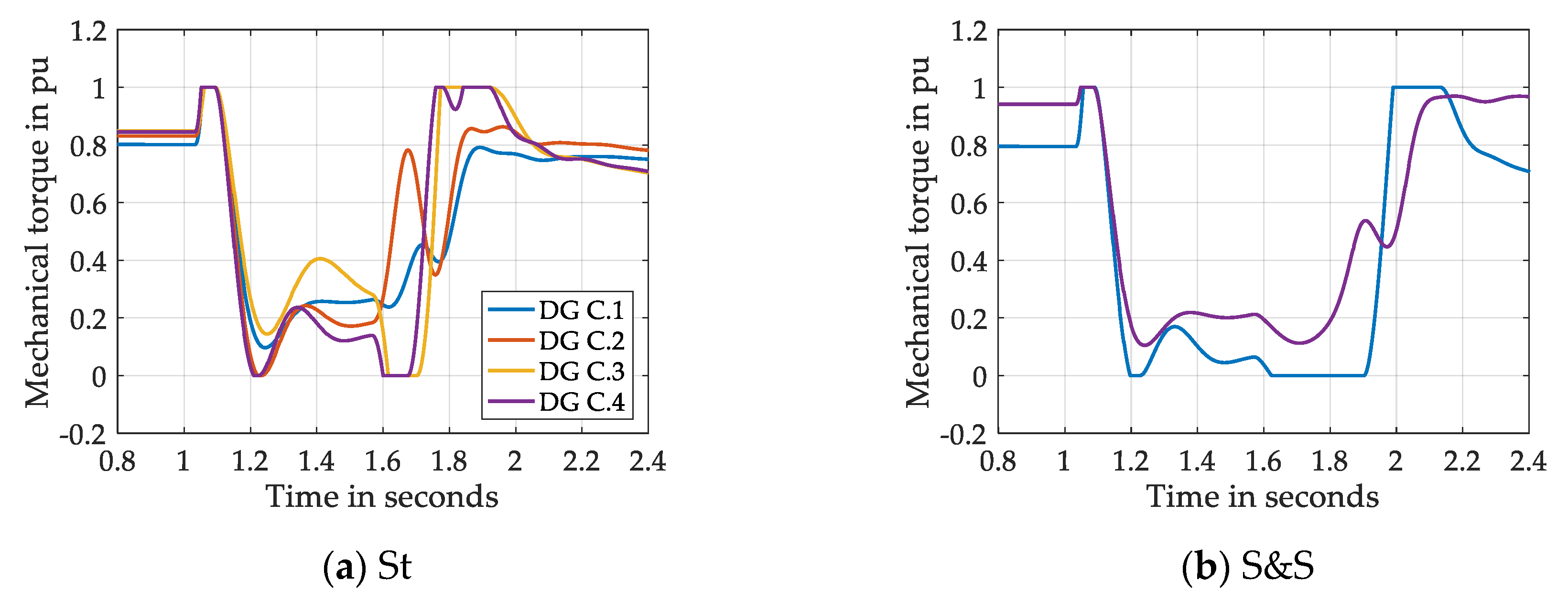
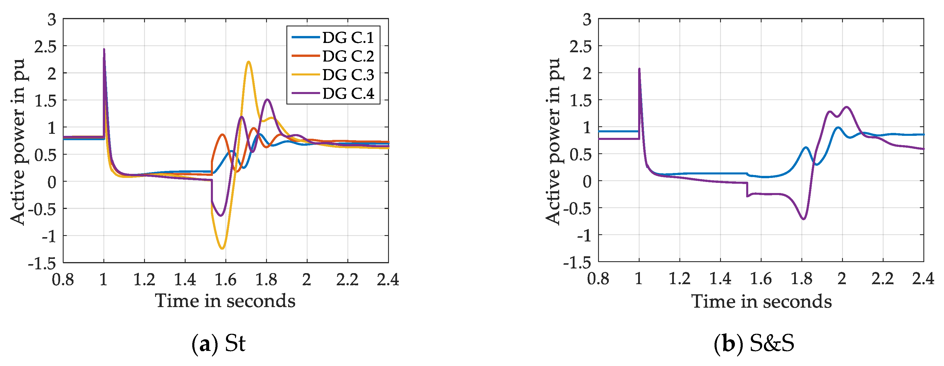
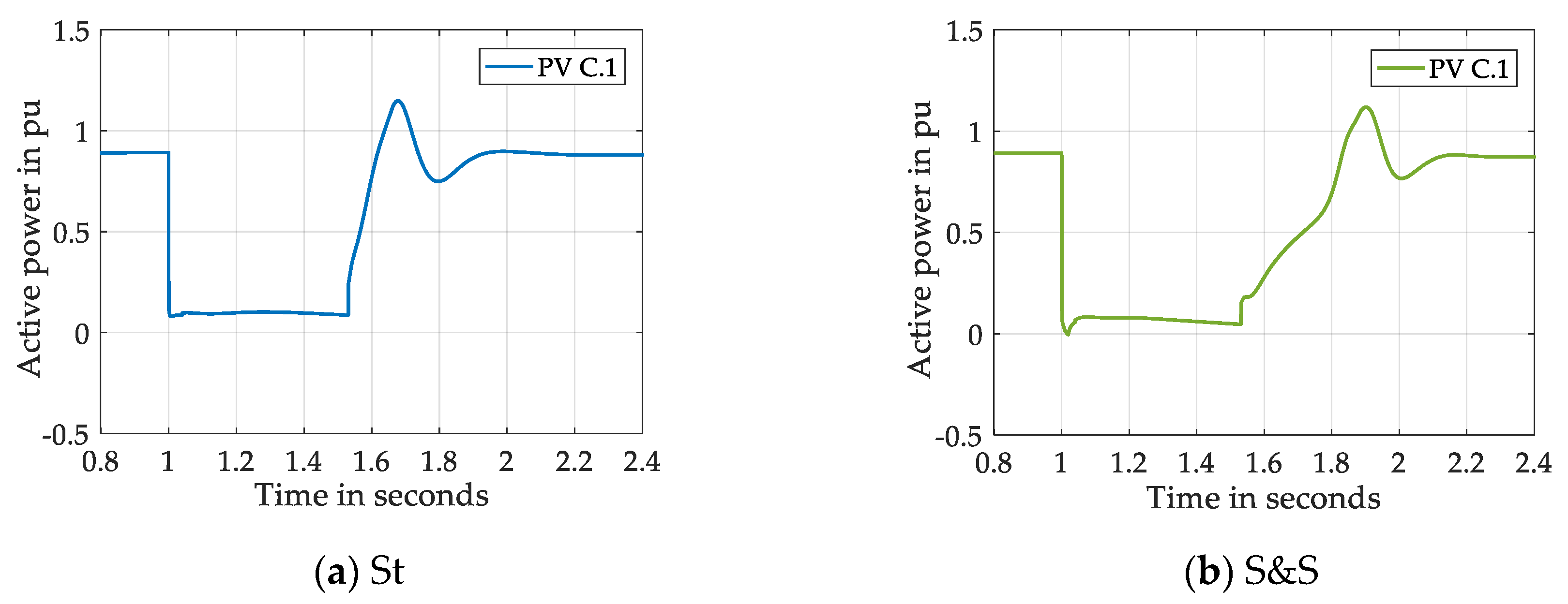
3.3. Effect of Pooling Microgrids on the System Stability
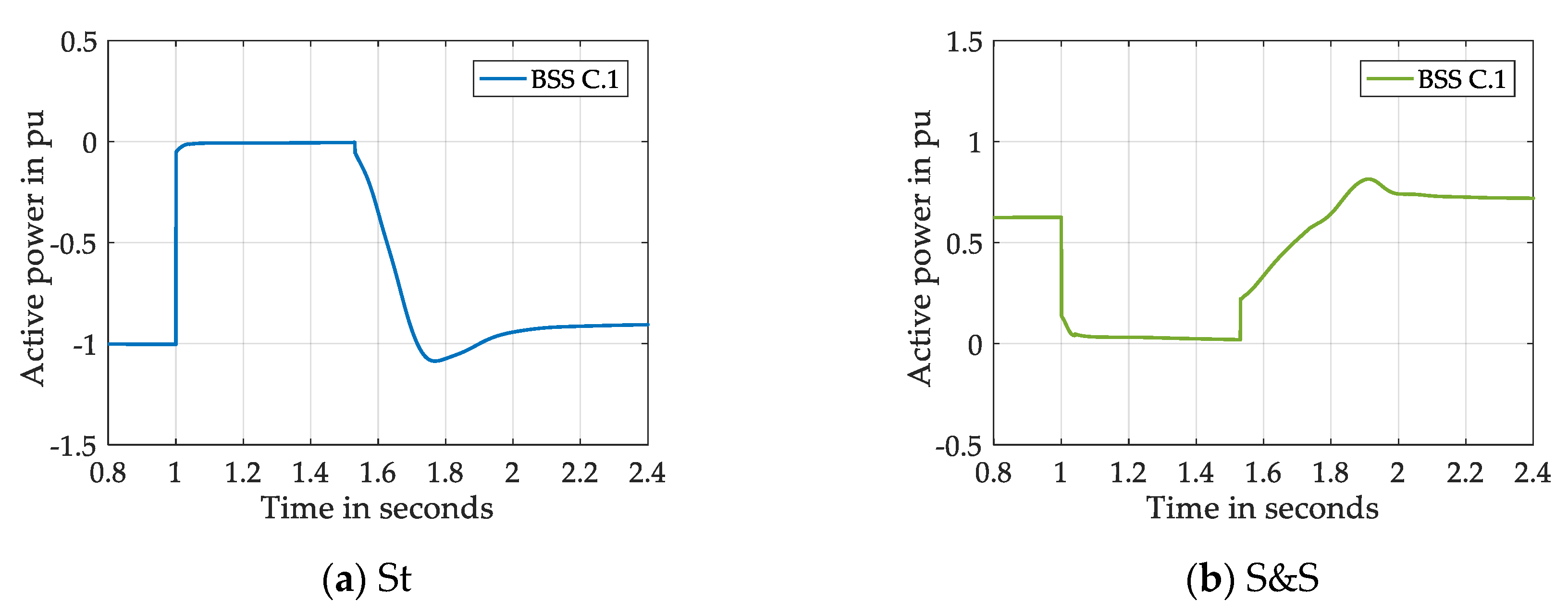
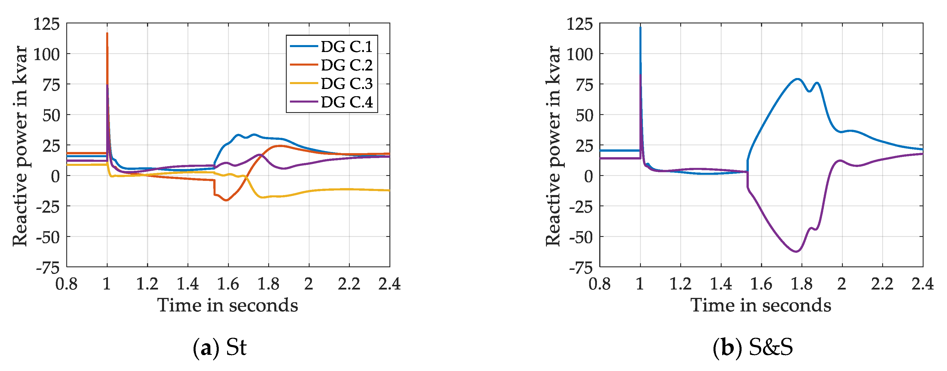
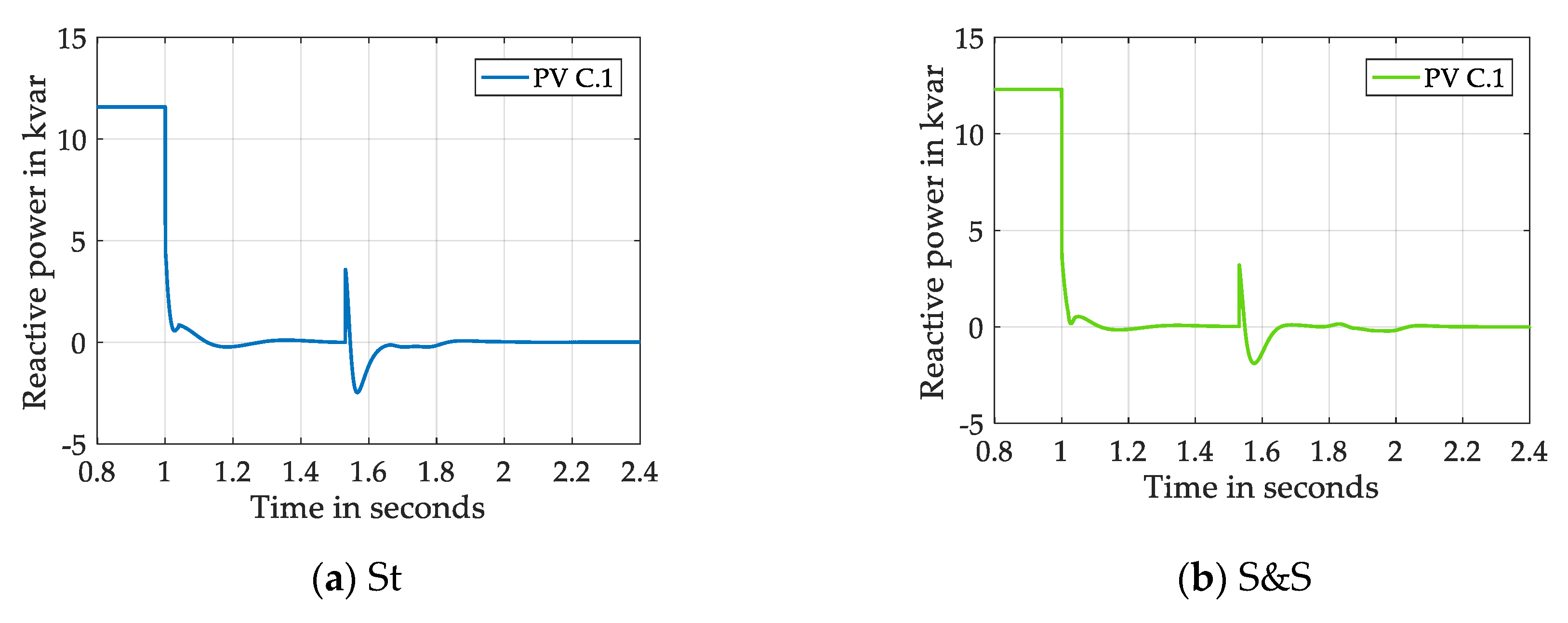
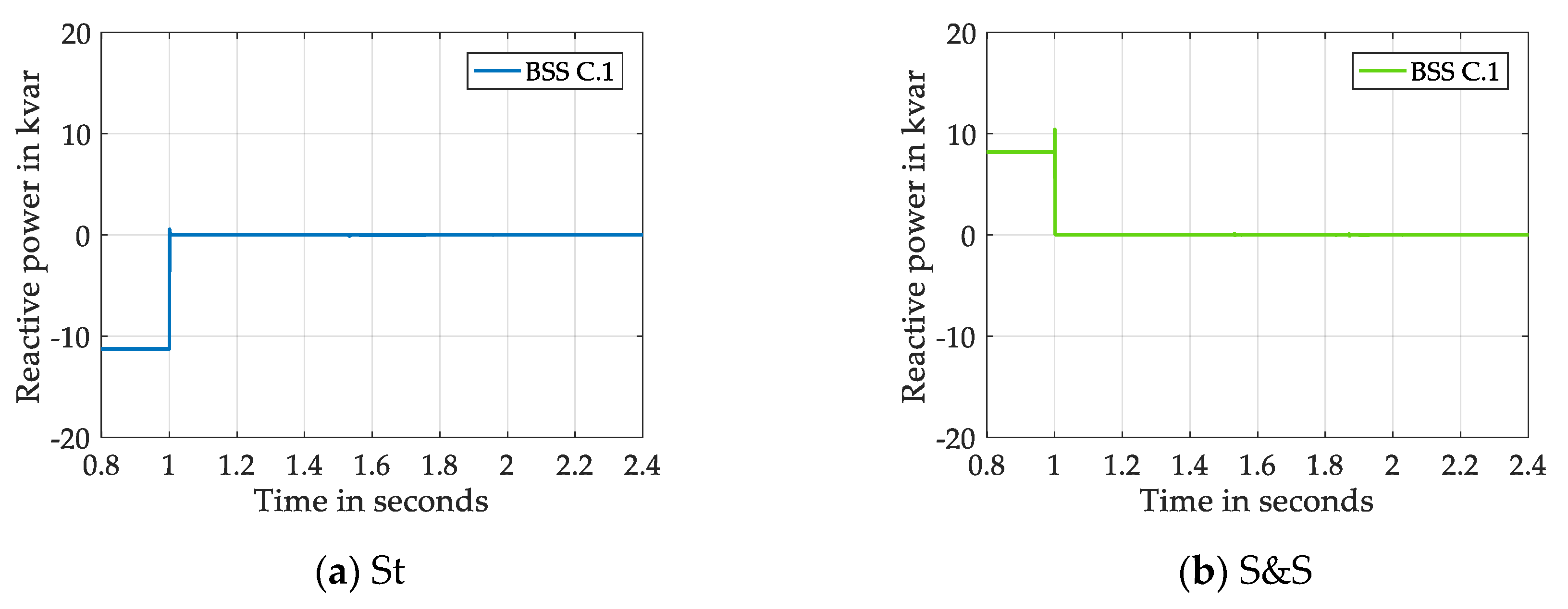
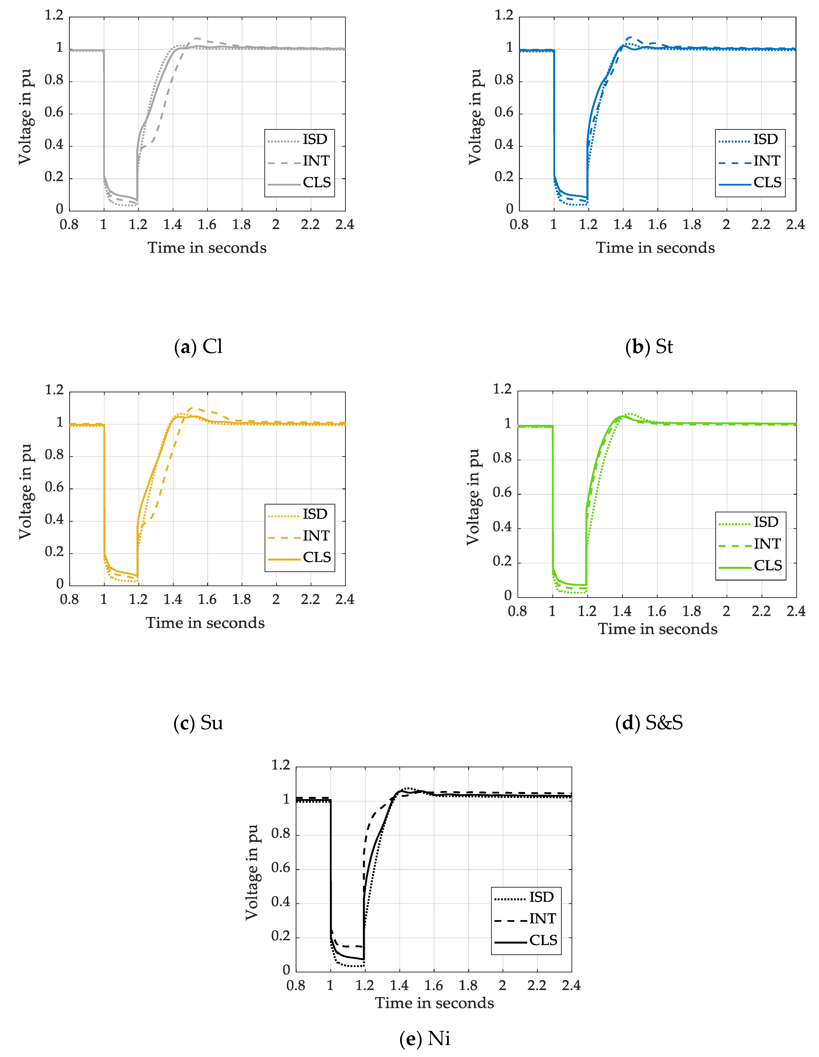
3.3.1. Voltage Stability
3.3.2. Frequency Stability
3.3.3. Rotor Angle Stability
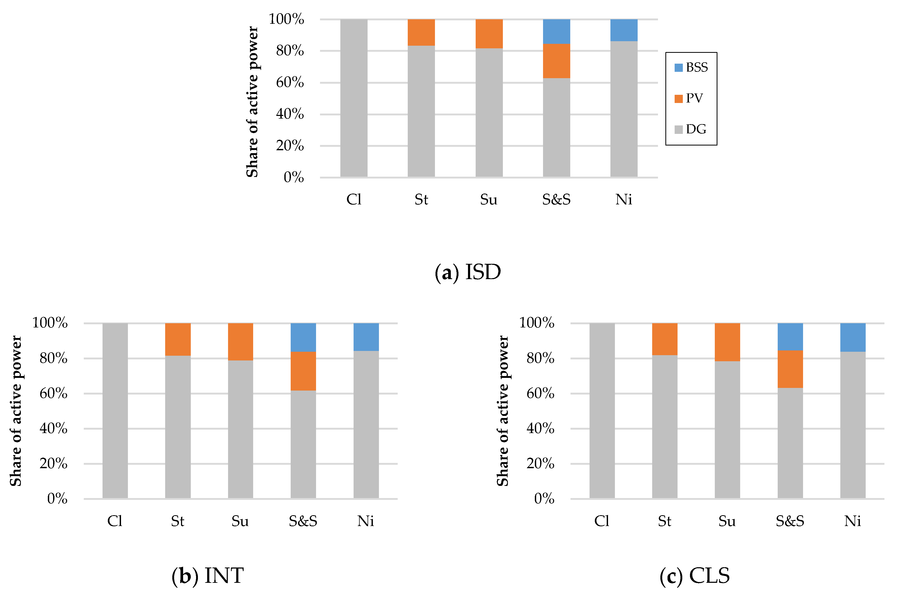
- Storage, sun and night scenario can be chosen in the islanded operation of microgrid C.
- Furthermore, storage, sun and storage, and night scenario outperform the other scenarios in the interconnected operating mode.
- In the clustered operating mode, sun and storage, and night scenario are beneficial.
3.4. System Stability Degree in Operating Modes and Scenarios
3.4.1. Operating Modes
3.4.2. Scenarios
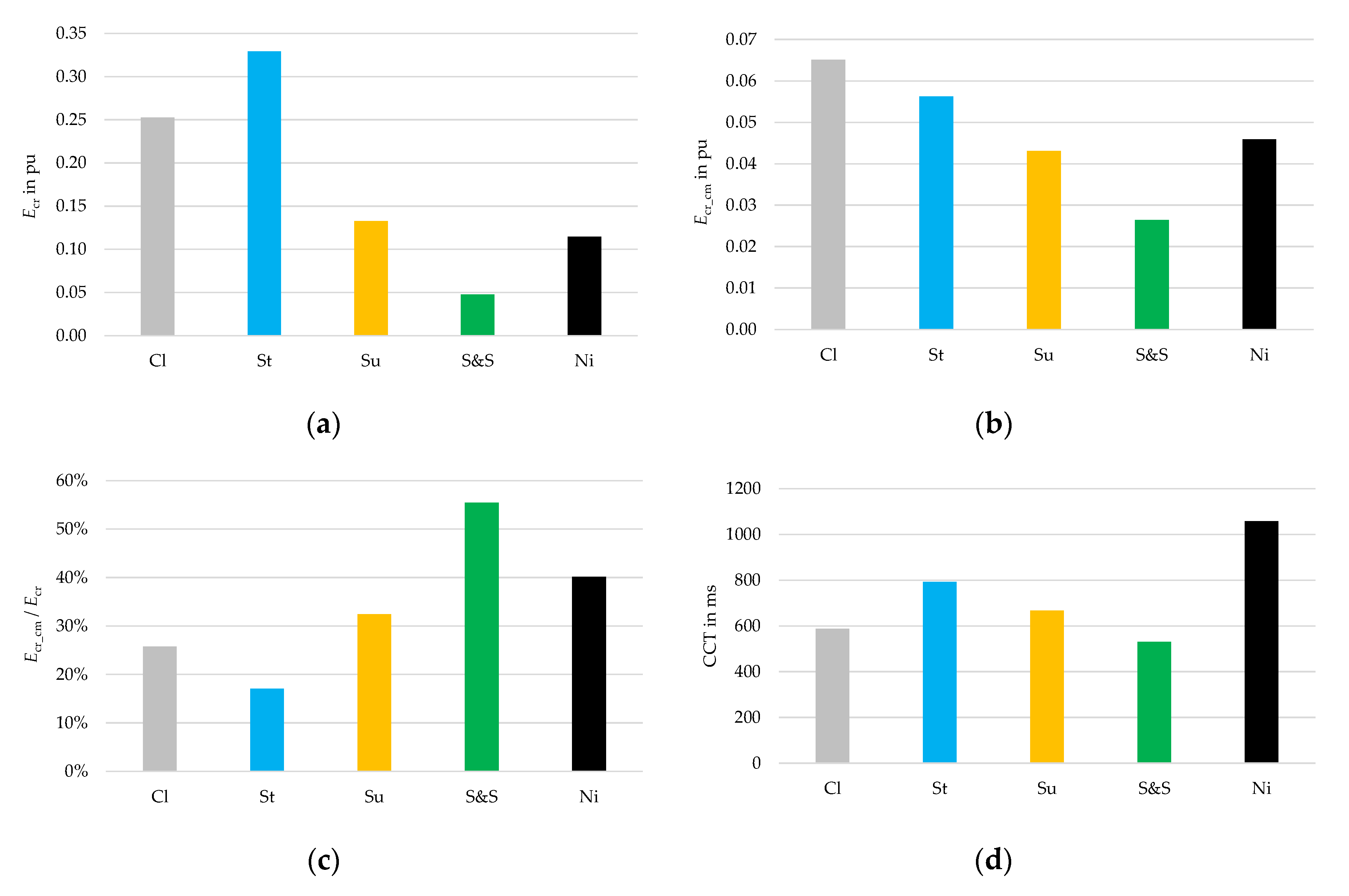
3.5. Comparison of Critical Energy in Scenarios and Operating Modes
3.5.1. Island
3.5.2. Cluster
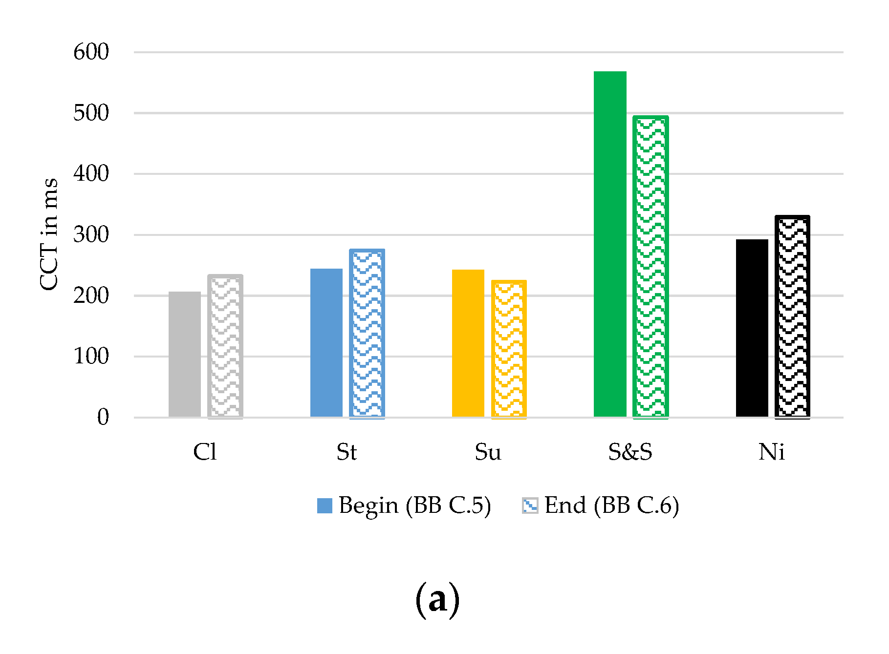
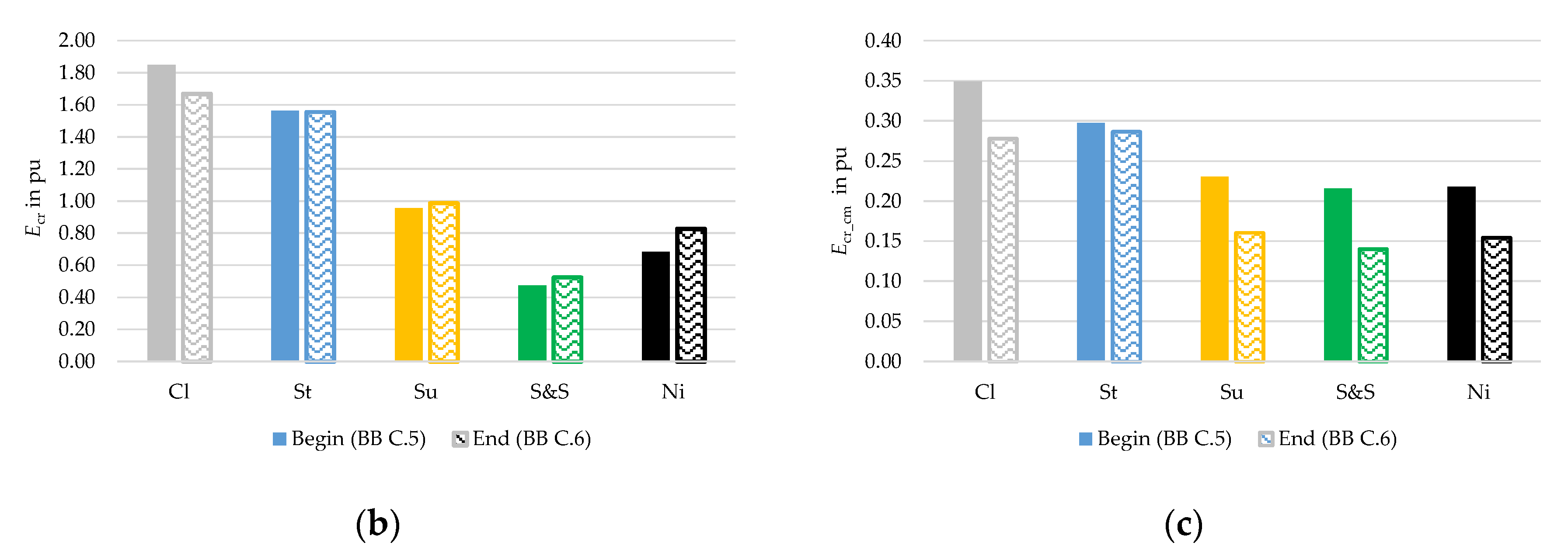
3.6. Influence of Fault Location on Critical Energy in Cluster Mode
4. Summary and Outlook
4.1. Summary
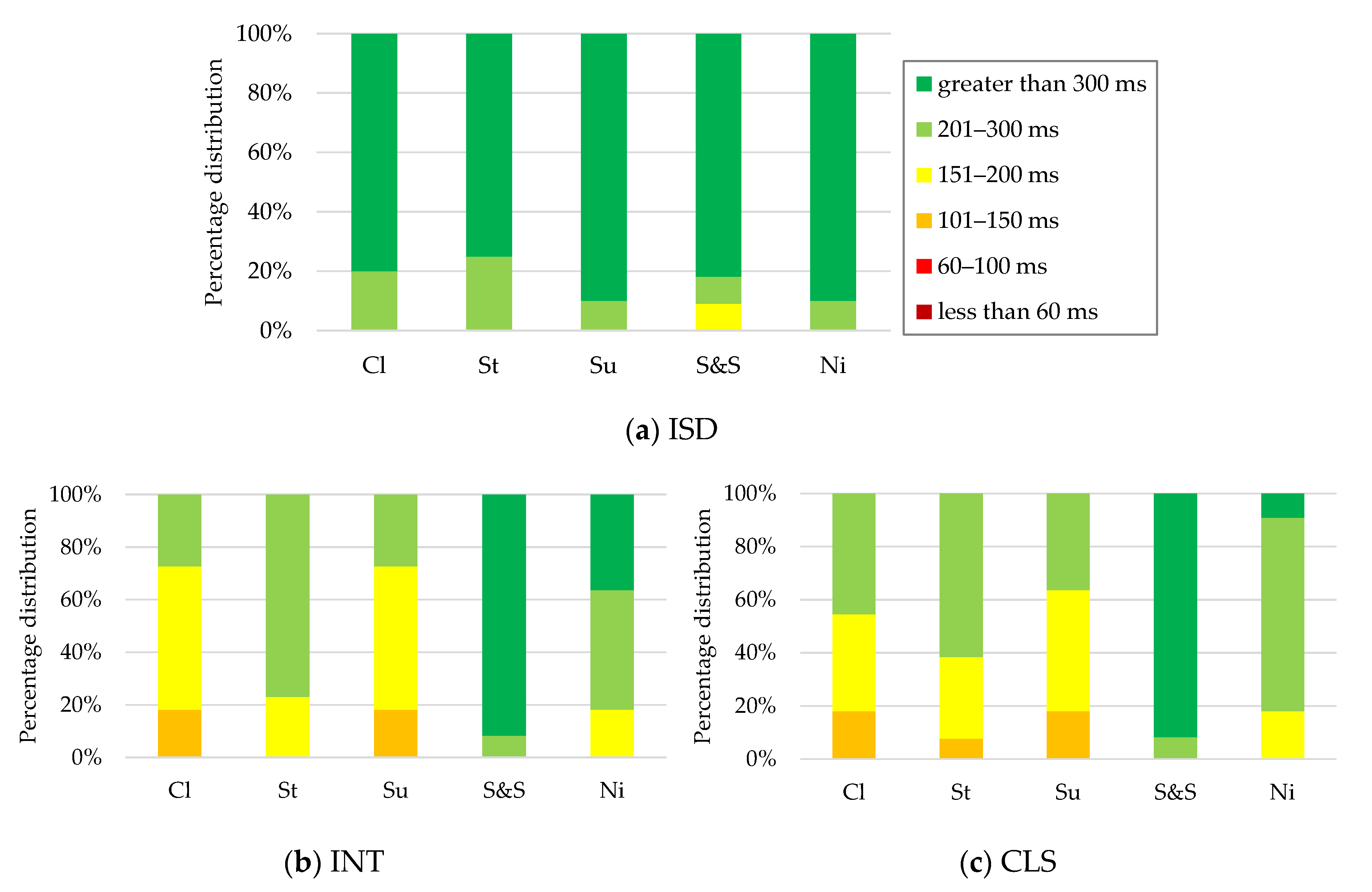
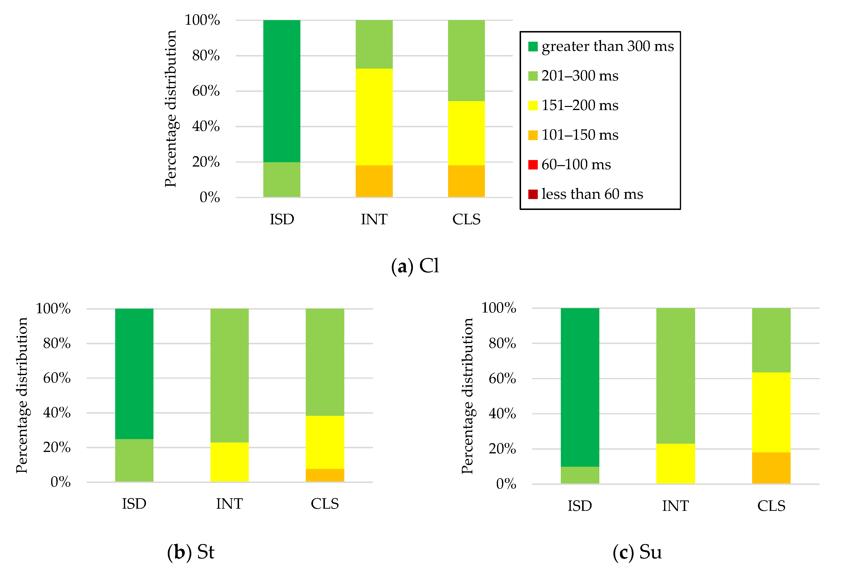
- Critical clearing times: According to the CCT profiles of the microgrids (based on the risk level) with respect to the operating modes and scenarios, it can be concluded that, any scenario can be preferred in the islanded mode. However, scenario “sun & storage” is characterized by better CCT profiles in the interconnected and clustered mode. In general, coupling classical or hybrid microgrids is not critical with respect to the CCT values for the considered high load operating point on a partly sunny day. However, interconnection and cluster mode are characterized by a relatively higher risk of transient stability as against the island mode.
- Fault behavior of microgrid C in island mode: The response of microgrid C—in the pre-fault, fault-on and post-fault period—at both system and equipment level for the simulated short-circuit can be assessed as plausible and thereby the dynamic system modelling can be validated.
- Effect of pooling microgrids on the system stability: Scenarios “storage”, “sun”, and “night” of microgrid C perform better in the islanded operation regarding the critical short-circuit location. On the other hand, scenarios “storage”, “sun & storage”, and “night” outperform in the interconnected mode. Further, scenarios “sun & storage” and “night” have a positive impact on the system stability in the clustered mode. In this studied case, scenario “night” can be categorized to be the most optimal in each operating mode, whereas scenario “classical” does not perform better among the scenarios. Analyses regarding the selection of the optimal operating modes and scenarios should be executed on a regular basis—by considering only the critical fault(s) with respect to either location or CCT values—in the near real-time grid operation.
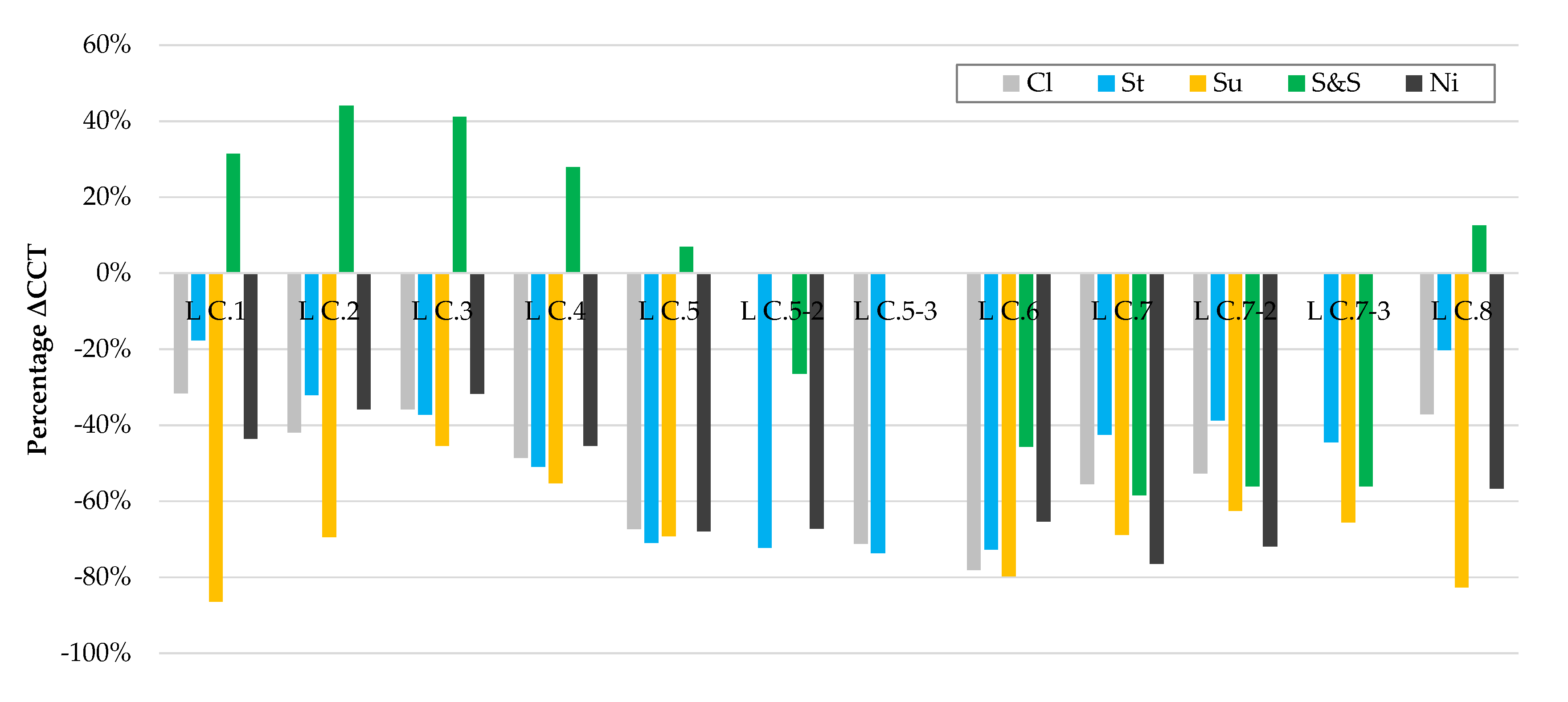
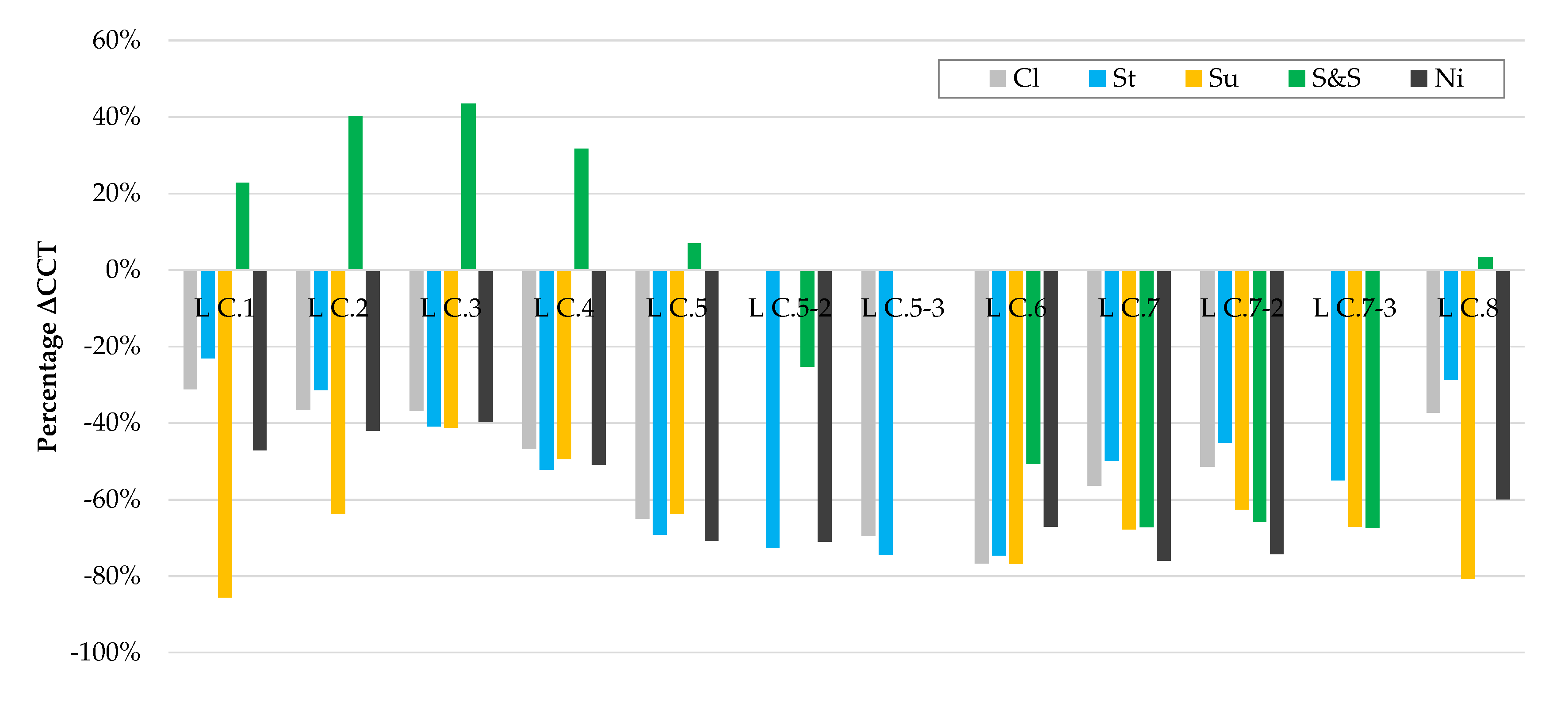
- System stability degree in operating modes and scenarios: The SSD was determined for each corresponding (stable) fault clearing time in various cases with the help of the micro-hybrid method. The SSD profile of the scenarios in interconnection and cluster mode is, in terms of the severity of the fault and sensitivity of the system, more critical than that in island mode, which is characterized by the slope of the profiles. The relative difference between the CCT and the corrected critical clearing time (CCCT) of the cases, calculated based on the threshold value of the SSD, lies between 3% and 64%. It is recommended to take CCCT into account while setting the protection systems in microgrids, so that the risk of system losing stability can be reduced even further. In addition, the gradient of the SSD profiles should be considered while selecting the optimal scenario in the operating modes and scenarios.
- Comparison of critical energy in scenarios and operating modes: According to the analyses of the absolute value of the critical energy of the system and of the critical machine as well as the CCT (of the studied fault in different scenarios and operating modes), it can be inferred that, the ratio of the critical energy of the critical machine to that of the system lies between 20% and 60%. The ratio is relatively higher in the scenarios with a smaller number of active DGs.
- Influence of fault location on critical energy in cluster mode: In case of a one-machine infinite bus system, an inverse proportionality between the CCT and critical energy of the machine (simplified 2nd order model) can be observed. Further, the ratio of the CCT of the critical fault to the CCT of the fault with a residual voltage during fault-on period is relatively high. It can be concluded from the simulation results (of two nearby fault locations) that the CCT and critical energy values of the critical machine are both directly and inversely proportional. Finding a direct correlation between the CCT and the critical energy of the system with respect to different fault locations, especially in cluster mode, can be misleading. However, investigation of the CCT of critical faults as well as the critical energy of every DG or a group of “critical” DGs can help to set optimal steady-state operating points of DGs—in the grid planning phase or in the near real-time operation.
- Coupling classical or hybrid microgrids is, in principle, technically feasible regarding CCT. However, interconnection and cluster mode exhibit a relatively higher risk of transient stability as against the island mode.
- The hybrid scenarios have a more positive effect on the system stability than scenario “classical”. Furthermore, scenario “night” (DGs and BSS) can be ranked as the most optimal in each operating mode, while scenario “classical” (DGs only) has an overall negative effect compared to the other scenarios.
- According to the quantitative TSA, the profiles of SSD versus clearing times of the scenarios in island mode are better than the SSD profiles in interconnection and cluster mode—with respect to the CCT, the CCCT, and the slope of SSD profiles. In spite of the relatively higher gradient, the SSD profiles in the coupled modes are also acceptable.
- Further, according to the results regarding the effect of the fault location on the critical energy, there exists a direct and indirect proportionality between the CCT and critical energy values of the critical machine.
4.2. Outlook
Author Contributions
Funding
Conflicts of Interest
References
- International Renewable Energy Agency (IRENA). Off-Grid Renewable Energy Systems:Status and Methodological Issues. Available online: https://www.irena.org/-/media/Files/IRENA/Agency/Publication/2015/IRENA_Off-grid_Renewable_Systems_WP_2015.pdf (accessed on 13 January 2020).
- Carnegie Mellon University (CMU). Available online: https://www.cmu.edu/ceic/assets/docs/publications/reports/2014/micro-grids-rural-electrification-critical-rev-best-practice.pdf (accessed on 13 January 2020).
- Motoren- und Turbinen-Union (MTU). Available online: https://www.mtu-solutions.com/eu/en/stories/power-generation/gas-generator-sets/microgrid-cooperation-with-qinous.html (accessed on 13 January 2020).
- Caterpillar. Available online: https://www.cat.com/en_US/by-industry/electric-power-generation/Articles/White-papers/white-paper-hybrid-microgrids-the-time-is-now.html (accessed on 13 January 2020).
- United Nations (UN). Available online: https://sustainabledevelopment.un.org/content/documents/interconnections.pdf (accessed on 13 January 2020).
- Microgrid Knowledge. Available online: https://microgridknowledge.com/bronzeville-microgrid-cluster/ (accessed on 13 January 2020).
- Ejal, A.A.; Yazdavar, A.H.; El-Saadany, E.F.; Ponnambalam, K. On the Loadability and Voltage Stability of Islanded AC–DC Hybrid Microgrids During Contingencies. IEEE Syst. J. 2019, 13, 4248–4259. [Google Scholar] [CrossRef]
- Saleh, M.S.; Althaibani, A.; Esa, Y.; Mhandi, Y.; Mohamed, A. Impact of Clustering Microgrids on Their Stability and Resilience during Blackouts. In Proceedings of the International Conference on Smart Grid and Clean Energy Technologies, Offenburg, Germany, 20–23 October 2015; pp. 195–200. [Google Scholar]
- Shafiee, Q.; Dragicevic, T.; Vasquez, J.C.; Guerrero, J.M. Hierarchical Control for Multiple DC-Microgrids Clusters. IEEE Trans. Energy Convers. 2014, 29, 922–933. [Google Scholar] [CrossRef]
- Shafiee, Q.; Dragicevic, T.; Vasquez, J.C.; Guerrero, J.M. Modeling, Stability Analysis and Active Stabilization of Multiple DC-Microgrid Clusters. In Proceedings of the ENERGYCON, Dubrovnik, Croatia, 13–16 May 2014; pp. 1284–1290. [Google Scholar]
- Nikolakakos, I.P.; Zeineldin, H.H.; El-Moursi, M.S.; Hatziargyriou, N.D. Stability Evaluation of Interconnected Multi-Inverter Microgrids through Critical Clusters. IEEE Trans. Power Syst. 2016, 31, 3060–3072. [Google Scholar] [CrossRef]
- Zhao, Z.; Yang, P.; Wang, Y.; Xu, Z.; Guerrero, J.M. Dynamic Characteristics Analysis and Stabilization of PV-Based Multiple Microgrid Clusters. IEEE Trans. Smart Grid 2017, 10, 805–818. [Google Scholar] [CrossRef]
- He, J.; Wu, X.; Wu, X.; Xu, Y.; Guerrero, J.M. Small-Signal Stability Analysis and Optimal Parameters Design of Microgrid Clusters. IEEE Access 2019, 7, 36896–36909. [Google Scholar] [CrossRef]
- Majumder, R. Some aspects of stability in microgrids. IEEE Trans. Power Syst. 2013, 28, 3243–3252. [Google Scholar] [CrossRef]
- Pavella, M.; Ernst, D.; Ruiz-Vega, D. Transient Stability of Power Systems: A Unified Approach to Assessment and Control; Kulwer: Norwell, MA, USA, 2000. [Google Scholar]
- CIGRE. Available online: https://e-cigre.org/publication/325-review-of-on-line-dynamic-security-assessment-tools-and-techniques (accessed on 13 January 2020).
- Veerashekar, K.; Bichlmaier, A.; Luther, M. Transient stability of hybrid stand-alone microgrids considering the DC-side of photovoltaics. In Proceedings of the 4th International Hybrid Power Systems Workshop, Crete, Greece, 22–23 May 2019; pp. 1–10. [Google Scholar]
- Veerashekar, K.; Eichner, S.; Luther, M. Modelling and transient stability analysis of interconnected autonomous hybrid microgrids. In Proceedings of the 13th IEEE PES PowerTech Conference, Milan, Italy, 23–27 June 2019; pp. 1–6. [Google Scholar]
- Veerashekar, K.; Schuehlein, P.; Luther, M. Quantitative transient stability assessment in microgrids combining both time-domain simulations and energy function analysis. Int. J. Electr. Power Energy Syst. 2020, 115, 1–12. [Google Scholar] [CrossRef]
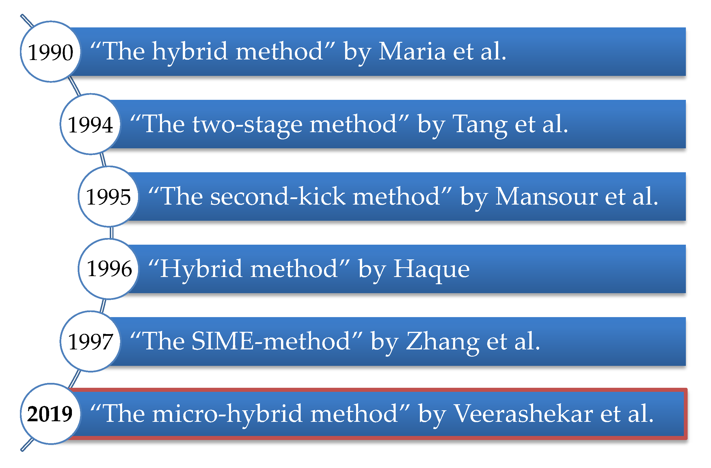
- Veerashekar, K.; Flick, M.; Luther, M. The micro-hybrid method to assess transient stability quantitatively in pooled off-grid microgrids. Int. J. Electr. Power Energy Syst. 2020, 117, 1–12. [Google Scholar] [CrossRef]
- Veerashekar, K.; Flick, M.; Luther, M. Small-signal stability of interconnected autonomous microgrids (German: Kleinsignalstabilität von vernetzten autonomen Mikronetzen). In Proceedings of the International ETG Congress, Esslingen am Neckar, Germany, 8–9 May 2019; pp. 387–392. [Google Scholar]
- Machowski, J.; Bialek, J.W.; Bumby, J.R. Power System Dynamics: Stability and Control, 2nd ed.; Wiley: Chichester, UK, 2012. [Google Scholar]
- German Generator GmbH. Available online: https://germangenerator.com/products/industrial-power-generators/ (accessed on 15 January 2020).
- Sharp. Available online: https://www.sharp.de/cps/rde/xchg/de/hs.xsl/-/html/product-details-solar-modules.htm?product=NQR258H (accessed on 15 January 2020).
- SMA Solar Technology. Available online: https://www.sma.de/en/products/solarinverters/sunny-tripower-60.html (accessed on 16 January 2020).
- SMA Solar Technology. Available online: https://www.sma.de/en/products/solarinverters/sunny-tripower-core1.html (accessed on 16 January 2020).
- IEEE PES. Available online: https://resourcecenter.ieee-pes.org/technical-publications/technical-reports/PES_TR0066_062018.html (accessed on 16 January 2020).
- Stenzel, D.; Hewes, D.; Viernstein, L.; Würl, T.; Witzmann, R. Investigation of demand trends and their impacts on stationary and dynamic aggregated load behaviour. In Proceedings of the International ETG Congress, Esslingen am Neckar, Germany, 8–9 May 2019; pp. 171–176. [Google Scholar]
- DIgSILENT/PowerFactory. Technical Reference Documentation—Asynchronous Machines; DIgSILENT/PowerFactory: Gomaringen, Germany, 2017; pp. 1–36. [Google Scholar]
- Engineers Edge. Available online: https://www.engineersedge.com/motors/classification_electric_motors_13882.htm (accessed on 17 January 2020).
- University of Oviedo. Available online: http://ocw.uniovi.es/pluginfile.php/5424/mod_resource/content/1/Guia%20de%20General%20Electric%20motores%20I.pdf (accessed on 17 January 2020).
- FG Wilson. Available online: http://www.fgwilson.ie/files/generator-set-iso8528-5-2005-operating-limits.pdf (accessed on 17 January 2020).
- International Organization for Standardization (ISO). ISO 8528-5:2013—Reciprocating Internal Combustion Engine Driven Alternating Current Generating Sets—Part 5: Generating Sets; ISO: Geneva, Switzerland, 2013. [Google Scholar]
- Kroutikova, N.; Hernandez-Aramburo, C.A.; Green, T.C. State-space model of grid-connected inverters under current control mode. IET Electr. Power Appl. 2007, 1, 329–338. [Google Scholar] [CrossRef]
- Teodorescu, R.; Liserre, M.; Rodríguez, P. Grid Converters for Photovoltaic and Wind Power Systems; Wiley: Chichester, UK, 2011. [Google Scholar]
- Rocabert, J.; Luna, A.; Blaabjerg, F.; Rodriguez, P. Control of power converters in AC microgrids. IEEE Trans. Power Electron. 2012, 27, 4734–4749. [Google Scholar] [CrossRef]
- Schroeder, D. Electrical Drives—Control of Drive Systems (German: Elektrische Antriebe—Regelung Von Antriebssystemen), 4th ed.; Springer: Berlin, Germany, 2015. [Google Scholar]
- Tripathi, S.M.; Tiwari, A.M.; Singh, D. Optimum design of proportional-integral controllers in grid integrated PMSG-based wind energy conversion system. Int. Trans. Electr. Energy Syst. 2016, 26, 1006–1031. [Google Scholar] [CrossRef]
- Kaura, V.; Blasko, V. Operation of a phase locked loop system under distorted utility conditions. IEEE Trans. Ind. Appl. 1997, 33, 58–63. [Google Scholar] [CrossRef]
- Vinayagam, A.; Swarna, K.S.V.; Khoo, S.Y.; Oo, A.T.; Stojcevski, A. PV based microgrid with grid-support grid-forming inverter control (simulation and analysis). Smart Grid Renew. Energy 2017, 8, 1–30. [Google Scholar] [CrossRef]
- Gkountaras, A. Modeling Techniques and Control Strategies for Inverter Dominated Microgrids. Ph.D. Thesis, Technical University of Berlin, Berlin, Germany, 2017. [Google Scholar]
- De Brabandere, K. Voltage and Frequency Droop Control in Low Voltage Grids by Distributed Generators with Inverter Front-End. Ph.D. Thesis, University of Leuven, Leuven, Belgium, 2006. [Google Scholar]
- SMA Solar Technology. Available online: https://files.sma.de/dl/7418/Iscpv-TI-en-17.pdf (accessed on 18 January 2020).
- Low, H. Control of Grid Connected Active Converter. Master’s Thesis, Norwegian University of Science and Technology, Trondheim, Norway, 2013. [Google Scholar]
- Verband der Elektrotechnik Elektronik Informationstechnik (VDE), VDE-AR-N 4105: Power Generating Plants in the Low Voltage Grid (German: Erzeugungsanlagen am Niederspannungsnetz—Technische Mindestanforderungen für Anschluss und Parallelbetrieb von Erzeugungsanlagen am Niederspannungsnetz); VDE Verlag GmbH: Berlin, Germany, 2018.
- Blaschke, H. Motor Protection (German: Motorschutz); VEB Verlag Technik: Berlin, Germany, 1954. [Google Scholar]
- Ziegler, G. Numerical Differential Protection: Principles and Applications, 2nd ed.; Publicis: Erlangen, Germany, 2011. [Google Scholar]
- Larsen & Turbo. Available online: http://corpwebstorage.blob.core.windows.net/media/37784/omega-acb-catalogue.pdf (accessed on 20 January 2020).
- Eaton. Available online: https://www.eaton.com/ecm/groups/public/@pub/@eaton/@holec/documents/content/ct_255776.pdf (accessed on 20 January 2020).
- Meshcheryakov, V.P.; Sibatov, R.T.; Samoilov, V.V.; Topchii, A.S. Calculation of an interruption arc current and time of arc quenching in low-voltage current breakers. Russ. Electr. Eng. 2008, 79, 92–98. [Google Scholar] [CrossRef]
- Maria, G.A.; Tang, C.; Kim, J. Hybrid transient stability analysis. IEEE Trans. Power Syst. 1990, 9, 384–391. [Google Scholar] [CrossRef]
- Tang, C.K.; Graham, C.E.; El-Kady, M. Transient stability index from conventional time domain simulation. IEEE Trans. Power Syst. 1994, 9, 1524–1530. [Google Scholar] [CrossRef]
- Mansour, Y.; Vaahedi, E.; Chang, A.Y.; Corns, B.R.; Garrett, B.W.; Demaree, K.; Athay, T.; Cheung, K. Hydro’s On-line transient stability assessment (TSA) model development, analysis and post-processing. IEEE Trans. Power Syst. 1995, 10, 241–253. [Google Scholar] [CrossRef]
- Haque, M.H. Hybrid method of determining the transient stability margin of a power system. IEE Proc. Gener. Transm. Distrib. 1996, 143, 27–32. [Google Scholar] [CrossRef]
- Zhang, Y.; Wehenkel, L.; Rousseaux, P.; Pavella, M. SIME: A hybrid approach to fast transient stability assessment and contingency selection. Int. J. Electr. Power Energy Syst. 1997, 19, 195–208. [Google Scholar] [CrossRef]
- Kundur, P. Power System Stability and Control; McGraw-Hill: New York, NY, USA, 1994. [Google Scholar]
- DIgSILENT/PowerFactory. Available online: https://www.digsilent.de/en/stability-analysis.html (accessed on 22 January 2020).


| Scenario | Name (Time of Day) | Short Form | Active Equipment |
|---|---|---|---|
| Classical | Classical (-) | Cl | DGs |
| Hybrid | Storage (12 pm) | St | DGs + PV + BSS (load) |
| Sun (2 pm) | Su | DGs + PV | |
| Sun & Storage (3 pm) | S&S | DGs + PV + BSS (generation) | |
| Night (8 pm) | Ni | DGs + BSS (generation) |
| Generation | Load | DG:PV:BSS | ||||
|---|---|---|---|---|---|---|
| DG | PV | BSS | Total | |||
| Microgrid A | 240 | 60 | 56 | 355 | 239 | 67:17:16 |
| Microgrid B | 204 | 44 | 41 | 289 | 201 | 71:15:14 |
| Microgrid C | 220 | 44 | 41 | 305 | 217 | 72:15:13 |
| Cluster | 664 | 148 | 138 | 949 | 656 | 70:16:14 |
| Classical | Storage | Sun | Sun & Storage | Night | |
|---|---|---|---|---|---|
| Island | 4 | 4 | 3 | 2 | 3 |
| Interconnection | 8 | 8 | 6 | 4 | 6 |
| Cluster | 12 | 12 | 8 | 6 | 8 |
| PV A.1 | PV B.1 | PV C.1 | ||||
|---|---|---|---|---|---|---|
| Island | - | - | - | - | 0.21 | 0.004 |
| Interconnection | 0.14 | 0.004 | - | - | 0.15 | 0.004 |
| Cluster | 0.12 | 0.004 | 0.14 | 0.004 | 0.14 | 0.004 |
| PV A.1 | PV B.1 | PV C.1 | ||||
|---|---|---|---|---|---|---|
| Island | - | - | - | - | 1.14 | 2.0 |
| Interconnection | 1.27 | 2.0 | - | - | 1.14 | 2.0 |
| Cluster | 1.27 | 2.0 | 1.14 | 2.0 | 1.14 | 2.0 |
| PV A.1 | 314 | 0.0101 |
| PV B.1 | ||
| PV C.1 |
| BSS A.1 | BSS B.1 | BSS C.1 | ||||
|---|---|---|---|---|---|---|
| Island | - | - | - | - | 0.60 | 0.0012 |
| Interconnection | 0.76 | 0.0012 | - | - | 0.55 | 0.0012 |
| Cluster | 0.68 | 0.0012 | 0.50 | 0.0012 | 0.50 | 0.0012 |
| BSS A.1 | BSS B.1 | BSS C.1 | ||||
|---|---|---|---|---|---|---|
| Island | - | - | - | - | 0.63 | 8.4 |
| Interconnection | 0.91 | 8.4 | - | - | 0.63 | 8.4 |
| Cluster | 0.91 | 8.4 | 0.63 | 8.4 | 0.63 | 8.4 |
| CCT Range | Risk Level |
|---|---|
| less than 60 ms | extreme |
| 60–100 ms | very high |
| 101–150 ms | high |
| 151–200 ms | medium |
| 201–300 ms | low |
| greater than 300 ms | very low |
| Cl | St (12 pm) | Su (2 pm) | S&S (3 pm) | Ni (8 pm) | ||
| Island | ✓ | ✓ | ✓ | |||
| ✓ | ✓ | |||||
| ✓ | ✓ | ✓ | ||||
| Interconnection | ✓ | ✓ | ✓ | |||
| ✓ | ✓ | ✓ | ||||
| ✓ | ✓ | ✓ | ||||
| Cluster | ✓ | ✓ | ✓ | |||
| ✓ | ✓ | ✓ | ||||
| ✓ | ✓ |
| CCT in ms | CCCT in ms | ΔCCT | ||
|---|---|---|---|---|
| Classical | ISD | 588 | 377 | 36% |
| INT | 192 | 126 | 34% | |
| CLS | 206 | 131 | 36% | |
| Storage | ISD | 793 | 610 | 23% |
| INT | 230 | 116 | 50% | |
| CLS | 244 | 129 | 47% | |
| Sun | ISD | 667 | 243 | 64% |
| INT | 205 | 124 | 40% | |
| CLS | 242 | 135 | 44% | |
| Sun & Storage | ISD | 531 | 200 | 62% |
| INT | 568 | - | - | |
| CLS | 571 | 552 | 3% | |
| Night | ISD | 1058 | - | - |
| INT | 321 | 303 | 6% | |
| CLS | 292 | 269 | 8% |
| CCT in ms | CCCT in ms | ΔCCT | ||
|---|---|---|---|---|
| Island | Cl | 588 | 377 | 36% |
| St | 793 | 610 | 23% | |
| Su | 667 | 243 | 64% | |
| S&S | 531 | 200 | 62% | |
| Ni | 1058 | - | - | |
| Interconnection | Cl | 192 | 126 | 34% |
| St | 230 | 116 | 50% | |
| Su | 205 | 124 | 40% | |
| S&S | 568 | - | - | |
| Ni | 321 | 303 | 6% | |
| Cluster | Cl | 206 | 131 | 36% |
| St | 244 | 129 | 47% | |
| Su | 242 | 135 | 44% | |
| S&S | 571 | 552 | 3% | |
| Ni | 292 | 269 | 8% |
© 2020 by the authors. Licensee MDPI, Basel, Switzerland. This article is an open access article distributed under the terms and conditions of the Creative Commons Attribution (CC BY) license (http://creativecommons.org/licenses/by/4.0/).
Share and Cite
Veerashekar, K.; Askan, H.; Luther, M. Qualitative and Quantitative Transient Stability Assessment of Stand-Alone Hybrid Microgrids in a Cluster Environment. Energies 2020, 13, 1286. https://doi.org/10.3390/en13051286
Veerashekar K, Askan H, Luther M. Qualitative and Quantitative Transient Stability Assessment of Stand-Alone Hybrid Microgrids in a Cluster Environment. Energies. 2020; 13(5):1286. https://doi.org/10.3390/en13051286
Chicago/Turabian StyleVeerashekar, Kishan, Halil Askan, and Matthias Luther. 2020. "Qualitative and Quantitative Transient Stability Assessment of Stand-Alone Hybrid Microgrids in a Cluster Environment" Energies 13, no. 5: 1286. https://doi.org/10.3390/en13051286
APA StyleVeerashekar, K., Askan, H., & Luther, M. (2020). Qualitative and Quantitative Transient Stability Assessment of Stand-Alone Hybrid Microgrids in a Cluster Environment. Energies, 13(5), 1286. https://doi.org/10.3390/en13051286