Bi-Level Planning of Multi-Functional Vehicle Charging Stations Considering Land Use Types

Abstract

Locating and planning charging stations for Low-Emission Vehicles (LEVs) such as Battery Electric Vehicle (BEV), Hydrogen Fuel-Cell Vehicle (HFCV), and Natural Gas Vehicle (NGV) are becoming increasingly important for LEV users, government, and the automobile industry. Conventional planning approach of charging station usually plans single functional charging station that can only serve one kind of LEVs, and other factors such as fuel type, driving range, initial fuel tank level, and refueling time of the LEV are less considered in the planning stage. In this article, we propose a bi-level planning model to locate and size Multi-Functional Charging Station (MFCS) which can recharge BEV, HFCV, and NGV at the same time in a medium-sized city with different functional areas (e.g., residential area, industrial area, CBD area). We also established a method for generating a daily route considering vehicle attributes and user habits, and we loaded these traveling data into the upper model to select a set of optimal combinations of refueling station locations with a relatively high success ratio. In the lower model, we introduced the mathematical relationship between number of chargers and average user waiting time, and set the total social cost factor, including investment cost and waiting time cost, to evaluate each optimal combination, and then identified the optimum locational result and defined the size of each station. In the case study, we verify the proposed model in several scenarios and conclude that multifunctional refueling station performs better in terms of investment cost and users’ satisfaction level.

1. Introduction

1.1. Background

In recent years, the phenomenon of climate change and energy shortage has brought tremendous worldwide attention to Low-Emission Vehicles (LEVs) which could bring great environmental and social benefits. The penetration of Battery Electric Vehicle (BEVs) and Natural Gas Vehicle (NGVs) has been growing rapidly [1], and a great number of buses and taxis have been converted to BEVs and NGVs [2]. For LEVs, there are currently more than ten types of alternative fuels in production or under development. It is anticipated that LEVs will take the major automobile market share in the near future [3]. However, the lack of charging station infrastructure is one of the most serious obstacles to the promotion of LEVs [4]. Due to the limited fuel tank and battery range, most of the LEVs technically have a shorter driving range than traditional fossil fuel vehicles. Therefore, effective plans for LEV charging stations are in necessary to support the LEVs promotion.

The analysis of charging demand is the basis of the planning problem. In the classic studies, the charging demand is usually assumed to be a fixed value in order to simplify the problem [5,6]. In [5], the charging demand is associatied with destination, ref. [6] assumed centroids of census blocks as charging stations, ref. [7] assumes that the charging demand appears at the destination. However, some literatures suggest that charging demand should reflect the mobility of alternative vehicles [8,9]. Then, ref. [8] proposed a battery capacity-constrained EV flow capturing location model which is highly related with the charging demand, ref. [9] put emphasis on the relationship between charging demand and trave route. Various of approaches are available to solve the locating problem of charging stations from transportation network point of view, among which the flow refueling location model (FRLM) is one of the mainstream methodologies to solve such problem [10,11]. Then [10] used the FRLM methond, considering multiple deviation paths between each of the origin-destination (O-D) pairs. Then [11] used the FRLM method to get the optimal charging station construction strategy. FRLM method relaxes the commonly adopted assumption that travelers only take the shortest path between any O-D pairs.. The main purpose of FRLM is to find the optimum location of refueling stations that can maximize the successful refueling origin–destinations pairs [12]. However, the evaluation stage for the feasibility of all possible combinations of refueling station location requires a large computational effort. Researchers then proposed an improved FRLM method based on heuristic algorithms to solve this problem [13]. Another mainstream solution method for charging station location problem is set-covering approach. Unlike FRLM, the object of set-covering approach is to minimize the total investment cost of charging stations under the premise that all of the traffic flow is covered. It also leads to heavy computational burden, and to release the burden, authors in paper [14] proposed a feasible method to solve the set-covering problem in a much faster way. While FRLM and set-covering approach mainly focus on the road covering problem, many literatures have introduced total social cost index infrastructures when determining the size and location of refueling stations [15,16,17,18]. Normally, the total social cost consists of investment cost (including fixed investment cost, land rental cost, and chargers purchase cost) and waiting time cost [15]. The planning objective of [16] is to minimize the social costs of the whole PEV charging system. Compared with only construction cost, totoal social cost reflects more information when selecting the optimum plan [17]. Then [18] proposed a cost–benefit analysis method to evluate the installation of additional quick-charging units.

It is anticipated that there would be a mixture of LEVs running on the road in the future, and different types of recharging facilities need to be constructed to satisfy the various recharging demands. The concept of Multi-Functional Charging Station (MFCS) is raised in [18], which would be essential public-service facilities to sever LEVs. Further, ref. [18] proposed a hybrid refueling station model which is designed for BEV, Hydrogen Fuel-Cell Vehicle (HFCV), and NFCV. It firstly established the detailed mathematical model and facilities related in each sub-model and then focused on the operation and management approach of the hybrid refueling station under various electricity tariffs. Our paper draws on the concept of hybrid refueling station, which is named as MFCS. However, to the best knowledge of there authors, there is little research about the locating and sizing of refueling station that have the ability to support multiple types of fuel. In our research, we establish a planning model for MFCS which is able to serve BEV, HFCV, and GFCV at the same time.

1.2. Introduction of the Whole Paper

The main purpose of this paper is to identify the optimum location and sizing plan of MFCSs regarding user satisfaction level and investment cost. This is actually a multi-objective optimization problem, but there are many combinations of possible refueling station locations in a medium-sized city. It is nearly impossible to figure out an optimum result when you travel all the possible combinations with the aim of minimum cost as well as maximum user satisfaction level. Therefore, our model divides this multi-objective optimization algorithm into an upper and a lower model. In the upper model, we figure out a set of optimal combinations of positions considering the road coverage rate, that is, the success rate. In terms of the charger number in each station, we created a simplified method to estimate the relationship between charger number and waiting time, and then introduce total social cost factor to judge the optimal solution in lower model. The main contributions of this paper are:

We proposed a daily route generating method for LEVs including BEV, HFCV, and NFCV. The proposed methodology is able to distinguish various kinds of LEVs by driving range, initial fuel tank level, fuel tank level, start time, and refueling time to reflect a realistic traffic flow. Compared to the commonly used O-D pairs method that only have one destination on the whole round trip, a Monte Carlo simulation-based method is used to make the spatial travel route as a closed-loop route with multiple destinations.

We introduced the concept of MFCSs in the charging stations planning domain, and proposed a mathematical model to estimate the relationship between the amount of MFCSs and average waiting time.

We proposed a test-bench for evaluating the feasibility of the travel route and an algorithm for selecting optimal combinations of refueling station location with high success ratio in the upper model.

A comprehensive analysis on the impact of LEVs to the planning results of MFCSs at different LEV penetration levels is presented. We also compared the results of constructing Single Functional Charging Station (SFCS) with MFCSs and concluded the benefits of constructing MFCSs in a quantitative way.

The remainder of this paper is organized as follows: Section 2 first establishes a daily path generation method of BEV, HFCV, NFCV that takes into account vehicle attributes and user driving habits. Then, an upper model is selected to select a set of optimal position combinations from all possible combinations according to the success rate. This part includes a method to reasonably judge the feasibility of the path and a selection of the optimal combination of gas station positions with a high success rate Algorithm. Finally, a lower-level optimization scheme determination model considering the total social cost and user satisfaction is proposed, and a mathematical model of the relationship between the total number of multi-function chargers and the average waiting time is established. In Section 3, the planning area with 81 traffic nodes is defined, we verify our model into several scenarios to study how AF vehicle market share will influence the optimum decision of refueling station distribution and total cost, we also compare the differences of constructing single-functional refueling stations with multifunctional refueling stations and conclude the benefits of multifunctional refueling station. Section 4 concludes the progress of planning method and suggestions for the future work. Figure 1 illustrates the overall schematic diagram of the whole paper.

2. Materials and Methods

2.1. Vehicles and User Characteristics

2.1.1. Vehicles Attributes

Existing research, for example, FRLM and FCLM, are based on the assumptions that all alternative fuel vehicles are within the same driving range, initial fuel tank level, and charging time to simplify the algorithm [19]. Although this simplified practice increases the computational speed for such models, it would be difficult to reflect the refueling demands of various types of vehicles in the real-world. There are a number of factors that will affect the alternative fuel vehicle’s driving range and charging speed, among which one of the most important factors is the types of fuel used. Taxi drivers usually choose to use natural gas vehicles (NGV) because the cost of fuel is relatively cheap but its driving range is also shorter than petrol/diesel powered ones. Other factors like temperature, vehicle remaining life, brand, technology, and user’s driving habit also make each vehicle’s driving range various. Unlike fuel cell vehicles, temperature has a significant impact on the performance of electric vehicle batteries. Data shows that the temperature variation is able to increasing or decreasing the driving range of BEV by more than 25%.

Table 1. The driving range and charging time for each type of alternative fuel vehicle.

Vehicle Type	Range	Charging Time
Electric Vehicle	147 miles in winter	50 min in winter
	280 miles in summer [20]	90 min in summer [21]
Hydrogen Fuel Cell Vehicle	300 miles [22]	5–10 min
Natural Gas Fuel Cell Vehicle	200 miles	5–10 min

lists the assumptions of current battery or fuel tank size based on existing models in production (Toyota, Tesla, Nissan, Ford).

2.1.2. User Daily Travel Route

The daily travel route for each vehicle owner are various based on a number of factors such as occupation, age and gender. In order to simulate real time traffic flow on the road, we introduced a multi-destination method. Statistics have shown that 71% of vehicle users travel 2–4 trips a day, and the remaining 29% users travel more than 5 trips a day, which means the daily travel route of a single LEV should contain 2–9 destinations [23]. Thus, the classic FRLM model that only take one destination into account does not reflect the actual travel path of vehicles in term of trips number and trip purpose. We assume that every route is a closed loop trip chain which originates and ends at users’ home with several destinations. Figure 2 illustrates the schematic diagram of a closed loop route for one vehicle user, where $i$ refers to destination number and the dotted line with an arrow at the end represents the direction of one vehicle. Figure 3 illustrates the percent of vehicle trips by start time and trip purpose, we find the peak trip period in total is from 6 a.m. to 6 p.m., peak period for commute traffic is around 7 a.m. and 5 p.m. Most people who drive from 5 to 6 are engaged in non-work activities such as shopping.

The 2017 National Household Travel Survey classifies trip purposes (the factors which are highly related to the destinations) into six categories: commute, work related business, shopping, other family or personal errands, school and church, social and recreation [23]. Generally, commute trip happens between residential areas and industrial or commercial areas, work related business happens among industrial areas, family, or personal errands, school and church activity and social and recreation activity happen in commercial and residential areas. Therefore, the types of vehicle travel destinations regarding trip purposes are classified into three categories in this paper: residential area (R), industrial area (I), and commercial area (C).

Figure 4 shows the method of traffic data generation in a day. We first generated the total number of electric vehicles, hydrogen fuel cell vehicles, and natural gas vehicles in the area, and then assigned attributes to each vehicle (fuel type, driving range, fuel tank level, initial fuel tank level, refueling time). When generating the initial data, it is assumed that all electric vehicle owners have installed household charging piles, so the initial battery level of all electric vehicles is 100%. To simplify the model, the initial fuel tank level for all Hydrogen Fuel-Cell Vehicle and Natural Gas Vehicle are assumed to be 50%. Then according to the average number of destinations, the average length of a single trip, the probability of destination types, the probability of departure time and so on shown in Figure 3 and

Table 2. Travel characteristics for Weekday vs. Weekend [23].

Day Type	Vehicle Trips Number	Work Trips	Non-Work Trips	Average Vehicle Trip Length	Average Time Spent Driving (in Minutes)
Weekday	2.9	31%	69%	9.3 mile	59
Weekend	2.3	11%	89%	10.3	47.3

, we used the Monte Carlo method to randomly simulate the daily journey of each vehicle to obtain the number of destinations, the type of destinations, the location of destinations, the arrival time, and the dwell time of each destination for car $i$. In this way, we can get the 24-h traffic flow distribution data in the region.

The proposed method for generating road traffic flow data using different numbers and locations of destinations that generated by Figure 3 and Table 2 will not need to rely on the road historical traffic data. The reason why we used such methodology is because the historical road traffic data are difficult to collect, and the proposed methodology can reflect the traffic conditions of every road in the area within one day and generate the hour-by-hour refueling demand of each vehicle.

Studies have shown that the car types will not influence the travel patterns of vehicles’ owners [12], we assume the travel pattern of BEV, HFCV, and GFCV are the same.

When considering traffic flow, it is necessary to collect travel information on the time scale and spatial scale of each vehicle, so we introduced the stay duration or parking time ${\mathrm{SD}}_i^k$ and start time $S{T}_i$ attributes (the two factors describe vehicles parking characterizes) at destination $k$ for vehicle $i$.

2.2. Upper-Level Model

2.2.1. Feasibility Judgement of the Travel Route

This section is to illustrate how vehicle attributes (driving range and initial fuel tank level) and CSs’ locations will influence the feasibility of a certain route. For a certain route, if vehicle is capable of completing the whole route without changing route to refuel the car, this route is deemed as a success in the progress of feasibility judgment.

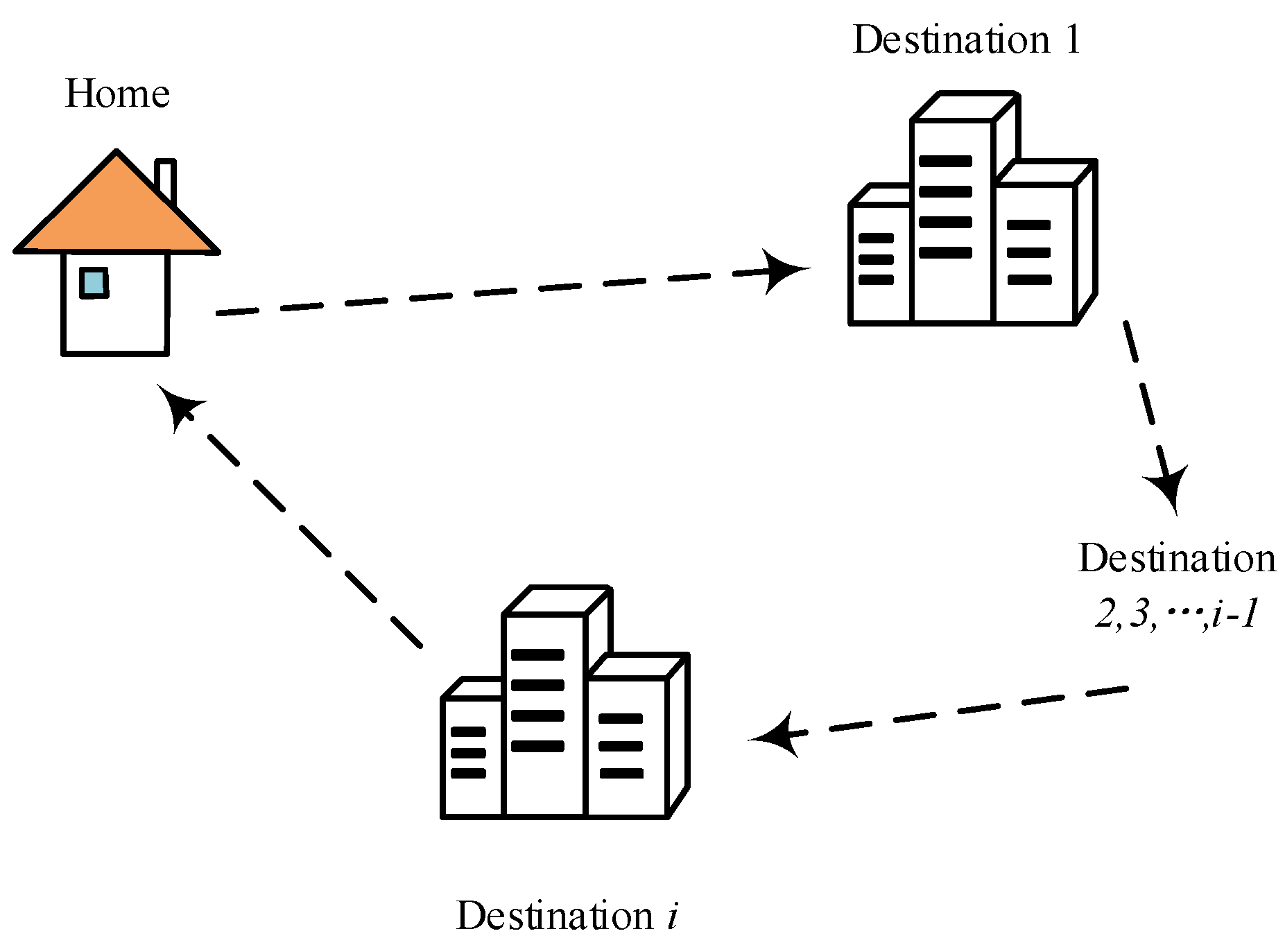
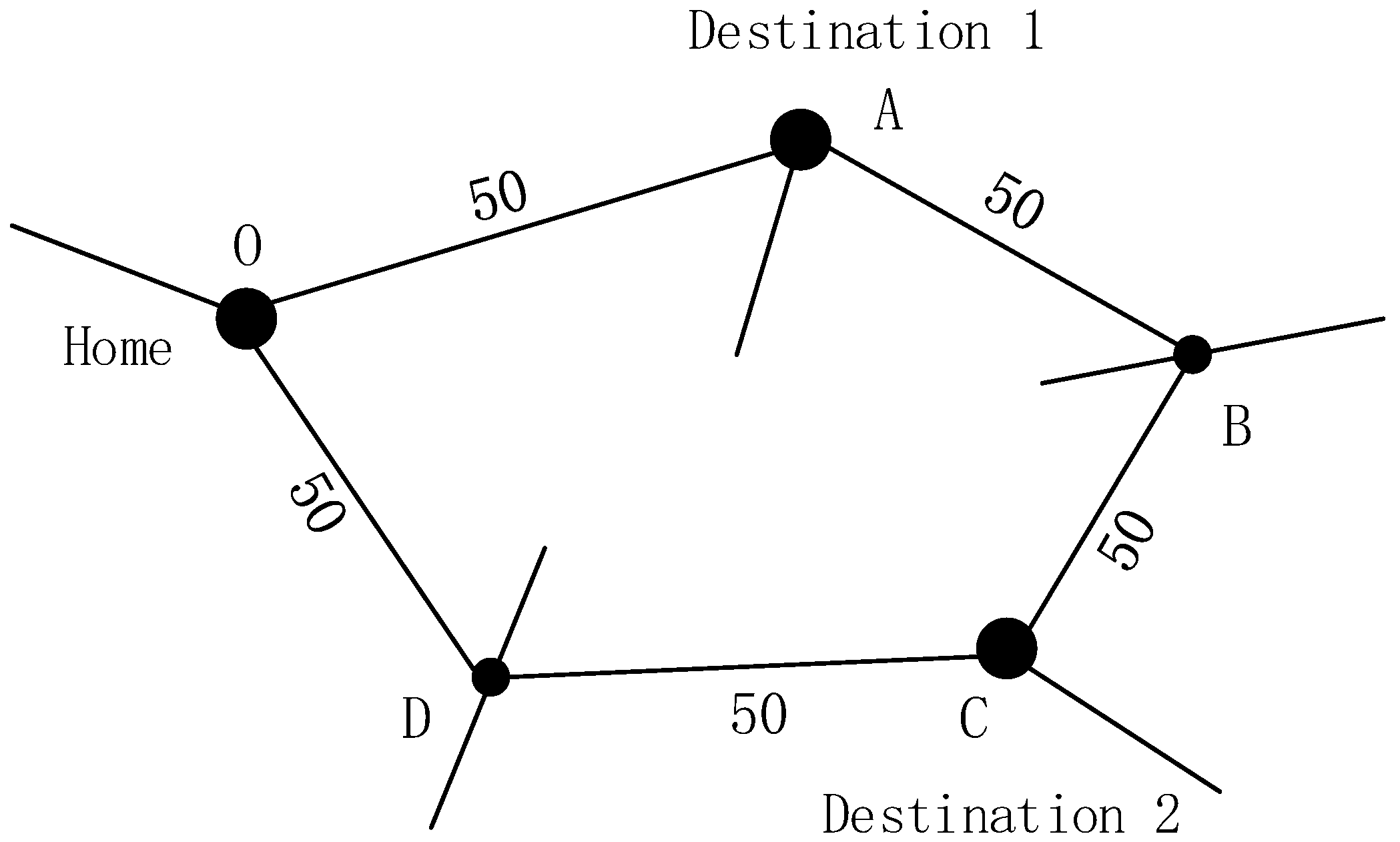
The following is a detailed introduction to the feasibility judgment method. Figure 5 illustrates the spatial characteristics for one route with two destinations (A and C), one original home node (O) and two common road nodes (B and D). Each path between nodes is the shortest path generated by Dijkstra’s algorithm, the total length of the whole route A-B-C-D-A is 250 miles. We will use this example to describe all the possible conditions that the user may encounter and the criteria for the feasibility of the route, as below.

Before the travel, we suppose all drivers have already determined the quantities and location of destinations on the day before the trip and planed the route in advance with the help of smart navigation apps such as Google Maps, which can provide the refueling station information that users may use on their way.

Case 1: If initial fuel tank level is over 250 miles, for example $ift{l}_i^p = 300$, there is no doubt that the car can go through all the journeys without refueling.

Case 2: If initial fuel tank level is below 250 miles and there is no refueling station available on the route. The vehicle cannot finish this closed loop journey, and we deem that this route plan is not successful. Users will need change their route to complete the planned trip tomorrow. In our model, although a user may plan a new route, the new route is not considered when calculating the total success radio.

Case3: If initial fuel tank level is below 250, for example $ift{l}_i^p=200$, and there are refueling stations on the route. The possible combinations of location for refueling station are {O}, {A}, {O,A}, {O,B}, {O,C}, {O,D}, {A,B}, {A,C}, {A,D}, {B,C}, {B,D}, {C,D}, {O,A,B}, {O,A,C}, {O,A,D},{O,B,C}, {O,B,D}, {O,C,D}, {A,B,C}, {A,B,D}, {A,C,D}, {B,C,D}, {O,A,B,C}, {O,A,B,D}, {O,B,C,D}, {A,B,C,D}, {O,A,B,C,D}, a total of 31 combinations. If we analyze each case one by one, the computational progress of calculation to determine whether it is successful is very complex and time-consuming. In fact, when the total path contains n nodes, the number of possibility combinations is $2^n-1$. When the number of nodes increases, the number of combinations increases exponentially, and the amount of calculation increases sharply. So we need to find a new way to judge the possibility to avoid computational complexity.

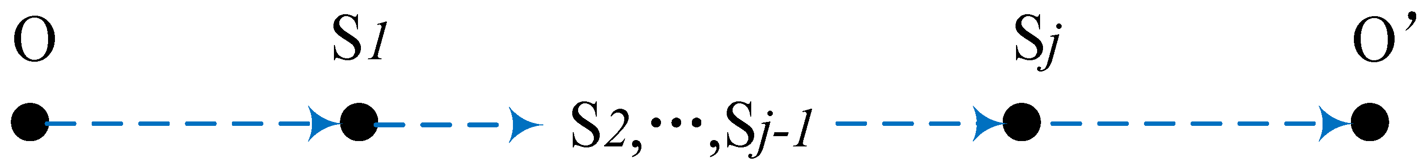
In fact, when the set of locations of the refueling stations is known, there is a quick way to judge whether this refueling station location combination can support vehicle to go through all the journeys. Figure 6 is a simplified schematic diagram of Case 3 where the destination node is omitted, $\mathrm{O}$ and $\mathrm{O}’$ are the same node which refer to the home location.

The route is deemed a success if and only if:

when $i=1$,

$$l_i(O,s_i^1)\geqq \zeta \times ift{l}_i^p$$

(1)

$$l_i(s_i^1,O’)\geqq {\mathsf{\lambda }\times \mathsf{\zeta }\times \mathrm{dr}}_i^p$$

(2)

when $i>1$,

$$l_i(O,s_i^1)\geqq \zeta \times ift{l}_i^p$$

(3)

$$l_i\left(s_i^{j-1},s_i^j\right)\geqq {\mathsf{\lambda }\times \mathsf{\zeta }\times \mathrm{dr}}_i^p$$

(4)

$$l_i\left(s_i^j,O’\right)\geqq {\mathsf{\lambda }\times \mathsf{\zeta }\times \mathrm{dr}}_i^p$$

(5)

where $i$ refers to route $i, j$ refers to refueling station $j$, $l_i\left(s_i^{j-1},s_i^j\right)$ refers to the shortest path length between station $s_i^{j-1}$ and $s_i^j$, $ift{l}_i^p$ refers to initial fuel tank level for route $i$, $\zeta$ refers to the safety threshold for tank below which driver will look for refueling station immediately, $\mathsf{\lambda }$ refers to drivers’ preference for refueling level at refueling station. ${\mathrm{dr}}_i^p$ refers to the driving range for p type vehicle i. It is important to notice that if there are destinations between $s_i^{j-1}$ and $s_i^j$, $l_i\left(s_i^{j-1},s_i^j\right)$ is not the shortest path length generated by Dijkstra’s algorithm, it should consider the path to and from destinations. Suppose there is one destination ${\mathrm{D}}_i^k$ between $s_i^{j-1}$ and $s_i^j$, $l_i\left(s_i^{j-1},s_i^j\right)$, we have:

$$l_i(s_i^{j-1},s_i^j)=d_i\left(s_i^{j-1},{\mathrm{D}}_i^k\right)+d_i\left({\mathrm{D}}_i^k,s_i^j\right)$$

(6)

where $d_i\left(s_i^{j-1},{\mathrm{D}}_i^k\right)$ represents the shortest path length via Dijkstra’s algorithm.

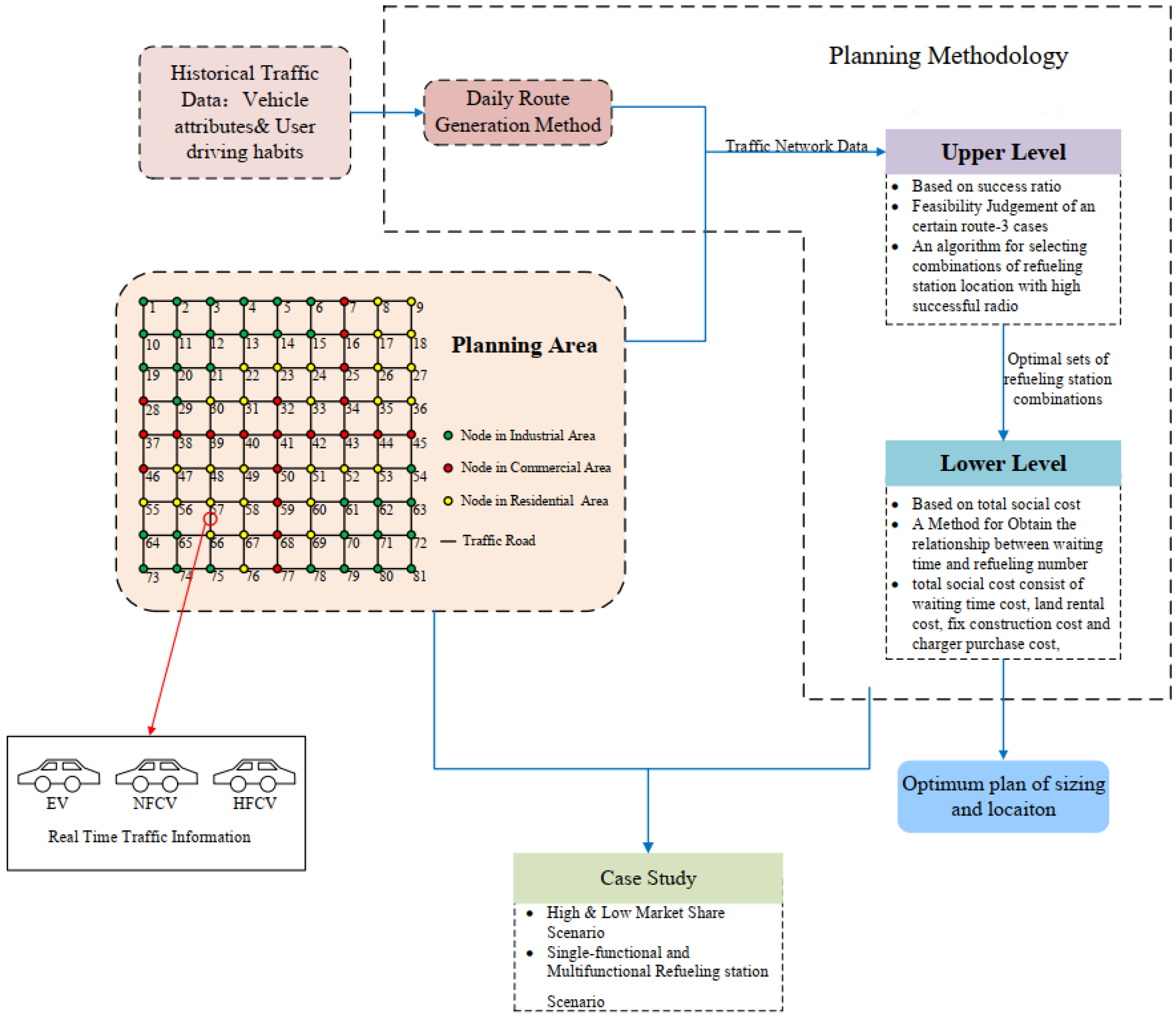
2.2.2. An Algorithm for Selecting Combinations of Refueling Station Location with High Success Ratio

The purpose of the upper model is to find a set of combination h of refueling station nodes which have a relatively high success ratio. With a great number of possible route plans generated by the method proposed in Section 2.1.2, an algorithm is necessary to determine which case (or cases) matches each route and selects the optimal combination of refueling stations based on the value of success ratio. Before implementing the algorithm, there is an unrealistic scenario if the algorithm is only based on the objective of maximum success ratio. The scenario is that the number of refueling station would be very large (located in every possible location for CS) according to the objective of achieving the highest success ratio. However, a large number of planned refueling stations is not economically friendly and achievable. We eliminated the negative outcome by the assumption that the government will limit the total number of refueling stations to maximal $\mathsf{\mu }$. The following steps are adopted to obtain the set of refueling station locations combinations with a relatively high success ratio.

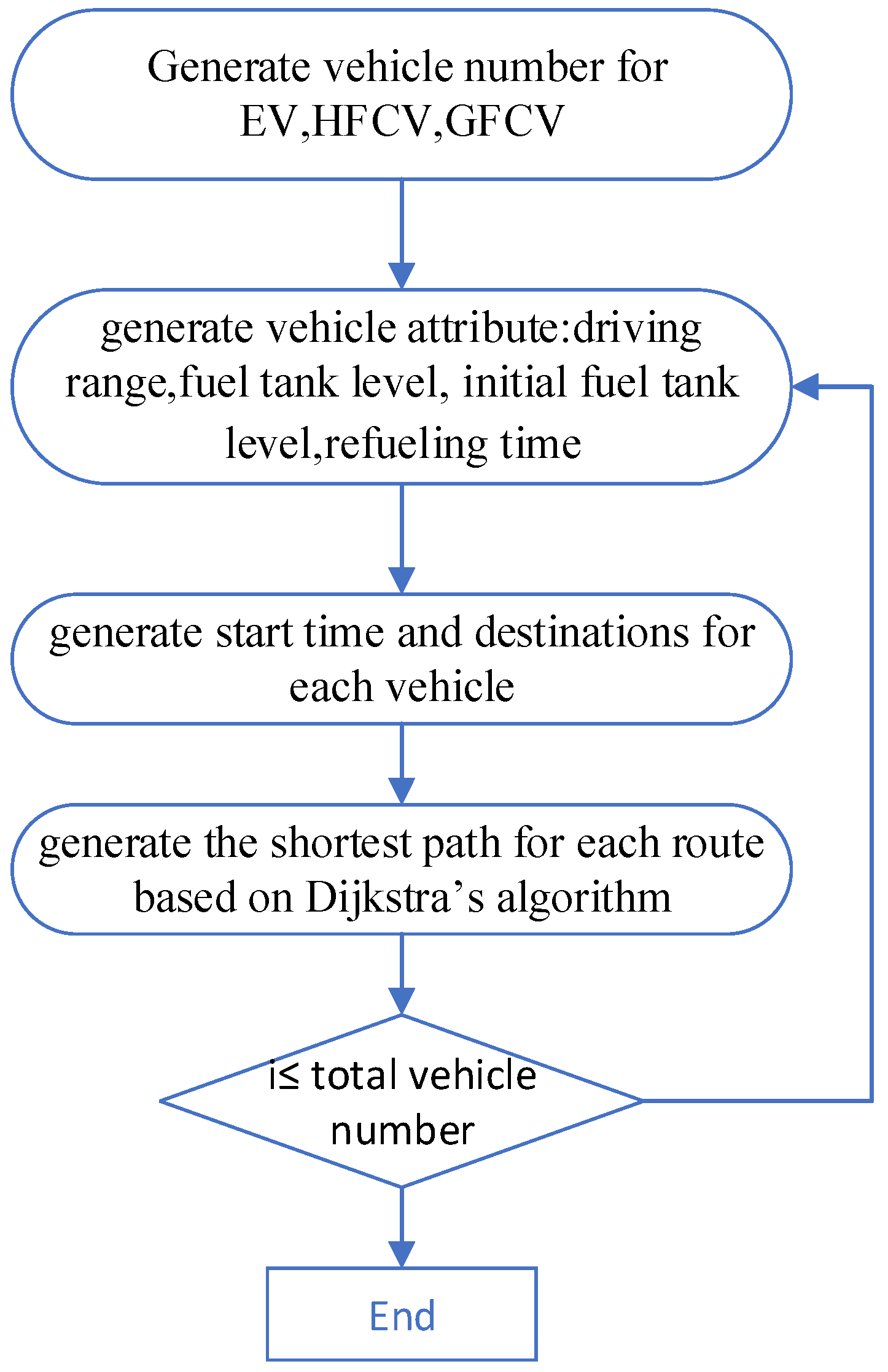
Step 1: Initialization based on a daily route generating method.

(1) Generate the daily route including number, location, type, and sequence of destinations, location of home, and shortest path for all cars, store the all the related nodes and links of paths.

(2) Establish and initialize an empty master list h, p, y and g.

Step 2: Beginning with the next route $i$, implement feasibility analysis, if case 1 is not suitable for route i, then it is necessary to generate all the possible combination of refueling stations.

(1) If initial fuel tank level is over total route length, this route is deemed to a success, record $s_i=1$ and jump to next route $i+1$, if not continue to the next step.

(2) Generate all the possible combinations of refueling stations, for example, for the route in Figure 3, the possible combinations are {O}, {A}, {O,A}, {O,B}, {O,C}, {O,D}, {A,B}, {A,C}, {A,D}, {B,C}, {B,D}, {C,D}, {O,A,B}, {O,A,C}, {O,A,D},{O,B,C}, {O,B,D}, {O,C,D}, {A,B,C}, {A,B,D}, {A,C,D}, {B,C,D}, {O,A,B,C}, {O,A,B,D}, {O,B,C,D}, {A,B,C,D}, {O,A,B,C,D}. Analyze the feasibility of each combination, store all the success combination in the master list h.

(3) Remove combinations that are supersets of any other remaining combinations in master list h.

(4) Repeat steps 2.1–2.3 for all the route i.

Step 3: Put all refueling stations involved in master list h, and generating all the subsets of master list h with elements less than $\mathsf{\mu }$, index each subset sequentially beginning with 1 and record all the subsets in master list p.

(1) Beginning with the next subsets j, record the feasibility outcome for each route i (${\mathrm{FJ}}_{ji}$ = 1 if success, ${\mathrm{FJ}}_{ji}=0$ if fail).

(2) Calculate the success ratio according to Equation (7), record it in master list y, jump to step 3.1 until there is no subset left.

$$s{r}_j=\frac{1}{n}{\displaystyle \sum }_{i=1}^n{s}_{ji}$$

(7)

where n refers to the total number of cars.

(3) Rank the success ratio list, and select the subsets with top 10% scores, record the subsets which include the number and locations of refueling stations and the associated success ratio into master list g.

After the whole progress, a list of optimal combinations of refueling station locations and corresponding success ratio value are obtained.

2.3. Lower-Level Mode

After running the upper model algorithm, a set of optimal solutions with a relatively high success ratio is obtained. However, the planning problem of refueling station in a certain area is not only to find the distribution of refueling station that capture most traffic flows. Economic factors and customer satisfaction also need to be taken into account when searching for an optimum solution. Therefore, we introduced the lower model to find the optimum solution considering economic factors and user satisfaction factor.

The purpose of lower model is to (1) select the optimum combination of refueling station location from master list h in term of user satisfaction index and total social cost, and (2) to determine the capacity of each refueling station.

2.3.1. A Method for Obtaining the Relationship Between Average Waiting Time and Charger Number

For a certain distribution plan of refueling stations in master list g, the time when vehicle i arrives at nodes $n_i^m$ is:

$${\mathrm{t}}_i^m=\frac{l(O,n_i^m)}{V}+S{T}_i+{\displaystyle \sum }_{k=1}^{d}S{D}_i^k$$

(8)

where node O refers to the origin node, $l(O,n_i^m)$ refers to the path length from node O to node $n_i^m$, i refers to route number which is the same as vehicle number, m refer to the node number in route i, $S{T}_i$ refers to the start time of vehicle i from home, ${\displaystyle \sum }_{k=1}^{d}S{D}_i^k$ refers to the total stay duration in destinations before arrive node $n_i^m$ based on the assumption that the user has been to d destinations before the node $n_i^m$. Note that Equation (8) does not consider refueling time and waiting time.

In this way, we obtained the timetable of each vehicle. For each refueling station, we recorded the arriving time of vehicle $i$ and summed it up to obtain the refueling demand during 24 h for each potential refueling station.

Nowadays, the communication system for traffic control has not been commonly used. Therefore, we assume that the mechanism of refueling service in station follows the ‘first come, first service’ rule. Based on this assumption, we introduced a simplified way to estimate the waiting time. First, select the busiest one-hour period from the refueling demand table for each refueling station. Suppose a total of n vehicles need to refuel, sort them by arrival time. Assume that the number of vehicles that need to be charged is always larger than the number of chargers during the busiest period, so that all the chargers are kept in service without rest. Then the waiting time can be estimated roughly from the number of chargers:

$$WT\approx \frac{A{T}_n+A{T}_1-\frac{{{\displaystyle \sum }}_1^{n}f{t}_i^p}{CN}}{n}$$

(9)

where $WT$ refers to waiting time, $A{T}_1$ refers to the arrive time for the first arrive vehicle, ${\displaystyle \sum }_1^{m}f{t}_i^p$ refers to the total refueling time for vehicle 1 to m, $A{T}_1$ refers to the arrive time for the last arrive vehicle, $f{t}_m^p$ refers to refueling time of the last arrive vehicle (vehicle n), $CN$ refers to the total number of chargers. Noted that Equation (9) is only accurate when the fueling demand is high.

2.3.2. Total Social Cost

The total social cost consists of waiting time cost, land rental cost, fix construction cost, and charger purchase cost, the total social cost is shown as Equation (10):

$$C={\displaystyle \sum }_{h=1}^H(W{T}_h\times M_h\times C_{tc})+{\displaystyle \sum }_{h=1}^H(C_{fc,h}+L_h{C}_{lc,h}+C_{cc,h})$$

(10)

where ${\displaystyle \sum }_{h=1}^H(W{T}_h*M_h*C_{tc})$ refers to the total waiting time cost of users, H refers to the total number of refueling stations, $W{T}_h$ refers to the waiting time in refueling station h, $M_h$ refers to the total customers number in refueling station h during the busiest period, $C_m$ is the time cost of each user, ${\displaystyle \sum }_{h=1}^H(C_{fc,h}+L_h{C}_{lc,h}+C_{cc,h})$ refers to the investment cost including land rental cost $(L_h{C}_{lc,h})$, fix construction cost (C_fc,h) and charger purchase cost ($C_{cc,h}$).

Assume that the total number of chargers in reality is 20% larger than the number of chargers calculated by our model, that is:

$$C_{cc,h}=1.2\times {\displaystyle \sum }C{N}_p$$

(11)

where $C{N}_p$ refers to the charger number for vehicle of p kind.

2.3.3. Mathematical Model

The mathematical model for lower level model considering the success ratio given by the upper model can be described as:

$$\mathrm{Min}f=C+\xi \times sr$$

(12)

Subject to Equations (9)–(11).

where $f=C+\xi \times sr$ is the objective function, $\xi \times sr$ represents the success ratio factor when considering the optimal solution, $\xi$ is the coefficient for the success ratio. C refers to the total social cost of the whole area.

Finally, we used Gurobi Software to solve this mixed integer optimization problem in Python 2.7. The proposed model is a (Mix Interger Linear Problem) MILP problem, and there is no high-dimensional nonlinear nonconvex optimization problem. It can be solved by using software like GUROBI, CPLEX, and other solvers. We used the Python interface of GUROBI to call GUROBI to solve the problem. A similar MILP problem to that solved by GUROBI can be found in other research [24].

3. Results and Discussion

3.1. Planning Area

Figure 7 shows a simplified city map with an area of $45\times 45{\mathrm{km}}^2$. The planning city area is split by three functional zones: industrial zone, commercial zone, and residential zone. Like the structure of typical medium-sized and large-sized cities, the commercial area is in the city center, the industrial area is on the edge of the city because the land price is cheap, and the residential area is distributed between the commercial area and the industrial area. Our model is based on the assumption that all refueling station are distributed at traffic nodes. We do not consider the midlink location as a potential location because the benefits of a refueling station in the midlink location may be offset by the fact that it is unable to refuel the crossing traffic flows [2]. There are a total of 81 traffic nodes in our model, among which, commercial area has 20 traffic nodes, residential area has 29 traffic nodes, and industrial area has 32 traffic nodes.

Table 3. Model Parameters.

Parameter	Value
$\zeta$	5%
$\mathsf{\lambda }$	80%

shows the parameters used in our model, most of the value is hypothetical.

Table 4. Land Rental Cost for three functional zones [13].

Area Type	Residential Area	Industrial Area	Commercial Area
Land Rental Cost ($\$/{\mathrm{m}}^2$)	330	109	1070

shows the land rental cost in different functional zones.

3.2. Low-Emission Vehicles (LEVs) Vehicle Market Share Scenarios Based on Multifunctional Refueling Stations

In this part, we evaluate the impact of LEVs vehicles penetration on the optimal location of refueling station. Before the analysis, we assume that the number of BEVs, HFCVs, and GFCVs in the planning area are identical, 1000 per type in low penetration situation and 4000 per type in high penetration situation. That is, the total number of LEVs vehicle is 3000 in low penetration case, and 12,000 in high penetration situation. Assume that the city’s land planning department allows up to 10 refueling stations to be established due to policy and economic factors. Bring this factor into the upper model and obtain a set of optimal location combinations for 10 cases where the total number of refueling station is 1 to 10. After that, the most optimal combination of refueling stations and number of chargers for each station are determined by lower models considering the total social cost and success ratio. Figure 8a,b reveals that the relationship between success ratio and total number of refueling stations is positively related. However, along with the number of refueling stations increases, the convergence gap becomes smaller. The growth rate of success ratio in high penetration situation is higher than that in the low penetration situation. Figure 8c,d displays the traffic flow information in term of arrive frequency. Compared with optimal location shown in

Table 5. The optimum plan for low and high market share scenarios.

Traffic Type	Total Number of Refueling Stations	Successful Ratio	Optimal Location	Number of Chargers in Each Station
Low Penetration	5	81%	32, 40, 41, 49, 51	14, 18, 16, 17, 13
High Penetration	7	88%	23, 24, 40, 41, 48, 52, 60	33, 34, 48, 41, 34, 30, 32

, we find that most of traffic nodes which are selected as a refueling station by lower models have high arrival frequency. Figure 8e,f illustrate the changes of total investment along with the change of total number of refueling stations from 1 to 10, the optimum number of refueling station is 5 for low market share scenario and 7 for high market scenario as the objective function f is smallest. Figure 8g,h shows that average waiting time drops fast in both scenarios as the refueling station number increases, for the optimum result determined by the lower model, the average waiting time in high penetration (4.34 min) is nearly half of that in low penetration (7.27 min). Therefore, high market share of LEVs vehicle can greatly reduce the average waiting time in our model. Figure 9 summarizes the geographical distribution of refueling station in low and high market share scenarios. Although industrial land accounts for 40% of a proposed city, the optimum results calculated by our model suggests that it is unnecessary to invest in a refueling station in industrial areas. Furthermore, we collect the refueling frequency data for BEV, HFCV, and GFCV. According to the data, it can also be found that there are 78.67% BEV, 25% HFCV, and 3% GFCV who can finish their journey without refueling. Those numbers are related closely to the initial fuel tank level when drivers start at home. Because the penetration of household chargers for BEV is absolutely high than that for HFCV, GFCV, so most of BEV can complete their daily route without refueling because their 100% initial battery level can cover the whole route. At the beginning of simulation, we assumed that the initial fuel tank level for all BEVs are 100% while that of HFCV and GFV are 50%. The result is reasonable. The data also indicated that most of the daily route in city is below 200 miles.

3.3. Single-Functional and Multifunctional Refueling Station Scenarios

Nowadays, refueling stations service for different types of LEVs vehicle are usually constructed as single function. This section is to study the possibility of replacing single-functional refueling station by MFCS. Planning method for single functional refueling station is similar to the method of MFCS planning. Firstly, the vehicle number for each type is assumed to be 1000 (total number is 3000, same as that in low penetration scenario using multifunctional refueling station), and then generate daily routes for BEV, HFCV, and GFCV based on the method in Section 2, bring the traffic data into the proposed bi-level model respectively. If BEV, HFCV, and GFCV need refueling stations in the same location, we combine them into a multifunctional refueling station and use ‘EHG’ represent it, as well as ‘GE’ and ‘GH’. ‘EHG’ refers to the stations that service BEV, HFCV, and GFCV, ‘GH’ refers to the stations that service HFCV and GFCV, ‘GE’ refers to the stations that service BEV and GFCV. The optimum results are shown in Figure 10.

Because vehicles have the fuel anxiety value which means it can travel a limited distance before the defined unsuccessful fuel tank level when a vehicle needs to refuel, it can detour to the near station for refueling. Thus, we can combine every two single functional refueling station if the distance between them is shorter than 10 miles (assume the fuel anxiety value is 5%). Therefore, the optimum location of refueling station after adjustment is shown in Figure 10.

Table 6. The outcome between single-functional and multifunctional refueling station.

Refueling Station Type	$\mathbf{Objective}\mathbf{Function}\mathbf{f}(\times \$103)$	$\mathbf{Investment}\mathbf{Cos}\mathbf{t}(\times \$103)$	$\mathbf{Waiting}\mathbf{Time}\mathbf{Cos}\mathbf{t}(\times \$103)$	Land Rental Cost	Charger Cost	Average Waiting Time (Minute)
Single-Functional Refueling Station	314.8	1986.33	21.63	980	124.6	11.21
Multifunctional Refueling Station	740.3	1503.2	6.2	360	52.7	7.27

shows the cost comparison between single-functional refueling station and multifunctional refueling station based on our model in low penetration scenario. From Table 6, we conclude that MFCS is better than single functional refueling station in term of investment cost, waiting time cost, land rental cost, charger purchase cost, and average waiting time. Due to the success ratio for using the single functional station method being very high, the value of objective function f of single functional refueling station is relatively low. However, this benefit may be offset by the fact that 20 refueling stations are needed if we construct single-functional station independently while only 7 refueling station are needed in the MFCS scenario. Besides, almost 72% of refueling action for HFCV happens upon returning to home.

4. Conclusions

In this article, we introduced a methodology for the optimal planning of MFCSs which are able to serve multi-types vehicles (BEV, HFCV, GFCV). We verified the proposed planning methodology in a medium-sized city with 81 simplified traffic nodes. For most of the existing literature regarding the location and sizing problem of LEVs, vehicles are generally assumed to have the same attributes which is impossible in reality. To reflect the actual traffic flow in urban area, we defined four attributes (driving range, initial fuel tank level, current fuel tank level, and refueling time) to distinguish vehicles that use different fuel types (electric, hydrogen fuel cell, and natural gas). In order to figure out the daily travel route for drivers, we introduced a multi destination method. Usually, the daily route for each user is a closed-loop journey which starts and ends at home. The lifestyle of users who live in the city is not easy to predict, however, the possibility of going to every possible destination is concluded by surveys. Surveys also suggest the relationship between start time and destination types. Therefore, the daily route data for the whole city can be generated by the data mentioned before based on the Monte Carlo simulation.

In order to solve this multi-objective question effectively, we divided the model into two sub-models. The purpose of upper model is to select a number of optimal plans of refueling station locations based on the max-cover ratio (success ratio). We proposed a judgment method for the feasibility of the travel route, and explain it by a simple example. After that, an algorithm for selecting optimal combinations of refueling station location with high success ratio was established. Considering the investment budget, we selected every optimum plan for different situations where the total number of refueling station is from one to ten. These data will be put into the lower model.

The purpose of the lower model is to select the optimum plan from the optimal results given by the upper model. The determining factors includes not only successful ratio, but also the investment cost (charger purchase cost, fix construction cost and land rental cost) and waiting time cost. We simplify the relationship between waiting time and charger number in the busy period, and consider it as a constraint when solving lower model optimal questions.

We verified the model in two directions (1) how low and high LEVs vehicle market share will impact the planning of refueling stations; (2) comparison of single-functional refueling station and multifunctional refueling station in the planning progress. The main conclusions are listed as follows:

For a middle-sized city, the number of refueling station is suggested to be 5 (with 81% success ratio) for low LEV market share scenario and 7 (with 88% success ratio) for high LEV market share scenario. It is suggested that all of refueling stations are distributed in residential areas and commercial area and no refueling station is needed in industrial area although it accounts for 40% land. With the increase of market share, the distribution of refueling stations is gradually shifting to residential areas (from 40% to 70%).

The proposed location and sizing model performs better in a high LEV market share scenario. After a 300% increase in vehicles, the construction cost only increased by 44.8%, but the average waiting time decreased by 40.3%, and the success ratio increased from 81% to 88%.

The transformation to multifunctional refueling station from single-functional refueling station is possible and positive. For a medium-sized city, the number of multifunctional refueling stations needed to achieve 88% success rate is 7 while the number of single-functional refueling stations needed in the same situation is 20. The reduction in the number of refueling stations directly reduced the cost of land to 36.73% of the single-functional refueling station scenario. Besides, multifunctional refueling station greatly reduce the average waiting time by 35%.

Future research will center on the planning method when a vehicle is allow to detour when finding a refueling station.

References

1. Hosseini, M.; Dincer, I.; Ozbilen, A. Expert Opinions on Natural Gas Vehicles Research Needs for Energy Policy Development. Exergetic Energetic Environ. Dimens. 2018, 731–750. [Google Scholar] [CrossRef]
2. Ally, J.; Pryor, T. Life-cycle assessment of diesel, natural gas and hydrogen fuel cell bus transportation systems. J. Power Sources 2007, 170, 401–411. [Google Scholar] [CrossRef] [Green Version]
3. Upchurch, C.; Kuby, M.; Lim, S. A Model for Location of Capacitated Alternative-Fuel Stations. Geogr. Anal. 2009, 41, 85–106. [Google Scholar] [CrossRef]
4. Dharmakeerthi, C.H.; Mithulananthan, N.; Saha, T.K. Modeling and planning of EV fast charging station in power grid. In Proceedings of the 2012 IEEE Power and Energy Society General Meeting, San Diego, CA, USA, 22–26 July 2012; pp. 1–8. [Google Scholar]
5. Dong, X.; Mu, Y.; Jia, H.; Wu, J.; Yu, X. Planning of Fast EV Charging Stations on a Round Freeway. IEEE Trans. Sustain. Energy 2016, 7, 1452–1461. [Google Scholar] [CrossRef]
6. Frade, I.; Ribeiro, A.; Gonçalves, G.; Antunes, A.P. Optimal Location of Charging Stations for Electric Vehicles in a Neighborhood in Lisbon, Portugal. Transp. Res. Rec. J. Transp. Res. Board 2011, 2252, 91–98. [Google Scholar] [CrossRef] [Green Version]
7. Andrenacci, N.; Ragona, R.; Valenti, G. A demand-side approach to the optimal deployment of electric vehicle charging stations in metropolitan areas. Appl. Energy 2016, 182, 39–46. [Google Scholar] [CrossRef]
8. Wang, G.; Xu, Z.; Wen, F.; Wong, K.P. Traffic-Constrained Multiobjective Planning of Electric-Vehicle Charging Stations. IEEE Trans. Power Deliv. 2013, 28, 2363–2372. [Google Scholar] [CrossRef]
9. Zang, H.; Fu, Y.; Chen, M.; Shen, H.; Miao, L.; Zhang, S.; Wei, Z.; Sun, G. Bi-Level Planning Model of Charging Stations Considering the Coupling Relationship between Charging Stations and Travel Route. Appl. Sci. 2018, 8, 1130. [Google Scholar] [CrossRef] [Green Version]
10. Huang, Y.; Li, S.; Qian, Z.S. Optimal Deployment of Alternative Fueling Stations on Transportation Networks Considering Deviation Paths. Netw. Spat. Econ. 2015, 15, 183–204. [Google Scholar] [CrossRef]
11. Nie, Y.; Ghamami, M. A corridor-centric approach to planning electric vehicle charging infrastructure. Transp. Res. Part B Methodol. 2013, 57, 172–190. [Google Scholar] [CrossRef]
12. Kuby, M.; Lim, S. The flow-refueling location problem for alternative-fuel vehicles. Socio-Econ. Plan. Sci. 2005, 39, 125–145. [Google Scholar] [CrossRef]
13. Lim, S.; Kuby, M. Heuristic algorithms for siting alternative-fuel stations using the Flow-Refueling Location Model. Eur. J. Oper. Res. 2010, 204, 51–61. [Google Scholar] [CrossRef]
14. MirHassani, S.A.; Ebrazi, R. A Flexible Reformulation of the Refueling Station Location Problem. Transp. Sci. 2013, 47, 617–628. [Google Scholar] [CrossRef]
15. Awasthi, A.; Venkitusamy, K.; Padmanaban, S.; Selvamuthukumaran, R.; Blaabjerg, F.; Singh, A.K. Optimal planning of electric vehicle charging station at the distribution system using hybrid optimization algorithm. Energy 2017, 133, 70–78. [Google Scholar] [CrossRef]
16. Chung, S.H.; Kwon, C. Multi-period planning for electric car charging station locations: A case of Korean Expressways. Eur. J. Oper. Res. 2015, 242, 677–687. [Google Scholar] [CrossRef]
17. Zhang, H.; Hu, Z.; Xu, Z.; Song, Y. An Integrated Planning Framework for Different Types of PEV Charging Facilities in Urban Area. IEEE Trans. Smart Grid 2015, 7, 1. [Google Scholar] [CrossRef]
18. Oda, T.; Aziz, M.; Mitani, T.; Watanabe, Y.; Kashiwagi, T. Mitigation of congestion related to quick charging of electric vehicles based on waiting time and cost–benefit analyses: A japanese case study. Sustain. Cities Soc. 2018, 36, 99–106. [Google Scholar] [CrossRef]
19. Gu, W.; Zhuang, Y.; Gu, W.; Wu, Z. Operation and Economic Assessment of Hybrid Refueling Station Considering Traffic Flow Information. Energies 2018, 11, 1991. [Google Scholar]
20. Hwang, S.W.; Kweon, S.J.; Ventura, J.A. Locating alternative-fuel refueling stations on a multi-class vehicle transportation network. Eur. J. Oper. Res. 2017, 261, 941–957. [Google Scholar] [CrossRef]
21. Ghamami, M. Electric Vehicle Charger Placement Optimization in Michigan: Phase I-Highways; Technical Report; Michigan State University: East Lansing, MI, USA, 2019. [Google Scholar]
22. Pod-point.com. How Long Does It Take to Charge an Electric Car?|Pod Point. Available online: https://pod-point.com/guides/driver/how-long-to-charge-an-electric-car (accessed on 22 August 2019).
23. Fueleconomy.gov. Compare Fuel Cell Vehicles. Available online: https://nhts.ornl.gov/assets/2017_nhts_summary_travel_trends.pdf (accessed on 22 August 2019).
24. Nguyen, V.H.; Tuong, N.H.; Tran, V.H.; Thoai, N. An MILP-based Makespan Minimization Model for Single-machine Scheduling Problem with Splitable Jobs and Availability Constraints. In Proceedings of the 2013 International Conference on Computing, Management and Telecommunications (ComManTel), Ho Chi Minh City, Vietnam, 21–24 January 2013; pp. 397–400. [Google Scholar]
Figure 1. The overall schematic diagram of the whole paper.
Energies 13 01283 g001
Figure 2. The schematic diagram of a closed loop vehicle route.
Energies 13 01283 g002
Figure 3. Distribution of Private Vehicle Trips Percent by Start Time and Trip Destination type [23].
Energies 13 01283 g003
Figure 4. The Flowchart for Generating the Route Data.
Energies 13 01283 g004
Figure 5. Example closed loop trip flow for one vehicle’s route.
Energies 13 01283 g005
Figure 6. Simplified Schematic Diagram of Case 3.
Energies 13 01283 g006
Figure 7. The schematic diagram of Planning Area.
Energies 13 01283 g007
Figure 8. The Numerical Outcome for Low and High Market Share.
Energies 13 01283 g008
Figure 9. The Distribution of Refueling Station in Low and High Penetration Scenario.
Energies 13 01283 g009
Figure 10. The optimal location for single-functional and multifunctional refueling stations.
Energies 13 01283 g010