Abstract
The success of electric vehicles (EVs) depends principally on their energy storage system. Lithium-ion batteries currently feature the ideal properties to fulfil the wide range of prerequisites specific to electric vehicles. Meanwhile, the precise estimation of batteries’ state of health (SoH) should be available to provide the optimal performance of EVs. This study attempts to propose a precise, real-time method to estimate lithium-ion state of health when it operates in a realistic driving condition in the presence of dynamic stress factors. To this end, a real-life driving profile was simulated based on highly dynamic worldwide harmonized light vehicle test cycle load profiles. Afterward, various features will be extracted from voltage data and they will be scored based on prognostic metrics to select diagnostic features which can conveniently identify battery degradation. Lastly, an ensemble learning model was developed to capture the correlation of diagnostic features and battery’s state of health (SoH). The result illustrates that the proposed method has the potential to estimate the SoH of battery cells aged under a distinct depth of discharge and current profile with a maximum error of 1%. This confirms the robustness of the developed approach. The proposed method has the capability of implementing in battery management systems due to many reasons; firstly, it is tested and validated based on the data which are equal to the real-life driving operation of an electric vehicle. Secondly, it has high accuracy and precision, and a low computational cost. Finally, it can estimate the SoH of battery cells with different aging patterns.
1. Introduction
Lithium-ion (Li-ion) batteries currently possess prominent attributes including low cost, high energy density, high power capability, low self- discharge and long lifetime, which can satisfy the requirements of energy storage systems (ESS) in electric vehicles [1]. Nevertheless, deterioration of lithium-ion batteries is inevitable phenomena due to various reasons such as solid electrolyte interphase (SEI) formation, lithium plating, or changes in active material [2]. Therefore, assessing the state of health (SoH) is crucial to guaranty the availability, safety, and reliability of Li-ion batteries. SoH is the ability of a battery cell to store energy relative to its initial value. It is considered a convenient criterion to understand battery degradation or detect a possible failure. A 100% percent value of SoH means the battery is fresh while decreasing SoH to 80% the battery cannot satisfy the requirements of electric vehicles (EVs) [3]. Investigations regarding developing SoH estimation methods have dominated research in recent years. SoH estimation methods are primarily classified into model-based and data-driven approaches. Model-based approaches develop an electrochemical or electrical model of battery to identify the state of batteries. These techniques characterize battery parameters by applying the adaptive filters such as particle filters [4] and Kalman filters [5]. Model-based methods are solid however, they require comprehensive domain knowledge and their development is time-consuming and complex [6]. Data-driven SoH estimation methods require an extensive volume of historical data to track battery degradation, nevertheless, they have gained much importance in recent years due to their simplicity and being model-free [7]. Sample entropy, statistical methods and machine learning (ML) are examples of data-driven methods. A recent study has thoroughly reviewed the data-driven methods for SoH estimation [8]. The framework of data-driven SoH estimation generally includes three main steps: (1) acquiring data (2) exploring historical data such as current, voltage and temperature to extract promising features [9] (3) feeding the features to a machine learning model to capture the correspondence between battery SoH and extracted features. Among these steps, the features extraction step is of utmost importance [10] since the accuracy of SoH estimation largely depends on the features that express distinct trends as battery degrades. These features called diagnostic features. Diagnostic features can be any feature that conveniently distinguishes battery deterioration from the beginning of life (BOL) to the end of life (EOL) different stages of battery aging. Prior studies addressed different diagnostic features for SoH estimation. Taking as an example, Guo et al. [11] extracted 14 diagnostic features from charging curve to describe the degradation of battery cell. They divided these featured into four groups which correspond to capacity, the ratio of constant current (CC) time to constant voltage (CV), temperature and current/voltage drop at CV and CC stage. The diagnostic features then used as input data for RVM model to predict SoH. Jian Liu and Ziqiang Chen [12] also considered the charge time interval of voltage varying from 3.9 V to 4.2 V; the charge voltage varying from 3.9 V to the voltage after 500 s and the CV charge current drop between 1.5 A (the CC charge current) and the current after 1000 s as three diagnostic features. They proposed to feed the diagnostic features into GPR model to predict remaining useful life lithium-ion batteries. Similarly, Deng et al. extracted four Diagnostic features from charging process and used them as SVM training data set to estimate SoH [13]. Some authors also proposed DFs by applying Incremental capacity (IC) and differential analysis. The advantage of IC analysis is that they can be applied on the partially charging data. For instance, Li et al. [14] established a correlation between SoH and features such as peaks and valleys detected on IC curves. Similarly, Weng et al. [15] investigated IC curves to extract the feature which are able to predict capacity fade. Aforementioned studies explored the diagnostic features under predefined conditions such as specific range of current or voltage and they need constant current charge and discharge cycling. However, battery cells which are used in automotive applications never operate under static conditions, yet, little studies have been conducted to evaluate SoH estimation under dynamic stress factors. Consequently, this research attempt to extract diagnostic features from the battery cells which operate in realistic condition. There are various standardized driving cycles that can be applied to imitate the real operation of an EV such as urban dynamometer driving schedule (UDDS), new European driving cycle (NEDC), and, worldwide harmonized light vehicles test (WLTC). Prior research generally confirms that WLTC profile satisfies the prerequisite of a realistic driving condition for an EV [16]. Therefore, our paper also uses the same profile as this research.
As mentioned earlier, the third step in the framework of data-driven SoH estimation is selecting a model for SoH estimation. Among all data-driven models, ML techniques particularly have appealed to diagnose battery health. ML methods can be considered as non-probabilistic such as artificial neural networks (ANN) [17] and support vector machine (SVM) and probabilistic methods including Gaussian process regression (GPR) [18] and relevant vector machine (RVM). Despite the convenient achievements of traditional ML methods in SoH estimation, they may not succeed in the context of noisy, nonlinear and complex data. Recently, ensemble learning algorithms are introduced to overcome the inefficiency of traditional ML methods. These algorithms have appealed to many researchers in different fields of research such as traffic prediction [19], engine health prediction [20], and battery state of charge estimation [21], owing to their effectiveness in prediction. The output of an ensemble algorithm is achieved by merging the base learners’ outputs [22]. Any kind of ML techniques such as ANN and decision tree can be considered as the base learner [23]. Integrating the prediction results of multiple base learners, an ensemble learning algorithm can considerably enhance the performance of the predictive model. The main reason is that by combination of multiple learners, the poor performance of an individual learner will likely be compensated by the rest of learners. Moreover, lack of training data causes that the prediction model can’t generalize from training data to untrained data. However, by averaging several hypotheses the risk of selecting the nonoptimal hypothesis can be reduced [24]. As a result, the prediction performance will be improved. In this study, one of the ensemble learning methods called gradient boosted tree (GBT) is proposed to estimate SoH. GBT is a powerful estimation model particularly in terms of robustness and dealing with nonlinearity. Despite these advantages, to the best of authors’ knowledge, few has utilized GBT for SoH estimation in lithium batteries. To fill this gap, present study attempts to employ this method for SoH estimation.
The remaining part of this paper is organized as follows; Section 2 introduces the proposed framework for SoH estimation. In this section experimental data, feature engineering and GBT model will be discussed in detail. Section 3 will focus on the analysis of the experimental results the efficiency of GBT will be also discussed in this section. Lastly, a concluding summary will be presented in Section 4.
2. Proposed SoH Estimation’s Framework
The proposed framework is divided into two phases: offline phase and an online phase. The entire framework is depicted in Figure 1. As Figure 1 presents the offline phase includes importing historical data, preparing data, feature engineering and developing a ML algorithm to capture the relation between features and SoH. The first step in the offline phase is importing pre-collected static data. Battery aging is characterized by different types of data such as voltage, current, capacity and temperature. In this study, voltage signal is selected as the experimental data since it is directly measurable by the battery management system (BMS), and many time-domain and frequency-domain features can be easily extracted from voltage signal. In the data preparation step, further processes are applied to data such as outlier removal, resampling and filtering. The feature engineering step includes feature exploration and evaluating their impact on battery degradation characterization based on prognostic metrics. The output of this step is a dataset of diagnostic features. An ensemble learning algorithm is trained and validated in the last step of offline phase. Feature engineering and training the algorithm steps are time-consuming and are not applicable in the online phase due to time constraints in real-time applications. In the online phase, real-time data which are imported from sensors are used. After processing sensor data, diagnostic features which are specified in the offline phase are extracted and are fed to the trained model to estimate SoH.
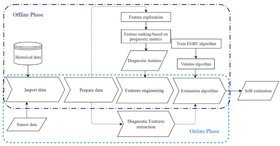
Figure 1.
Framework of SoH estimation
2.1. Experimental Data
The experiments were conducted using three nickel manganese cobalt oxide (NMC) pouch cells. NMC martial provides thermal stability during abuse and the raw materials costs are relatively low [25]. The nominal capacity and nominal voltage of all cells are 20 and 3.65 respectively, and the voltage operation range is 3 to 4.2 . The specification of tested cells is summarized in Table 1.

Table 1.
Specifications of tested cells.
The cells were cycled using WLTC profile under various conditions due to its similarity with an EV operation condition [16]. The driving profile represents both urban driving and suburban driving condition. During urban driving conditions, 6.75 km was traveled in 15 min and the average and maximum speed are 27 and 76.6 km/h respectively. However, a longer distance (16.51) was traveled in suburban driving conditions with the average and maximum speed of 66 and 131.3 km/h. WLTC’s current profile is depicted in Figure 2.
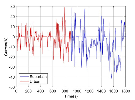
Figure 2.
Illustration of worldwide harmonized light vehicles test (WLTC) current profile. The first part considered being demonstrative of urban driving conditions while the second part simulates driving conditions in the suburban. Each section takes 15 min.
The experiment for Cell One conducted based on six full charge-discharge cycles each day. Each cycle consists of five successive WLTC trips that simulate both urban and suburban driving conditions. While solely suburban driving condition was applied for Cell Two and each full charge and discharge cycle includes four WLTC trips. Moreover, compared to Cell One, a lower rate of depth of discharge (DoD) and higher SoC window was applied. Figure 3 demonstrates the voltage signal for Cells One and Two gathered in one day of the experiment.
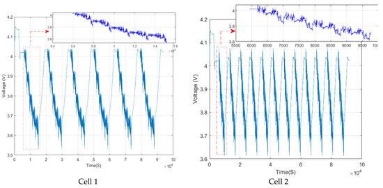
Figure 3.
Recorded voltage data in one day of experiment for Cell One and Two.
The experiment conditions for Cell Three are similar to Cell One except that Cell Three was tested at different temperature. The cells are cycled under the conditions which are summarized in Table 2.
Table 2.
Cell aging test conditions.
A capacity test was performed at the BOL to identify the initial capacity and after particular numbers of cycling a capacity checkup was conducted using constant current-constant voltage (CC-CV) protocol with a C-rate of C/2 in the charging and discharging steps to identify capacity loss. The SoH is then calculated according to Equation (1).
where is the recorded discharge capacity obtained from capacity checkup test and is the initial capacity.
2.2. Data Preparation
Collected raw data are not convenient for feature engineering. Data preparation implies to transfer collected data into interpretable and exploitable knowledge. In this step, the principal focus is to remove outlier, resample, decimation, detrend and eliminating direct current (DC) component from raw voltage. The signal analyzer and filter designer applications provided by MATLAB are used to perform data preparation. These applications help to remove the outlier, interpolate non-uniform data without introducing misidentification or aliasing of a signal frequency. Moreover, to eliminate the DC component, a bass-cut filter was developed using filter designer application. By removing DC component, the signal pattern is more likely to be identified clearly and it is useful for revealing descriptive features.
2.3. Feature Engineering
In this study, feature engineering implies the process of identifying features which are proper to describe aging pattern. As mentioned before, the output of this stage is a set of diagnostic features. Diagnostic features express predictable trends during the trajectory of battery life. Therefore, they can considerably improve the accuracy and performance of SoH estimation model. Feature exploration together with feature selection constitute feature engineering stage. The feature exploration step includes analyzing of voltage data to extract a set of a dataset of features. The features are extracted using signal processing techniques. However, the extracted features should be evaluated in the feature selection step to determine if the features are potentially convenient for SoH estimation. Features exploration and feature selection steps will be discussed in detail in Section 2.3.1 and Section 2.3.2
2.3.1. Feature Exploration
The preliminary step in feature engineering is to explore features. In this study, voltage data are analyzed with the focus on detecting feature. Figure 4 illustrates the features which are extracted from data. As depicted, a set of statistics and spectral features are extracted. In the subsequent sections, the explored features are discussed in more detail.
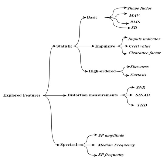
Figure 4.
Representation of features. Totally 15 features (shown in italic) were ex tracted. These features fall into three main categories of statistic, distortion and spectral features.
Statistical Features
Considering Figure 4, statistical features are classified into three fundamental categories of basic features, impulsive metrics, and high-ordered statistics. The specifications of statistical features are described in Table 3. The first category covers the features such as root mean square (RMS), standard deviation (SD), mean absolute value (MAV) and shape factor (SF). The features which fall into the impulse category are associated with the detected peaks in the signal. Impulse components play significant roles in diagnosing aging trend of a signal [26]. Finally, the high-ordered category denotes the features which provide the third or higher power of a sample. Kurtosis and skewness are examples of high-ordered features.
Table 3.
Description of statistical features. In the following equations, presents the total data points in signal , defines the -th value in the signal .
Distortion Metrics
Signal distortion such as noise increment or a variation in a harmonic relative to the fundamental may imply degradation in the signal. There are three popular specifications to measure signal distortion namely signal to noise ratio (SNR), total harmonic distortion (THD), and signal to noise and distortion ratio (SINAD). Mathematical expressions of these measurements are as follow [27]:
According to the aforementioned equations, SNR is specified as the ratio of the amplitude of a signal to noise of the signal and SINAD is defined as the ratio of the signal power level including signal, noise, distortion components over noise plus distortion power. THD measures the distortion existing in the signal and is defined as the total ratio of RMS value of all the harmonic components divided by RMS value of a fundamental signal.
Spectral Features
Spectral features are extracted from the frequency-domain representation of a signal. Therefore, a time-domain signal should be converted to the frequency-domain using power spectrum (PS) or order spectrum methods. In this work, the PS method is selected to present the signal in the frequency-domain. The PS is computed using FFT-based algorithms such as Welch’s or periodogram techniques. According to reference [28], the Welch’s method includes the following steps; in the first step, the time-domain signal is broken into overlapping sections each of length L, in order to variance reduction. Each data section is characterized as:
The next step is applying a window function to each section and for each windowed section computing the periodogram according to Equation (6):
where represent the windowed section.
Lastly, the average value of all sections is applied for calculation of the power spectrum as Equation (7):
There are different window functions that can be used in Welch’s method such as, rectangular window and Hann window which the former is selected in this study.
When the power spectrum of the signal is available, the spectral features can be extracted. Spectrum peak amplitude, spectrum peak frequency, and median normalized frequency of the power spectrum are considered as spectral features which may include essential characteristics about battery degradations.
2.3.2. Prognostic Feature Ranking
Selecting the convenient subset of features out of all extracted features has a tremendous impact on reliable and accurate estimation of SoH. Therefore, feature ranking is applied to identify descriptive features that effectively can track battery degradation. According to [29] there are three common metrics that are broadly applicable for prognostic feature ranking. Monotonicity based on Spearman’s rank correlation coefficient, prognosability and trendability are the suitable criteria to define the prognostic features. These metrics called prognostic metrics.
Monotonicity is a metric for identifying a monotonic trend in a feature. In this research, the monotonicity is formulated based on Spearman’s rank correlation coefficient which is a nonparametric method to evaluate the extent to which a relationship is monotonic, and it is defined as Equation (8) [30]:
where n indicates the number of data points and is the difference in the ranks of sample of observation vector.
Considering Equation (9), monotonicity is defined as follow:
where M is the number of monitored signal, is the vector lifetime points corresponding to the vector of extracted features . A feature has a high degree of monotonicity if its value increases or decreases noticeably through battery degradation trajectory.
Prognosability quantifies the variability of a feature as battery reaches EOL. A feature with a high degree of prognosability presents less variation at EOL. Equation (10) defines the prognosability [31].
where is the value of a feature and represents the total number of measurements of the feature.
Trendability is defined as the similarity among trajectories of a feature from BOL to EOL. As the battery degrades a descriptive feature expresses higher trendability. The following equation demonstrates the trendability metric [29].
As the battery progressively evolves toward EOL, a convenient descriptive feature presents higher values of prognostic metrics. The values of all three prognostic metrics range from 0 to 1. The closer value to 1, a feature is more suitable to be considered as a prognostic feature.
The final score of a feature is calculated based on the sum of these three metrics.
2.4. Ensemble Gradient Boosted Tree
Gradient boosted tree is a sort of ensemble learning method which makes a prediction based on the combination of multiple regression trees [24]. In this method, training of each base-learner is dependent on the base-learner that trained previously, and the final score is calculated by adding prediction of all the trees. The objective of this method is to build a series of trees where each successive tree maximizes the negative gradient of the loss function of the entire ensemble. The negative gradient of the loss function called the pseudo-residuals. Considering the following assumptions, the output of the ensemble gradient boosted tree (EGBT)algorithm is defined according to Table 4 [32]:
Table 4.
Algorithm of the gradient boosted tree (GBT).
- is the training set;
- is the number of leaves;
- are the disjoint regions constitute from input data;
- is the output of region ;
- is a decision tree and its output is calculated as: ;
- is a function that maps to in a way that reduces the loss function over the joint distribution of all ensembles;
- The pseudo-residual is determined as:
There are three main hyperparameters that should be specified initially: (1) the number of trees (iterations), (2) the number of leaves of decision tree, and (3) the learning rate of algorithm (α) which is range between 0 to 1 [23]. Optimum tuning of hyperparameters is a critical step in developing EGBT model which significantly influences prediction accuracy. Early stopping is one of the parameter tuning stages. It determines the minimum number of iterations which is adequate to develop an optimized EGBT. The process of early stopping works by tracking prediction performance on the validation dataset and stopping the training process once the model’s performance doesn’t progress after specific number of iterations. The learning rate is another important parameter to enhance model’s performance. The impact of each weak learner on the final prediction is defined by learning rate. Lower values of learning rate improve model generalization to unseen data. However, the model becomes more complex. Cross-validation RMSE is selected to find an efficient set of hyperparameters using MATLAB functions. The following steps are considered to find the optimal hyperparameters:
- Cross-validate a set of ensembles. Exponentially increase the tree-complexity level for subsequent ensembles from decision stump (one split) to at most n - 1 splits. n is the sample size. In addition, vary the learning rate for each ensemble between 0.05 to 0.2.
- Vary the maximum number of leaves using the values in the sequence {,,…, }. m is such that 2 m is no greater than n − 1.
- For each variant, adjust the learning rate using each value in the set {0.05, 0.1, 0.15, 0.2}.
- Estimate the RMSE for each ensemble.
- Identify the number of trees (N), maximum leaves number of (L), and learning rate (R) that yields the lowest RMSE overall.
K-fold cross-validation was used to understand the efficiency of EGBT model on untrained data. In this technique, the training input is split approximately into K equal parts. In each iteration, K-1 parts are considered as training input and a single part is used for model validation. The entire process is repeated for K fold and all parts are specifically used on time for model validation.
There are various common metrics for assessing the accuracy of estimation. These metrics are listed in Table 5.
Table 5.
List of metrics used for evaluating model performance. N defines observations’ number, and demonstrate the predicted output and the actual target respectively.
3. Results and Discussion
3.1. Experimental Results
In this section, the experimental results will be discussed in detail. First, the aging process of battery cells and various stress factors effecting on battery aging trajectory will be discussed. Second, extracted features will be analyzed according to metrics that are introduced in Section 2.3.2 in order to determine diagnostic features. The performance of EGBT model is evaluated based on performance evaluation criteria which are listed in Table 6. Finally, a comparison between EGBT and decision tree is provided in the discussion section.
Table 6.
Assessing the impact of diagnostic features on prediction performance. The first model uses all extracted features, Model 2 and Model 3 are use the features with total score higher than 1 and 1.5 respectively as training input.
As mentioned before, three cells were cycled under different testing conditions according to Table 2. The aging behavior of cells is illustrated in Figure 5. As the figure shows, each cell presents a distinct aging trend. As can be seen, Cell One reaches EOL after nearly one thousand three hundred cycles while Cell Two with a lower rate of DOD operates much longer than Cell One. On the other hand, despite the similarity of operating conditions of Cell One and Cell Three, SoH of Cell Three approximately reaches 97% after about 1500 cycles due to cycling at low temperatures. Another point is that Cell Three indicates capacity increment during the first 300 cycles. The possible reason for capacity increment is reported in the literature [33]. They suggest that cracking of the positive electrode material grains leads to increase electrode active surface area, and this probably results in capacity increment. The aging results demonstrate that stress factors such as temperature and DOD can significantly affect battery degradation.
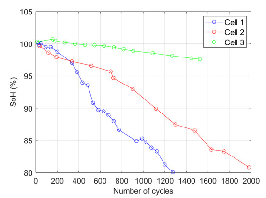
Figure 5.
Battery aging under three different conditions. Comparing the degradation trend of Cell One and Cell Three demonstrates elevated temperature accelerates battery aging. Moreover, the lower rate of depth of discharge (DoD), the capacity fade is less.
Fifteen candidate features are extracted from voltage data. The overview of features is depicted in Figure 4. MATLAB’s parallel computing toolbox was used to accelerate the process of feature extraction. This tool allows for simultaneous feature extraction. The features are then scored based on the metrics which were introduced in Section 2.3.2. The features with a higher value of prognostic metrics are suitable to be selected as diagnostic features. Diagnostic features finally construct the training input for EGBT. Figure 6 illustrates extracted features ranked based on the prognostic metrics.
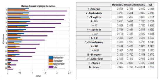
Figure 6.
Order of extracted features. The left-side figure illustrates the order features and the right-side table presents the name of features and their corresponding values. Features are ranked in descending order based on their total score. The total score of a feature is calculated based on the sum of monotonicity, trendability and prognosability.
Three EGBT models were trained to determine what is the promising threshold of prognostic metrics which results in better SoH estimation. The first model was fed with the entire extracted features, while for the second and third models the features with total score higher than 1 and 1.5 are selected as training input for former and latter. The models are compared with regard to precision of estimation and computational cost and results are summarized in Table 6. The computational cost consists of the required time for feature extraction and EGBT training.
It is observed that using the entire set of extracted features as training input, imposes computational burden. What is more, the model accuracy improves as the size of training input reduces. Therefore, Model 2 and Model 3 surpass Model 1. It is also noticeable that the difference between estimation accuracy of Model 2 and Model 3 is marginal, Model 3 however, is computationally less expensive than Model 1. Therefore, Model 3 is predominantly more efficient in online applications due to lower computational complexity. As result, the proposed model achieves the best result with the input data which their prognostics metrics are higher than 1.5 in terms of accuracy and computational costs. Conversely, the features with lower prognostic metrics’ value than 1 are not satisfactory for SoH estimation.
After selecting the input data, initialization of EGBT model will be the next step. As mentioned in Section 2.4, optimum hyperparameters minimize the cross-validation error of predictive model. Thus, selecting optimize hyperparameters has a significant impact on improving prediction accuracy. Three hyperparameters should be set: (1) the number of trees (N) (iterations) (2) the number of leaves (L) of decision tree, and (3) the learning rate of algorithm (R). Herein, to identify optimize hyperparameters four different values of 0.05, 0.1, 1.5, and 2 were chosen as learning rates, the early stopping point corresponds to each learning rate was determined. The figure shows how the cross-validated RMSE behaves as the number of trees in the ensemble increases. The curves are plotted with respect to learning rate on the same plot, and separate subplots are considered for three different values of L. As Figure 7 illustrates, for all learning rates the growing trees considerably improve prediction accuracy. However, one can observe from approximately 100 trees onwards, neither changing learning rates nor increasing the number of trees doesn’t significantly effect on reducing cross-validation error. Yet, smaller learning rate imposes more computational burden. Therefore, the EGBT model is configured with the learning rate value of 0.2 and 100 trees. It was also observed that the best value of decision tree’s leave is eight.
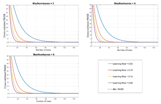
Figure 7.
Impact of hyperparameters on improving prediction error. Although the difference between RMSE in N = 30 and N = 100 is marginal (RMSE30 = 0.319412, RMSE100 = 0.290187), and it is not clear in figure, the best prediction accuracy N = 100, L = 8 and R =.02 was selected by MATLAB function.
Finally, the obtained data from Cell Two are used for training the EGBT model. Cell One and Cell Three are used for validating the accuracy of the developed model. Estimation results, as well as residuals error, for Cell One and Cell Three are depicted in Figure 8.
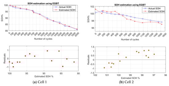
Figure 8.
State of health(SoH) estimation results of (a) Cell One and (b) Cell Three based on ensemble gradient boosted tree (EGBT) model.
The residuals plot depicts the difference between the estimated SoH and actual SoH. As can be observed, the cells which are aged under different conditions can be closely estimated using the developed EGBT model and the residuals scattered roughly around 0. This implies the precision of the predictive model. The performance statistics of tested cells are presented in Table 7. As it is observed all performance evaluation criteria are less than 1%. This also suggests that trained EGBT provides a convenient estimation on untrained data.
Table 7.
Presentation of SoH estimation errors based on performance evaluation criteria.
3.2. Discussion
This section provides comparison between ensemble learning and single decision tree. A decision tree is a prediction model that provides accurate estimation in the training phase, however, it doesn’t well generalize on untrained data. Therefore, combining multiple decision trees can enhance the performance of model. Table 8 shows comparison results between single regression tree and EGBT in training and validation phase. It is notable that Cell Two was used for training and Cell One was used for validation step. As results indicate, both regression tree and EGBT provides convenient estimation in training phase. However, regression tree is surpassed by EGBT model in the validation phase. This confirms that EGBT is capable of estimating SoH of batteries which have distinct aging patterns.
Table 8.
Comparison between the decision tree and EGBT in the training and validation phase.
4. Conclusions and Outlooks
This work proposes a machine learning method to estimate online SoH estimation under dynamic driving conditions. Three NMC cells tested under different conditions using worldwide light-duty driving test cycle profile. Characteristic features were extracted from voltage data and they were scored based on three prognostic metrics called monotonicity, trendability, and prognosability. It was shown that the features which their prognostics metrics are higher than 1.5 are more suitable for SoH estimation in terms of accuracy and computational costs. Conversely, the features with lower prognostic metrics’ value than 1 are not satisfactory for SoH estimation. Finally, an ensemble gradient boosted tree (EGBT) is proposed to estimate the correlation between diagnostic features and battery SoH. To enhance the prediction accuracy and to avoid overfitting of EGBT, the optimum hyperparameters are selected. Moreover, the performance of the proposed method is validated using two different battery cells. The results confirm the convenient performance of the proposed model in estimating battery SoH that operates under various stress factors. Furthermore, it is shown that ensemble learning works better compare to single regression tree in the validation phase. Considering the low computational cost, superb performance in SoH estimation in dynamic driving conditions and robustness of the model, the proposed model is eligible for implementing in battery management systems. The advantage of presented method is its independency to operation variables such as temperature, charging and discharging C-rate, DoD, and etc. Nevertheless, it should be tested on different types of batteries and in various operating conditions to understand the applicability of proposed method. To reach this objective, a large historical dataset of different types of batteries which operate under dynamic conditions should be available. Digital twin technology is a feasible solution to obtain the necessary data to develop a high-precision SoH estimation model. Therefore, the future steps in our research include validating our model using the comprehensive dataset obtaining from digital twin.
Author Contributions
S.K.: Conceived of the presented idea, gathered and processed data, developed the theory and performed the computations, wrote the original draft of manuscript. Y.F.: Were involved in planning and supervised the work, helped in experiments, data analyzing, helped in interpreting the results and worked on the manuscript. M.B.: Were involved in planning and supervised the work, worked on the manuscript. J.V.M.: Contributed to the final version of the manuscript and supervised the work. P.V.D.B.: Contributed to the final version of the manuscript and supervised the work. All authors have read and agreed to the published version of the manuscript.
Funding
This research was funded by OBELICS project grant number 769506 and also supported by Flanders Make.
Acknowledgments
The authors would like to thank the European Commission, Innovation and Networks Executive Agency, which enabled this publication via the Horizon 2020 initiative with the project Optimization of scalable real time models and functional testing for E-drive Concepts (OBELICS) (Grant Agreement Number 769506). We also would like to thank Flanders Make for supporting the battery team in Vrije Universiteit Brussel.
Conflicts of Interest
The authors declare no conflict of interest.
References
- Ali, M.U.; Zafar, A.; Nengroo, S.H.; Hussain, S.; Alvi, M.J.; Kim, H.-J. Towards a Smarter Battery Management System for Electric Vehicle Applications: A Critical Review of Lithium-Ion Battery State of Charge Estimation. Energies 2019, 12, 446. [Google Scholar] [CrossRef]
- Gandoman, F.H.; Jaguemont, J.; Goutam, S.; Gopalakrishnan, R.; Firouz, Y.; Kalogiannis, T.; Omar, N.; Mierlo, J.V. Concept of reliability and safety assessment of lithium-ion batteries in electric vehicles: Basics, progress, and challenges. Appl. Energy 2019, 251, 113343. [Google Scholar] [CrossRef]
- Berecibar, M.; Gandiaga, I.; Villarreal, I.; Omar, N.; Van Mierlo, J.; Van Den Bossche, P. Critical review of state of health estimation methods of Li-ion batteries for real applications. Renew. Sustain. Energy Rev. 2015, 56, 572–587. [Google Scholar] [CrossRef]
- Liu, D.; Yin, X.; Song, Y.; Liu, W.; Peng, Y. An On-Line State of Health Estimation of Lithium-Ion Battery Using Unscented Particle Filter. IEEE Access 2018, 6, 40990–41001. [Google Scholar] [CrossRef]
- Yu, Z.; Huai, R.; Xiao, L. State-of-Charge Estimation for Lithium-Ion Batteries Using a Kalman Filter Based on Local Linearization. Energies 2015, 8, 7854–7873. [Google Scholar] [CrossRef]
- How, D.N.T.; Hannan, M.A.; Hossain Lipu, M.S.; Ker, P.J. State of Charge Estimation for Lithium-Ion Batteries Using Model-Based and Data-Driven Methods: A Review. IEEE Access 2019, 7, 136116–136136. [Google Scholar] [CrossRef]
- Xiong, R.; Li, L.; Tian, J. Towards a smarter battery management system: A critical review on battery state of health monitoring methods. J. Power Sources 2018, 405, 18–29. [Google Scholar] [CrossRef]
- Li, Y.; Liu, K.; Foley, A.M.; Zülke, A.; Berecibar, M.; Nanini-Maury, E.; Nanini-Maury, E.; van Mierlo, J.; Hoster, H.E. Data-driven health estimation and lifetime prediction of lithium-ion batteries: A review. Renew. Sustain. Energy Rev. 2019, 113, 109254. [Google Scholar] [CrossRef]
- Meng, H.; Li, Y.-F. A review on prognostics and health management (PHM) methods of lithium-ion batteries. Renew. Sustain. Energy Rev. 2019, 116, 109405. [Google Scholar] [CrossRef]
- Pan, H.; Lü, Z.; Wang, H.; Wei, H.; Chen, L. Novel battery state-of-health online estimation method using multiple health indicators and an extreme learning machine. Energy 2018, 160, 466–477. [Google Scholar] [CrossRef]
- Guo, P.; Cheng, Z.; Yang, L. A data-driven remaining capacity estimation approach for lithium-ion batteries based on charging health feature extraction. J. Power Sources 2019, 412, 442–450. [Google Scholar] [CrossRef]
- Liu, J.; Chen, Z. Remaining Useful Life Prediction of Lithium-Ion Batteries Based on Health Indicator and Gaussian Process Regression Model. IEEE Access 2019, 7, 39474–39484. [Google Scholar] [CrossRef]
- Deng, Y.; Ying, H.E.J.; Zhu, H.; Wei, K.; Chen, J.; Zhang, F.; Liao, G. Feature parameter extraction and intelligent estimation of the State-of-Health of lithium-ion batteries. Energy 2019, 176, 91–102. [Google Scholar] [CrossRef]
- Li, Y.; Abdel-Monem, M.; Gopalakrishnan, R.; Berecibar, M.; Nanini-Maury, E.; Omar, N.; den Bossche, P.; Mierlo, J. A quick on-line state of health estimation method for Li-ion battery with incremental capacity curves processed by Gaussian filter. J. Power Sources 2018, 373, 40–53. [Google Scholar] [CrossRef]
- Weng, C.; Cui, Y.; Sun, J.; Peng, H. On-board state of health monitoring of lithium-ion batteries using incremental capacity analysis with support vector regression. J. Power Sources 2013, 235, 36–44. [Google Scholar] [CrossRef]
- de Hoog, J.; Timmermans, J.M.; Ioan-Stroe, D.; Swierczynski, M.; Jaguemont, J.; Goutam, S.; Omar, N.; van Mierlo, J.; Van den Bossche, P. Combined cycling and calendar capacity fade modeling of a Nickel-Manganese-Cobalt Oxide Cell with real-life profile validation. Appl. Energy 2017, 200, 47–61. [Google Scholar] [CrossRef]
- Yang, D.; Wang, Y.; Pan, R.; Chen, R.; Chen, Z. A Neural Network Based State-of-Health Estimation of Lithium-ion Battery in Electric Vehicles. Energy Procedia 2017, 105, 2059–2064. [Google Scholar] [CrossRef]
- Khaleghi, S.; Firouz, Y.; Van Mierlo, J.; Van den Bossche, P. Developing a real-time data-driven battery health diagnosis method, using time and frequency domain condition indicators. Appl. Energy 2019, 255, 113813. [Google Scholar] [CrossRef]
- Yang, S.; Wu, J.; Du, Y.; He, Y.; Chen, X. Ensemble Learning for Short-Term Traffic Prediction Based on Gradient Boosting Machine. J. Sens. 2017. [Google Scholar] [CrossRef]
- Singh, S.K.; Kumar, S.; Dwivedi, J.P. A novel soft computing method for engine RUL prediction. Multimed. Tools Appl. 2019, 78, 4065–4087. [Google Scholar] [CrossRef]
- Nenadic, N.G.; Bussey, H.E.; Ardis, P.A.; Thurston, M.G. Estimation of State-of-Charge and Capacity of Used Lithium-Ion Cells. Int. J. Progn. Health Manag. 2014, 5, 12. [Google Scholar]
- Dong, X.; Yu, Z.; Cao, W.; Shi, Y.; Ma, Q. A survey on ensemble learning. Front. Comput. Sci. 2020, 14, 241–258. [Google Scholar] [CrossRef]
- Sagi, O.; Rokach, L. Ensemble learning: A survey. Wiley Interdiscip. Rev. Data Min. Knowl. Discov. 2018, 8. [Google Scholar] [CrossRef]
- Zhang, C.; Ma, Y. Ensemble Machine Learning; Springer: Berlin/Heidelberg, Germany, 1996. [Google Scholar] [CrossRef]
- Chen, X.; Shen, W.; Vo, T.T.; Cao, Z.; Kapoor, A. An overview of lithium-ion batteries for electric vehicles. Int. Power Energy Conf. 2012, 2012, 230–235. [Google Scholar] [CrossRef]
- Deng, S.; Jing, B.; Sheng, S.; Huang, Y.; Zhou, H. Impulse feature extraction method for machinery fault detection using fusion sparse coding and online dictionary learning. Chin. J. Aeronaut. 2015, 28, 488–498. [Google Scholar] [CrossRef]
- Kester, W. MT-003 TUTORIAL Understand SINAD, ENOB, SNR, THD, THD + N, and SFDR so You Don’t Get Lost in the Noise Floor; Analog Devices: Norwood, MA, USA, 2009. [Google Scholar]
- Kunjir, R.; Bhanuse, V.; Kulkarni, J.; Patankar, S. Determination of Deformation of Steel Plate Using Welch’s Periodogram Estimate. In Proceedings of the 2018 Second International Conference on Intelligent Computing and Control Systems (ICICCS), Madurai, India, 14–15 June 2018; pp. 1169–1174. [Google Scholar] [CrossRef]
- Baraldi, P.; Bonfanti, G.; Zio, E. Differential evolution-based multi-objective optimization for the definition of a health indicator for fault diagnostics and prognostics. Mech. Syst. Signal Process. 2018, 102, 382–400. [Google Scholar] [CrossRef]
- Yang, J.; Wang, Y.; Pei, S.; Hu, Q. Monotonicity Induced Parameter Learning for Bayesian Networks with Limited Data. In Proceedings of the International Joint Conference on Neural Networks (IJCNN), Rio de Janeiro, Brazil, 8–13 July 2018; Institute of Electrical and Electronics Engineers Inc.: Piscataway, NJ, USA, 2018. [Google Scholar] [CrossRef]
- Coble, J.; Hines, J.W. Identifying Optimal Prognostic Parameters from Data: A Genetic Algorithms Approach. In Proceedings of the Annual Conference of the Prognostics and Health Management Society 2009, San Diego, CA, USA, 27 September–1 October 2009. [Google Scholar]
- Hastie, T.; Tibshirani, R.; Friedman, J. The Elements of Statistical Learning: Data Mining, Inference, and Prediction; Springer-Verlag: New York, NY, USA, 2009. [Google Scholar]
- Jalkanen, K.; Karppinen, J.; Skogström, L.; Laurila, T.; Nisula, M.; Vuorilehto, K. Cycle aging of commercial NMC/graphite pouch cells at different temperatures. Appl. Energy 2015, 154, 160–172. [Google Scholar] [CrossRef]
© 2020 by the authors. Licensee MDPI, Basel, Switzerland. This article is an open access article distributed under the terms and conditions of the Creative Commons Attribution (CC BY) license (http://creativecommons.org/licenses/by/4.0/).