The Cost-Optimal Analysis of a Multistory Building in the Mediterranean Area: Financial and Macroeconomic Projections

Abstract

Cost-optimal analysis was pointed out in the 2010/31 European Directive as a tool to evaluate the achievable building energy performance levels as a function of the corresponding costs. These analyses can be carried out by a financial projection for private investors and a macroeconomic approach to establish the minimal energy performance levels. Consequently, the financial projection provides different results that could stimulate private investors toward other cost-optimal solutions that do not match the minimal energy performance levels. For this purpose, both the projections were analyzed in the BEopt environment, developed by NREL, on a multistory building located in two contrasting climatic zones of the Mediterranean area, one cold and the other warm, highlighting the differences. The cost-optimal solutions were identified by a parametric study involving measures that affect thermal losses and solar gains, whereas the air-conditioning plant was left unchanged in order to include a fraction of renewable energy in the coverage of the building demands. Results showed that both the projections produced the same cost-optimal solutions, however, the latter matches the building designed to fulfill the minimal energy performance levels only in the cold climate. Conversely, noticeable deviations were detected in the warm location, therefore minimal energy performance levels should be revised, with preference for less insulated opaque surfaces and better performing glazing systems. Moreover, the macroeconomic scenario returns a more limited distance between the minimal energy performance levels and the cost-optimal solutions, therefore, it is far from the real economic frame sustained by private investors.

1. Introduction

Modern economy is based on the energy availability to guarantee development and benefit for society, the improvement of life quality and to satisfy human needs. In the EU, energy demand is strongly affected by the building sector that is responsible for 40% of the global energy consumption for final uses and for 36% of CO₂ emissions, with a residential sector that contributes by itself for 25.4% of the total demand [1,2,3]. Consequently, the spread of residential nZEB (nearly Zero Energy Buildings) [4] constitutes an appropriate strategy aimed at reducing the EU energy dependence and for limiting pollutant emissions. Clearly, suitable legislative plans have been developed in order to improve energy efficiency politics, as well as energy savings interventions and integration of renewable systems in the building sector. However, all these targets have to be attained in regard to a sustainable economic frame, as stated by article five of the 2010/31 European Directive [5,6]. The idea to design new buildings as nZEB with reduced investment costs, in fact, is still too far from an actual application. Other building configurations, instead, appear more attractive due to cheaper initial investments that result in more favorable outcomes despite a slight increase in running (operating) costs. Consequently, the building–plant system with the lowest energy demand represents the cost-optimal solution; conversely the latter can be identified as a favorable balance point between energy consumption, investment and operational costs [7]. The 2010/31 EU directive represents the first attempt for the definition of a comparative methodological framework for the calculation of the optimal energy performance levels as a function of the costs, with reference to new and existing buildings [8]. The procedure cannot be generalized across Europe, therefore Member States have to adapt it to the climatic context, the accessibility to the energy infrastructures and the local market. In order to overcome these drawbacks, appropriate guidelines (Regulation 244) [9] were formulated to support the implementation of the cost-optimal procedure in every country by different steps:

• Definition of a reference building (RB) relative to its functionality and climatic context;
• Identification of the energy efficiency measures (EEM) that apply to the RB at a global level or on the single component or on their combination;
• Evaluation of the energy performance levels before and after the interventions, in accordance with the European technical standards;
• Global cost calculation in accordance with the net present value (NPV) concept and the international standard EN 15459:2008 [10], taking into account initial, operative, maintenance and disposal costs;
• Sensibility analysis on the costs as a function of different energy carriers;
• Identification of the optimal solutions as a function of the cost and the corresponding energy performance levels.

The economic analysis can be carried out in two different ways. The financial projection, in which actual economic indexes are used and all the charges are included in the formation of the costs, is suitable for private investors. Alternatively, the macroeconomic projection, where the costs have to be evaluated by excluding every typology of taxes, but including the CO₂ emissions cost and applying a lower discount rate index than the prior case, can be used to emanate building regulations [11]. Indeed, at a national level, Member States use the results obtained with the macroeconomic projection to define the minimal energy performance requirements in buildings. Nevertheless, they have to verify periodically that the minimal energy performance requirements do not produce a worsened scenario than the energy performances corresponding to the cost-optimal solution. For instance, the latter could be subjected to variations due to the oscillations of the energy carrier costs. If the deviances are greater than 15%, appropriate modifications to the national legislation should be produced.

The general purpose of this paper is to perform the cost-optimal analysis by using the two economic projections, which will quantify the deviances in terms of corresponding costs detected on a reference building. The cost-optimal approach was widely considered in recent literature to identify suitable EEMs for the design of new buildings or for refurbishment planning. However, the majority of these investigations regard dominant heating climates. For instance, in [12] a cost-optimal approach for the identification of suitable insulation materials to adopt in the refurbishment of historical buildings was carried out, but the analysis was limited to heating applications because the RB was located in the Prealps with a prevalent continental climate. A cost-optimal analysis aimed for the attainment of nZEB schools located in Northeast Italy was carried out in [13], considering only the heating requirements due to the particular intended use. A school building was also investigated in [14] to define the optimum insulation thickness and the best glazing system by locating the edifice in a mountain city of South Italy. In [15], specific EEMs were contemplated for a Czech building stock, creating the basis for calculating the cost-effective solution at a national level. Finally, a study concerning the renovation of Swedish multistory buildings is reported in [16] by considering only heating and domestic hot water production, however, no information was provided for the design of new structures. Other investigations can be found for buildings located in warm climates, such as the Mediterranean area, where the role of cooling demands cannot be neglected. The involvement of the cooling requirements makes the cost-optimal analysis and the identification of suitable EEMs difficult, often because solutions employed to reduce heating needs produce cooling demand growth, and vice versa. Cooling requirements were involved in [17], where appropriate EEMs were identified specifically for the refurbishment of the typical Italian social housing stock. Furthermore, in [18] a cost-optimal analysis was developed for reference buildings located in each of the three different climatic zones of Cyprus, limiting the investigation only to the main components of the building envelope, without considering the replacement of the technical plant. In [19], by means of the results provided by the European project RePublic_ZEB, a cost-optimal analysis was carried out to achieve public nZEB located in five different countries, considering requirements for both heating and cooling. The cost-optimal analysis was the approach employed for the design of a new prototype of residential buildings, as shown in [20] where cost-effective nZEBs were achieved for different localities across Europe, highlighting also the role of appliances and lighting on energy consumption. With reference to the European situation, other studies focusing on the role of cooling demands were carried out in [21] but specifically for non-residential buildings located in Serbia. In [22], a cost-optimal analysis was conducted for warm climates in order to carry out a comparison between standard and high-performance, single residential buildings in the design phase. A multistory building, representative of existing Italian building stock, was investigated in [23] by proving the feasibility of nZEB in warm climates, especially in presence of massive structures. However, only the macroeconomic projection was employed, highlighting that it is very difficult to reduce the gap between cost-optimal and lowest energy consumption solutions. Finally, Portuguese buildings were investigated in [24] by considering both heating and cooling, but the cost-optimal analysis was addressed exclusively to the renovation of existing residential edifices. In

Table 1. Synoptic framework of the main documents found in literature, providing authors, economic scenario (F = Financial, M = Macroeconomic), energy services (H = Heating, C = Cooling, DHW = Domestic Hot Water, A = Appliance) and building typology (R = Residential, NR = Nonresidential).

Authors	Economic Scenario	Energy Services	Building Typology
Lucchi et al. [12]	M	H	R (historical)
Mora et al. [13]	F	H	NR (school)
D’Agostino et al. [14]	F/M	H	NR (school)
Karásek et al. [15]	M	H/DHW	R/NR
Bonakdar et al. [16]	F	H/DHW	R (multistory)
Carpino et al. [17]	M	H/C/DHW	R (social housing)
Loukaidou et al [18]	F	H/C	R/NR (nZEB)
Aelenei et al. [19]	Not indicated	H/C/DHW	NR (office)
D’Agostino&Parker [20]	F	H/C/DHW/A	R (two-story)
Stevanović [21]	Not indicated	H/C	NR (office)
Baglivo et al. [22]	F/M	H/C/DHW/A	R (single-story)
Zacà et al. [23]	M	H/C/DHW/A	R (multistory)
Brandão De Vasconcelos [24]	F/M	H/C/DHW	R (existing)

, a list of the literature noted is summarized by highlighting the economic scenario followed, the energy services considered and the building typology investigated.

Clearly, a comparison between the cost-effective solutions provided by financial and macroeconomic projections for a large building located in the Mediterranean area is missing. For this reason, this document describes a parametric study carried out on a multistory building located in contrasting climatic zones to develop an optimized building envelope by means of the cost-optimal approach. Indeed, the main goal of this paper is the comparison between the solutions provided by the two economic scenarios and, eventually, to evaluate if private investors could be attracted by more favorable measures than those imposed by current regulations. Moreover, regarding the more influential features of the building envelope, the same analyses allow verification if the macroeconomic projection produces an optimal solution that matches the constraints imposed by regulations, in order to validate the minimal energy performance levels currently adopted in both the climatic zones. Finally, from the comparison between the two projections, the role of CO₂ emissions on the results obtained can be quantified.

2. Description of the Multistory Residential Building Considered

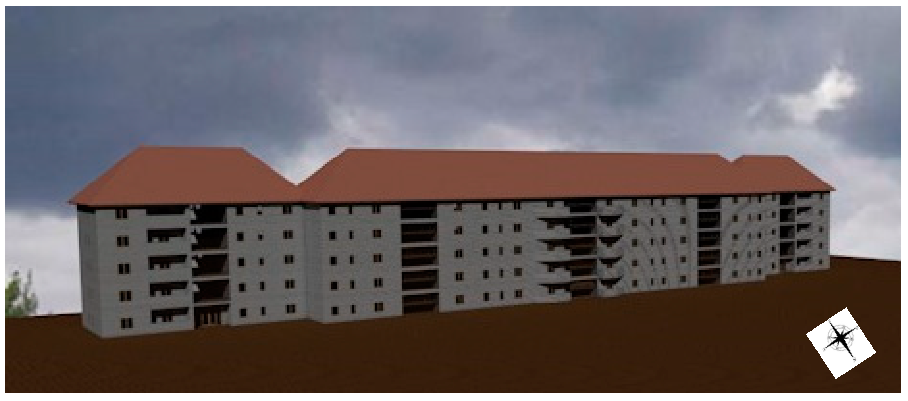
In the cost-optimal analyses, a building benchmark is required and this configuration is represented by the building–plant system that complies with all the measures in terms of minimal energy performance levels, as set by Italian legislation for the climatic zone considered, including a fraction over 50% of primary energy requirements provided by renewable sources [25]. The envelope morphologically consists of a single structure about 60 m long, with the ending modules (each about 20 m long) shifted back 5 m, configuring three well-identified blocks with a depth of about 10 m, see Figure 1. It was developed with five stories above the ground and a floor height of 2.85 m, with a neither habitable nor air conditioned attic. The large structure size was chosen in order to detect a greater impact of the CO₂ emissions for the provision of heating, cooling and domestic hot water.

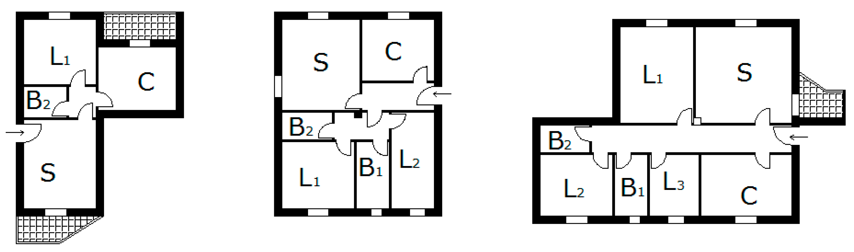
Three different types of apartments were developed, as depicted in Figure 2, where all the rooms, including the corridor, were designed as conditioned indoor environments. The apartments were classified as a function of the net conditioned area as:

• Small, about 60 m²;
• Medium, about 80 m²;
• Large, slightly over 120 m².

In every floor (excluding the attic), two small, two large apartments and six medium flats were distributed around five external stairwells. Globally, the building included a total of 50 apartments for a total conditioned surface of about 4200 m².

For the energy evaluations, the building was located in a warm location (zone B) characterized by 899 winter degree-day (WDD) and 977 summer degree-day (SDD). The second cold location (zone F) was characterized by 3959 WDD and 74 SDD [26] with dominant heating needs. The structure was constructed of framed reinforced concrete. The external walls were developed with an internal plaster 2 cm thick with a thermal conductivity of 1 W/m∙K, a hollow brick of 30 cm with thermal resistance of 0.79 m²∙K/W and a commercial ETICS panel (External Thermal Insulation Coating System) with thermal conductivity of, 0.0595 W/m∙K), whose thickness varied as a function of the climatic zone to provide the thermal transmittance values listed in

Table 2. Thermal transmittance of opaque walls (with correspondent insulation thickness in cm in round brackets) and windows (with normal solar factor of glazing in round brackets) for the building benchmark in climatic zones B and F.

Climatic Zone	Thermal Transmittance (W/m2K), Insulation Thickness (cm) and Normal Solar Factor (-)
	Vertical Wall	Basement Floor	Second-Last Floor	Windows
B	0.43 (8)	0.44 (8)	0.35 (10)	3.00 (0.75)
F	0.24 (15)	0.24 (15)	0.20 (18)	1.10 (0.60)

. Corresponding insulation thickness are indicated in centimeters (Table 2, values in round brackets). For the dynamic performances of opaque walls subjected to the solar radiation, in every building configuration surface mass greater than 250 kg/m³ and periodic thermal transmittance lower than 0.06 W/m²K were attained [25].

Regarding the non-dispersing surfaces, such as the horizontal inter-floor and vertical walls separating different apartments, a thermal transmittance of 0.8 W/m²K was imposed, as well as for the pitched roof. Every room was equipped with a transparent surface whose area was set to one-eighth of the floor surface to exploit daylight adequately. Table 2 also reports window thermal transmittance and the corresponding normal solar factors (round brackets). In accordance with the minimal energy performance levels, a wooden frame mounting two clear glasses 4 mm thick with 12 mm of air-gap was required for the warm location. For zone F, instead, three panes 4 mm thick with the two external glasses subjected to low emission treatment and argon-filled in two 8 mm spaces were necessary [27]. The control of solar gains, especially crucial in the warm location, was modeled by using rolling shutters, controlled as a function of the exposure and time of the year, and by setting the reduction factors listed in

Table 3. Solar gain reduction factors set for the investigated building, as a function of the exposure and for the month, used to manage solar shading devices during simulations (diurnal hours).

	North	East	South	West
Jan	1.00	0.72	0.57	0.79
Feb	1.00	0.74	0.56	0.71
Mar	1.00	0.65	0.57	0.66
Apr	1.00	0.62	0.61	0.67
May	1.00	0.62	0.67	0.66
Jun	1.00	0.60	0.70	0.64
Jul	1.00	0.61	0.67	0.61
Aug	1.00	0.60	0.59	0.62
Sep	1.00	0.61	0.56	0.64
Oct	1.00	0.62	0.54	0.68
Nov	1.00	0.67	0.55	0.84
Dec	1.00	0.73	0.54	0.78

when incident solar radiation exceeded 300 W/m² [28]. In winter, instead, the same devices were considered fully closed during the night to reduce thermal losses. Internal gains of 352, 413 and 450 W for the apartments of 60, 80 and 120 m², respectively, and a natural ventilation with 0.5 air-change per hour, in accordance with Italian standards, were set [29]. Finally, energy requirements for heating and cooling have been determined with indoor set-point temperatures of 20 °C in winter and 26 °C in summer [29].

The air-conditioning plant was modeled as a split system (air–air heat pump) in every room, opportunely sized as a function of the cooling loads for Zone B and for heating in Zone F. No power integration was considered in winter because of the cut-off temperature of −10 °C and the bivalent temperature of −7.7 °C for Zone F. Independent heat pump water heaters (HPWH) were located in every bathroom to produce domestic hot water (DHW), satisfying the requirements calculated by setting a daily volume of hot water equal to 100, 122 and 165 L for the small, medium and large apartments, respectively [30].

Beyond the aerothermal source, the renewable fraction in the building–plant system benefits from a photovoltaic (PV) generator installed on the roof tilted southward and with a peak power of 16.1 kW_p [31]. The renewable electricity was considered totally absorbed by heat pumps (if their operation is required) when energy surplus was not detected. When the electricity demand was greater than the PV production, the remaining part was absorbed from the external grid, conversely in presence of surplus, the renewable electricity was delivered outward.

3. Methodology

The cost-optimal analyses found in literature and previously mentioned were carried out by employing different tools for the energy performance analysis, for the optimization criteria or both [32]. Suitable software, in fact, was necessary to determine energy requirements as a function of a large number of possible combinations of measures, by considering different building envelope configurations, several energy provision systems, as well as the presence of renewable sources, thus requiring a large number of simulations [33]. Successively, an economic analysis with actualized costs had to be carried out in order to analyze the same EEMs also in monetary terms. Both these features can be attained simultaneously by using BEopt v. 2.8 (Building Energy Optimization tool), developed as freeware tool by NREL, the national renewable energy laboratory of the U.S. Department of energy, that can be considered as an Energy Plus front-end, aimed at the cost-optimal analysis of buildings [34]. The EnergyPlus engine was used for the calculation of the primary energy requirements for heating, cooling, domestic hot water and also lighting and appliances if needed, by separating the fossil and the renewable contributions and quantifying the CO₂ emissions required for the macroeconomic projection. In presence of renewable sources, the annual net primary energy, defined as the difference between the actual energy employed for the provision of the energy services and that exported outwards, was also evaluated. Since software and database were developed mainly for the North America context, appropriate adjustments were necessary. However, BEopt is highly flexible, allowing for the analysis of several building typologies in specific climatic contexts by introducing personalized components, upgrading the cost modules and including the economic indexes, as well as the use of an apposite weather database. In this regard, BEopt was used in [35] to investigate an optimal nZEB design characterized by the lowest costs in fourteen different locations across Europe, with particular reference to a single-story structure. Moreover, BEopt was used in [36] to investigate the cost-effectiveness of residential building stock retrofits in Italy and Denmark. BEopt was also used in [37] for building optimization in different Japanese cities.

The investigated building was simulated with different insulation thicknesses in the opaque dispersing walls and by equipping the envelope with two different glazing systems. This was done to investigate other configurations and to compare energy performances with the RB. These parameters affect thermal losses and solar gains and an optimal compromise had to be found to minimize the annual energy demand. Conversely, the air-conditioning plant for the provision of heating and cooling was maintained unvaried by always considering the use of electric air–air heat pumps. The choice to analyze these devices as a generation system exclusively was due to different reasons. Firstly, the same air conditioning system can be used for the provision of heating and cooling, resulting as less invasive from the installation point of view and consequently economically more attractive. Secondly, heat pumps assure the coverage of a noticeable fraction of the building requirements by means of the aerothermal renewable source [31]. Finally, these devices are able also to exploit the renewable electricity, rationalizing the electricity produced by the PV generator installed to meet the Italian regulation in terms of integrating renewable systems in buildings [31]. For the same reasons, the HPWHs equipped with electrical boosters were considered as an unchangeable system for the production of DHW. Despite that it affects the results noticeably [38], the influence of occupant behavior was not considered in the energy analysis because the main goal of this paper was the optimization of the building–plant system during the design process

For the financial and the macroeconomic projections, the cost-optimal analysis results were displayed in terms of annualized energy-related costs against the fossil contribution in the formation of the annual net primary energy absorbed from the grid. The first were defined by considering the electricity expenses sustained in the lifespan, annualized by a capital recovery factor and incremented by the EEM costs (and CO₂ emission cost in macroeconomic evaluations), obtaining more reduced values when compared with the items provided by the life cycle cost (LCC) analysis. For the purpose of this work, the CO₂ emissions were determined as a function of absorbed electric energy from the grid, whose production also requires the employment of fossil primary sources. As a precaution, a conversion factor of 1.95 to transform electricity into fossil primary energy was set constant for the whole building–plant lifespan, because of the high production percentage already obtained by means of renewable systems (especially photovoltaic and hydroelectric) and the massive use of natural gas in fired power plants [25]. Successively, appropriate emission factors related to the current Italian power generation system were employed [39].

Regarding the EEMs considered, the reference building was modified by including two improving and one worsening intervention, the latter to verify also if the cost-optimal solution could be detected in the presence of a pejorative energy scenario. The modified configurations present the same characteristics in terms of shape and orientation, whereas the thermal and optical properties of the envelope were varied. The potential optimization actions attainable by specific EEMs involve the reduction of the transmission losses through the dispersing surfaces and the optimization of solar gains through the glazing systems, the latter crucial for the reduction of the cooling requirements and avoiding the worsening of heating needs. These analyses were aimed at the identification of the optimal insulation thicknesses and the more appropriate windowed system to adopt in the building envelope, for the specific climatic context. In order to limit the simulation times, four different insulation thicknesses were considered for each of three dispersing surfaces, whereas two different typologies of glazing systems were investigated, producing 128 combinations of different measures. In detail,

Table 4. Insulation thicknesses and thermal transmittances of opaque walls (VW, vertical wall; GS, ground slab; SF, second to last floor), thermal transmittances and normal solar factors of the windowed systems in climatic zones B and F.

Opaque Walls					Windowed Systems
CLIMATIC ZONE		Insulation Thickness (cm), Thermal Transmittance (W/m2K)			Thermal Transmittance (W/m2K) Normal Solar Factor (-)
		VW	GS	SF
B	4	0.60	0.62	0.46	3.00 75%
	8	0.43	0.44	0.40
	10	0.38	0.38	0.35	1.10 60%
	12	0.33	0.24	0.31
F	10	0.30	0.31	0.27	3.00 75%
	15	0.24	0.24	0.22
	18	0.21	0.20	0.20	1.10 60%
	20	0.20	0.20	0.19

lists the values of the insulation thicknesses and the corresponding thermal transmittances, the thermal transmittances and the normal solar factors of windows in the simulated building-plant configurations.

For the cost analysis, the approach adopted was based on the evaluation of the annualized energy-related costs, increased by the EEMs cost and determined in accordance with EU Regulation 244/2012 [9,10]. In particular, the economic analysis involved construction, management and maintenance costs of the building–plant system, beyond the operative (or running) costs derived from energy consumption during the lifespan, which the same regulation sets in 30 years for residential buildings. Since running costs are extremely volatile during the mean-long periods, their actualization to the initial years (when the initial investment is sustained) by means of appropriate inflation and discount rates, was required. For financial evaluations, the economic indexes employed in the cost-optimal analysis were set to 4% for the discount rate that represents the maximum interest that investors could obtain by an alternative safe investment. Currently, the latter are represented by a deposit account with restricted funds (generally greater than one year) that have a better yield than thirty-year government bonds. Greater discount rates were not considered because the latter represent the more favorable situation for a private investor, whereas a lower discount rate was contemplated in the macroeconomic projection. Regarding the other economic indexes, 0.3% was set for the general inflation rate [40] and 3.2% for the energy carrier inflation rate (electricity) [41].

Table 5. Economic indexes employed for the economic projections.

Economic Scenario	Discount Rate	General Inflation Rate	Energy Inflation Rate
Financial	4%	0.3%	3.2%
Macroeconomic	2%	0.3%	3.2%

lists the economic indexes employed in both economic scenarios.

For macroeconomic projections, only the discount rate was changed to 2% in order to consider a discount rate lower than that available on the market, as prescribed by regulation. The CO₂ emission cost was determined at annual level as an additional term in the evaluation of the global costs of the building-plant system. Nevertheless, the same regulation set a constant flat rate of 20 €/ton per year (valid until 2025) as stated by the current commission forecast of the carbon prices of the ETS (Emission Trading System) of the European Commission. It is worth mentioning that the CO₂ emission cost is very dissimilar from that found in literature; for instance, an average value of 375 € per ton of emitted CO₂ per year was determined in [42]. However, beyond the environmental costs, this is comprehensive of other items (for instance the social costs connected with human health effects).

For each package of measures, BEopt determined internally the corresponding NPV (Net Present Value) starting from the corresponding cost, also including installation costs. The NPV is usually employed in capital budgeting and investment planning to analyze the profitability of a projected investment. It is defined as the difference between the present value of cash inflows and outflows over a period of time. The construction costs that do not produce deviances in the comparison of the different building configurations (for instance structural frame, foundations, internal partitions or wall finish) were not considered. The different constructive solutions that minimize the global costs as a function of the different levels of energy savings were identified by adopting a sequential search optimization technique on discrete packages of measures to consider realistic design options. Because EU regulation establishes that measured costs have to be determined as a function of market investigations, a local regional data base [43], coherent with the locations and the construction times, was adopted. These lists include the installation costs, the transportation and the costs concerning the rental of machinery and equipment, provided per unit of surface or per component. The regional price lists guarantee cost uniformity across the involved territory, as well as adequacy to the market value, defining average costs for every component and material. In

Table 6. Initial investment costs required for the reference building (RB) in climatic zones B and F, classified as a function of the main expense components.

Total Initial Investment
Components	Financial Projection Zone F		Macroeconomic Projection
	Zone B	Zone F	Zone B	Zone F
	Costs (€)	Costs (€)	Costs (€)	Costs (€)
External Walls	849,937	1,148,000	798,197	1,078,116
Top Floor + Roof	79,666	103,389	73,300	95,128
Foundations + Basement	25,157	35,717	23,303	33,084
Internal Partition + Floor decks	300,327	300,327	283,074	283,074
Windows & Doors	127,384	146,883	103,667	119,536
Rolling shutters	25,154	25,154	20,770	20,770
Air Conditioning	257,265	266,252	205,860	213,051
Domestic Hot Water	115,832	115,832	91,230	91,230
PV Generator	25,766	25,766	21,262	21,262
INITIAL INVESTMENT	1,806,488	2,167,320	1,620,663	1,955,250

, the investment costs, as well as the main specific costs concerning the envelope and technical plants for the building benchmark located in the two climatic zones, are listed. It is worth mentioning that in the financial projection, a VAT of 4% was applied to the EEM components that were involved. Clearly, in zone F, the greater insulation thicknesses and the windows equipped with triple pane were major initial investments when compared to the RB in zone B (about 17%), as well as the air-conditioning plant due to the greater required heating power and the correspondingly larger size heat pumps. Taxes, excises and other charges were not considered in the macroeconomic projections. At annual level, the sustained costs were considered to involve building–plant management (running costs) and ordinary maintenance. In the formation of the running costs, by considering that the adopted energy carrier was represented exclusively by electricity, an average energy cost was evaluated at national level by considering the price determined for the quarter January–March 2019 [41]. In this regard, in BEopt, a user-specified electricity price as a function of the time of intended use, was implemented. In particular, three hourly intervals were set and distinguished with F1, F2 and F3 [41]. The corresponding electricity prices are listed in

Table 7. Average electricity price determined for the quarter January–March 2019 concerning the Italian market, as a function of the three intervals defined by the time for intended use.

Italian Electricity Price (€/kWhe)
	F1: from Monday to Friday 8:00–19:00	F2: from Monday to Friday 7:00–8:00 and 19:00–23:00 Saturday 7:00–23:00	F3: from Monday to Saturday 23:00–7:00 Sunday and Holidays
Financial	0.19615	0.18613	0.18613
Macroeconomic	0.15384	0.14482	0.14482

including, in the financial projection, excises of 0.0227 €/kWh_e and VAT of 10%. The same costs were reported without charges for the implementation of the macroeconomic projection. The PV electricity surplus delivered to the grid, due to the very limited average sales price (about 0.04 €/kW) [44] and the different production achievable among the climatic zones considered, was neglected and not included as positive cash flow to reduce the annual running costs. Finally, periodic costs were considered for the substitution of components due to obsolescence and wear, assuming the replacement times listed in

Table 8. Replacement times assumed for the main building–plant system components in a lifespan of 30 years.

Considered Duration (years)
Typology	Components/Systems	Years
Building envelope	Concrete masonry unit	Not replaced
	External insulation system	Not replaced
	External plaster	30
	Windowed system	30
	Roof slab	Not replaced
	Roof covering	30
	Foundations	Not replaced
HVAC	Heat pumps	15
HPWH	Heat pump water heater	12
Renewable system	PV generator	25

[9]. Building-envelope components were not replaced during the lifespan considered, whereas HVAC systems, HPWH and PV panels were changed at least one time during the economic analysis. These features allow for the depiction of the annualized energy-related costs corresponding to the different packages as a function of the net primary energy from fossil fuels. The annual CO₂ emissions costs for every building configuration were quantified only in the macroeconomic projection.

4. Results and Discussion

Every package of measures was characterized by a precise value of the annual primary fossil energy demand and the corresponding energy-related annualized costs, opportunely plotted. Thus, the set of the packages considered determined a graph where the frontier points in the lowest part denote the Pareto front, representing the geometrical place that joins the optimal outcomes with a broken line. No points can be detected beyond the Pareto front, with the EEMs close to the y-axis that indicate interventions characterized by lower primary energy demands but higher costs, whereas the points close to the x-axis represents interventions that lead to lower costs but higher primary energy requirements and CO₂ emissions. Usually, the solution with the lowest annualized energy-related cost identifies the cost-optimal solution. In the graphs, only some representative points with remarkable results were highlighted. In particular, in every graph the points listed in

Table 9. Points indicating of the more representative building configurations.

Point	Description
COS	Cost-optimal solution with the lowest annualized energy-related cost
RB	Building benchmark designed as a function of the minimal energy performance levels
EEB	Building configuration with the lowest primary fossil energy demand
PEJ	Pejorative solution than minimal energy performance levels
MEC	Building configuration with the highest energy consumption
MC	Building configuration with the highest cost
OP1	Other building configuration belonging to the Pareto front
OP2	Further building configuration belonging to the Pareto front
OP3	Further building configuration belonging to the Pareto front

were emphasized.

Moreover, the other three combinations of interventions belonging to the Pareto front were considered, because these were representative of other alternative cost-effective solutions, and are indicated as OP1, OP2 and OP3. For every point considered, the deviances with COS (cost-optimal solution with the lowest annualized energy-related cost) were determined both in terms of costs and energy demands. The same procedure was carried out for both scenarios, in order to evaluate the differences between the building configurations considered when two different approaches concerning the economic analyses were carried out. Furthermore, in the macroeconomic projection, COS and RB (building benchmark designed as a function of the minimal energy performance levels) should be very close in order to verify if minimal energy performance levels were formulated as a function of the cost-optimal solution, as stated by the European regulations.

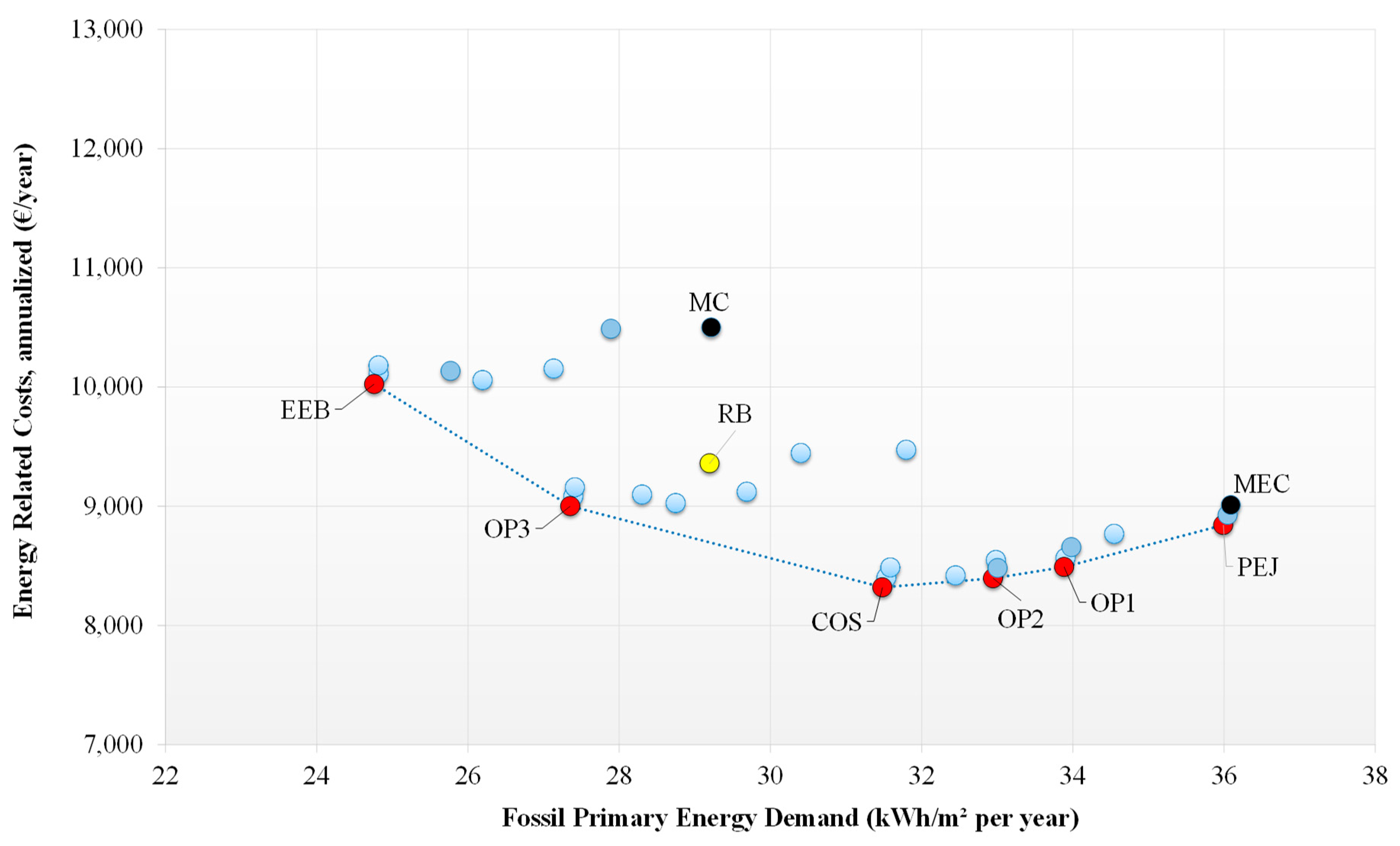
4.1. Cost-Optimal Analysis with Financial Projection

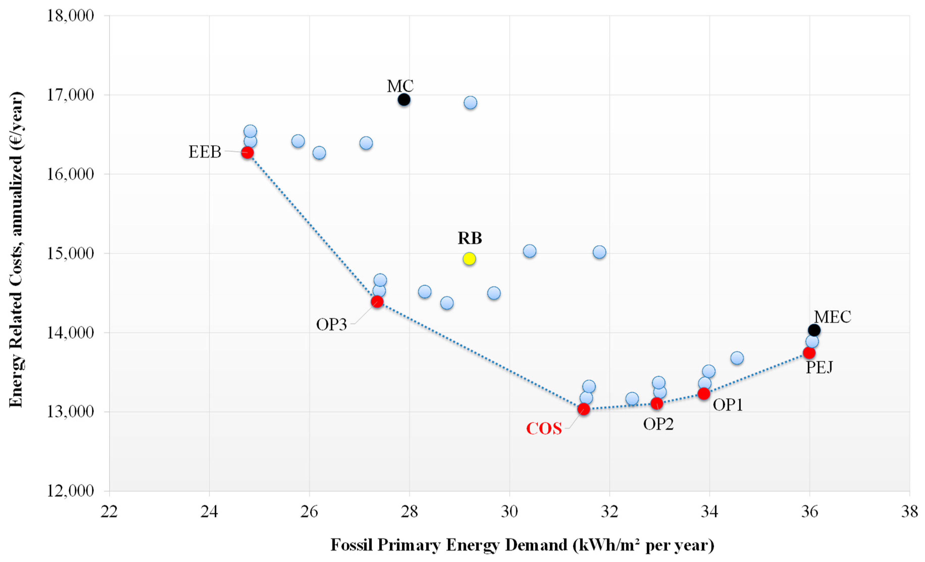
In accordance with the standard EN 15459, the annualized energy-related costs against the fossil primary energy demand provided by BEopt for climatic Zone B are shown in Figure 3. In

Table 10. Detected optimal constructive solutions concerning different energy efficiency measures (EEMs) for climatic zone B (VWT, insulation thickness in vertical wall; GST, insulation thickness in the ground slab; SFT, insulation thickness in the second last floor; GS, glazing system).

EEMs	VWT	GST	SFT	GS
PEJ	4 cm	4 cm	4 cm	Double pane
OP1	4 cm	4 cm	8 cm	Double pane
OP2	4 cm	4 cm	12 cm	Double pane
OP3	8 cm	4 cm	12 cm	Triple pane
RB	8 cm	8 cm	10 cm	Double pane
EEB	12 cm	4 cm	12 cm	Triple pane
MEC	4 cm	12 cm	4 cm	Double pane
MC	12 cm	4 cm	4 cm	Triple pane
COS	4 cm	4 cm	12 cm	Triple pane

, the results corresponding to the constructive solutions for each point considered are specified.

Clearly, for the climatic context considered, the deviances in terms of cost between the COS and the RB point are evident; the latter produces an annualized extra cost of 1900 €, against a primary energy saving of 2.4 kWh/m². It means that, for the considered location and from the financial point of view, investors should prefer a solution energetically less efficient than that suggested by Italian legislation, because the reduction of the costs related to the attainment of the COS measures prevails on a slight annual running cost growth due to the higher electricity consumption. Moreover, the cost-optimal solution is placed on the right side of the graph, meaning that in the warm location the point economically looks more favorable toward greater energy consumption. The EEB solution allowed for reducing the primary energy demand to 24.9 kWh/m², with an energy saving of 17% and 26.5% when compared with RB and COS, respectively. However, the annualized extra cost increase of 3250 € (+25%) and 1300 € (+8.7%) make the result unattractive. The solutions OP1 and OP2 offer similar costs to the COS solution; however, the primary energy demands are slightly higher, therefore these packages of interventions are not recommended. Conversely, OP3 determined an augmented annualized global cost of about 1300 € (+10%); however, the primary energy demand was reduced significantly to 27.3 kWh/m², resulting in OP3 being more favorable than EEB. Finally, the PEJ point produced similar results to the MEC point and both were more expensive than COS. Therefore, the running cost growth due to the limited insulation thicknesses and the cheapest installed window system prevailed on the reduction of investment expenses. The analysis of the values listed in Table 10 suggests that in the warm location, the solution of a scarcely insulated ground slab is always preferred, whereas reduced insulation thicknesses in the dispersing vertical walls are recommended when triple pane systems are installed. Considering the cooling-dominant location, in fact, in summer the first allows for dissipation of thermal power toward the soil, and the second one permits the attainment of the best compromise between the augmentation of thermal losses and the limitation of solar gains. It is worth highlighting that, conversely to the cost-optimal solution, the EEB requires an envelope that is highly insulated, excluding the ground floor and glazing with reduced normal solar gains. The COS point, instead, requires only a large insulation thickness on the second last floor, whereas the thicknesses inside the vertical walls and ground slab are halved compared to those imposed by minimal energy performance levels. This is in agreement with [45], where excessive insulation thicknesses are not recommended for an office building in a warm climate, with thicknesses that have to be further reduced in the presence of high internal gains. In another investigation [11], instead, a reference office building in a warm climate met the nZEB target in conjunction with a favorable economic frame only when the building fabric is characterized by high thermal inertia.

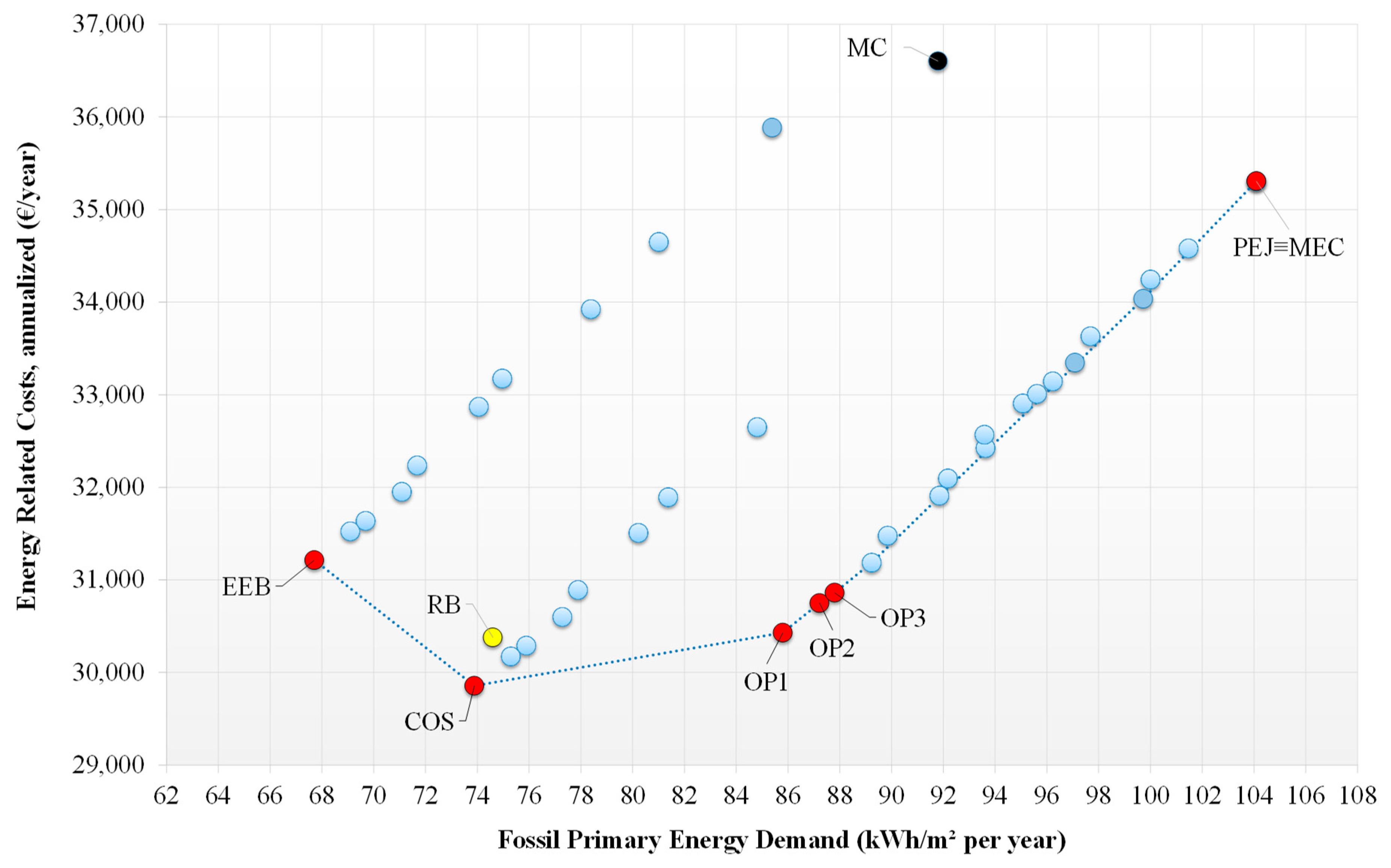
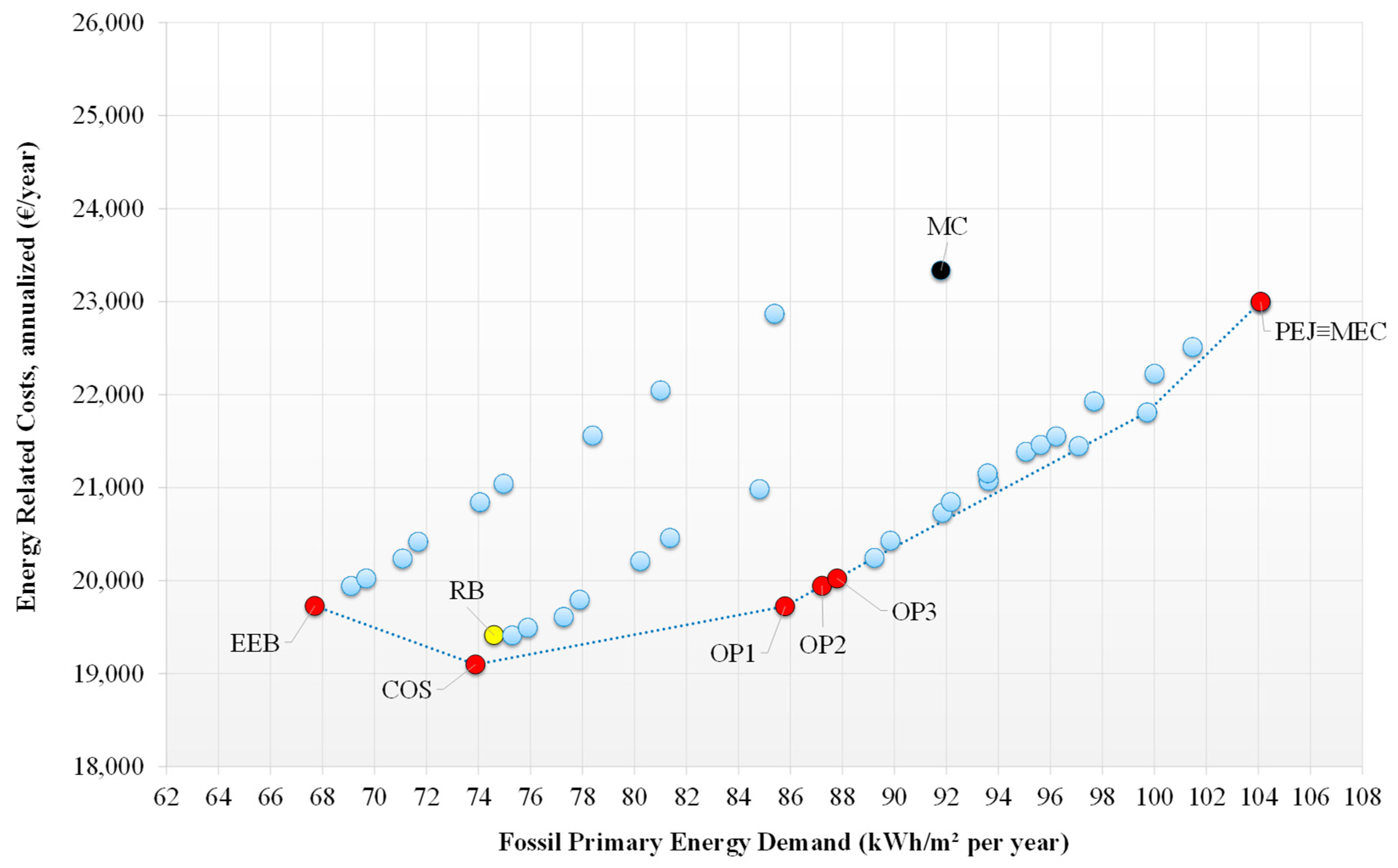
Moving to the climatic zone F, as shown in Figure 4, a different trend of the points depicting the several EEMs was detected. It seems that a major number of cases were analyzed when compared to the warm location, actually for the latter, some points are very close and tend to overlap due to the lower primary energy demands. The colder climatic zone involves greater heating requirements, consequently a noticeable increment of the net primary energy demand determined higher annualized energy-related costs. Consequently, for this case, the cost-optimal solution looks toward measures with reduced energy requirements. This effect is further amplified due to the scarce employment of the renewable sources related to the limited solar irradiance availability, and scarce PV production as a consequence, and the outdoor air temperatures that affect negatively the heat pump’s performance in the winter. Comparison with Figure 3 shows a consistent limitation of the gap between the COS and the RB points. Nevertheless, in comparison with the warm location, the minimal energy performance levels determined a worsening of both the energy and economic scenarios, detecting a greater primary energy demand of 2.1 kWh/m² and an extra cost of 829 € per year compared to the cost-optimal solution, meaning the minimal energy performance levels should consider insulation thicknesses slightly greater than those currently imposed. In addition, the distance between the EEB and COS points is more limited than that determined for the warm location, with the first producing a reduction of the primary energy demand of 6.2 kWh/m² with an extra cost of 1356 € per year, confirming that the employment of insulated envelopes is suggested to match more closely the cost-effective solutions. The other considered EEMs provided, in every case, worsening results and therefore should not be taken into account. In particular, the worst package of measures is represented by the MEC point, representative of a medium-insulated envelope, with annualized energy-related costs similar to the MC point. Evidently, these building configurations determined a noticeable increment of the running costs that prevail on the reduction of expenses required for these packages. In

Table 11. Detected optimal constructive solutions concerning different EEMs for climatic zone F (VWT, insulation thickness in vertical wall; GST, insulation thickness in the ground slab; SFT, insulation thickness in the second last floor; GS, glazing system).

EEMs	VWT	GST	SFT	GS
PEJ	10 cm	10 cm	10 cm	Double pane
OP1	15 cm	10 cm	15 cm	Double pane
OP2	15 cm	15 cm	15 cm	Double pane
OP3	15 cm	15 cm	15 cm	Triple pane
RB	15 cm	15 cm	18 cm	Triple pane
EEB	20 cm	20 cm	20 cm	Triple pane
MEC	10 cm	10 cm	10 cm	Double pane
MC	20 cm	10 cm	10 cm	Double pane
COS	15 cm	20 cm	20 cm	Triple pane

, the results corresponding to the constructive solutions for each point considered were specified for the respective climatic zone. The only differences between COS and EEB concern the employment of a lower insulation thickness in vertical walls. Window systems equipped with triple pane are required to prevent, this time, excessive thermal losses during winter rather than to limit solar gains in summer. It is worth noticing that OP1 and OP2 allowed for the attainment of annualized energy-related costs limited to values lower than 1000 € per year when compared to COS, despite the employment of double pane windows. In addition, OP3 considered the same insulation thicknesses as OP2 but involving triple pane windows; however, the economic and energy scenarios worsened further, meaning that in this location the best compromise between thermal losses and solar gains also has to be identified.

4.2. Cost-Optimal Analysis with Macroeconomic Projection

The same calculations were repeated for the localities by adopting the macroeconomic projection. It is clear that the point distribution is similar to the prior cases, however, a noticeable limitation of the annualized energy-related cost gap was detected. This limitation is due mainly to two factors:

• The more limited EEMs cost due to the exclusion of taxes,
• The lower annualized energy-related costs according to electricity prices considered without VAT and excises.

These effects prevail on the reduction of the discount rate that, conversely, produced greater annualized energy-related costs compared to the financial scenario when projected to the initial year. The combination of these items determined a downshift more or less constant for all of the EEMs, however, few differences among the points’ position can be observed due to the different CO₂ emission costs among the investigated interventions. In Figure 5, the results of the macroeconomic projection are shown for the warm location, whereas

Table 12. CO₂ emissions and corresponding cost for the EEMs considered and comparison between the annualized energy-related costs (AERC) determined for the financial and macroeconomic projections in the warm location.

	CO2 Emissions (Tonnes/Year)	CO2 Emission Cost (€/Year)	Macroeconomic AERC (€/Year)	Financial AERC (€/Year)	Difference Macro/Financial (€/Year)
PEJ	33.3	666	8841	13,745	−4904
OP1	31.4	627	8490	13,229	−4739
OP2	30.5	610	8396	13,105	−4709
OP3	25.3	507	9001	14,390	−5389
RB	27.0	540	9360	14,933	−5573
EEB	22.9	458	10,024	16,272	−6248
MEC	33.4	668	9009	14,030	−5021
MC	25.8	516	10,500	16,940	−6440
COS	29.1	583	8319	13,034	−4715

lists for the more representative packages the annual CO₂ emission, their costs, energy-related costs of financing and macroeconomic projections highlighting the differences. The deviance of the annualized energy-related costs between EEB and MEC, representing respectively, the better and the worst EEM from the point of view of energy consumption and CO₂ emission, is only 210 € per year. Therefore, the inclusion of the CO₂ emission costs in this location did not affect the results noticeably. Indeed, the CO₂ emissions in the formation of the annualized energy-related cost contribute from a minimum of 4.5% to a maximum of 7.5%; however, they did not modify the optimal building configuration and the point distribution. Nevertheless, expensive EEMs producing limited running costs, for instance MC, EEB and RB, provided higher differences between the two projections, meaning a major role of interventions cost compared to the running cost. Consequently, the results of the macroeconomic scenario are more precautionary in presence of buildings with high-energy performances that do not match the cost-optimal solution. Conversely, the differences decrease compared to the two cost-effective interventions and the minimum gap that was detected with OP2. Clearly, the macroeconomic scenario highlighted a consistent reduction of the cost gap between RB and COS, passing to 1000 € when compared with the financial projection (−45%). Nevertheless, in the warm location, the cost-optimal solution provided with the macroeconomic projection, also in this case, did not match the minimal energy performance levels, therefore the latter should be revised for the considered building typology.

The same evaluations were carried out for the building located in the cold location, as depicted in Figure 6; it is clear that the macroeconomic scenario produced a more evident limitation in the cost gap between the RB and the COS points, now separated by 300 € per year with a percentage deviation of 62%, when compared with the financial projection. Effectively, the latter confirms that minimal energy performance levels seem to be developed not far from the cost-optimal solution but exclusively for cold climatic context. In

Table 13. CO₂ emissions and corresponding cost for the EEMs considered and comparison between the annualized energy-related costs (AERC) determined for the financial and macroeconomic projections in the cold location.

	CO2 Emissions (Tonnes/Year)	CO2 Emission cost (€/Year)	Macroeconomic AERC (€/Year)	Financial AERC (€/Year)	Difference Macro/Financial (€/Year)
PEJ	96.3	1926	22,998	35,306	−12,308
OP1	79.4	1588	19,724	30,429	−10,705
OP2	80.7	1614	19,945	30,749	−10,804
OP3	81.3	1625	20,024	30,861	−10,837
RB	70.3	1407	19,413	30,686	−11,273
EEB	62.7	1253	19,729	31,213	−11,484
MEC	96.3	1926	22,998	35,306	−12,308
MC	79.0	1581	22,869	36,604	−13,735
COS	68.4	1368	19,098	29,857	−10,759

, the emitted CO₂ and corresponding costs are listed, as well as a comparison between the annualized energy-related costs determined for the two economic scenarios. The colder climatic context, due to the major heating requirements, made the role of CO₂ emission cost more influential, with an average percentage of 8% of the annualized energy-related cost. In this case, the running cost is augmented and significant for the quantification of the deviances between the financial and macroeconomic projection, as demonstrated by the EEMs with the greatest energy consumptions (MEC and PEJ). OP1 becomes the solution that allows for minimizing the gap between financial and macroeconomic projections.

5. Conclusions

The cost-optimal analysis was used to design a new multistory building in two contrasting climatic zones of the Mediterranean area in order to identify the best building envelope configurations. The latter designed to verify the current regulations in terms of energy performance levels for the climatic zones considered were used as benchmarks (RB). The main investigated parameters concern the insulation thickness in the dispersing opaque walls and the windowed system, with an unvaried air-conditioning plant to meet regulation constraints on the integration of renewable systems in buildings. The analyses were carried out by a financial approach (for private investors) and a macroeconomic projection (to plan regulations) by highlighting the differences among the detected optimal measures. Mainly, financial and macroeconomic projections provided the same cost-optimal solutions. Nevertheless, with a macroeconomic projection, the RB matches the cost-optimal solution only in the cold location, whereas in the warm climatic zone a noticeable deviance was detected and a less insulated envelope equipped with triple pane systems is recommended. In particular, a scarcely insulated ground floor allows for the transfer of thermal power to the soil during summer, limiting the cooling requirements. Furthermore, lower insulation thicknesses in vertical opaque walls equipped with triple pane windows represent at an annual level the best compromise between thermal losses and employment of solar gains. Consequently, in the warm location, the minimal energy performance levels set for the RB should be revised, because less insulated building configurations allow for a reduction of the initial investment that prevails on a slight augmentation of the running costs. Regarding the cold climate, the macroeconomic projection produced a noticeable reduction of the cost gap between RB and the cost-optimal solution, however, a combination of measures that further reduce the thermal losses through the envelope are suggested. Nevertheless, the results confirm the good agreement between the measures imposed by regulation and the cost-effective solution.

The cost-optimal analyses carried out by the financial projection highlighted a major gap between the RB and cost-optimal solutions, especially for the warm location. In particular, the RB showed a greater annualized energy-related cost increment. Therefore, from the perspective of private investors, a further distance growth between the two points, equal to 859 € per year, 82% higher than the macroeconomic scenario, was detected. The role of the CO₂ emission on the points’ distribution is marginal, by considering that the annualized energy-related costs varied between 4.5% and 7.5%. This is due to the favorable application of renewable systems connected with the advantageous climatic conditions. In the cold location, a distance growth between RB and the cost-optimal solution was detected again, this time at 514 € per year (+ 163%). However, the role of the CO₂ is more significant with an average weight of 8% on the global costs, due to the greater energy consumptions for heating. When the distance of the points denoting the several combination of measures is compared between the two economic projections, the deviances were more evident in the presence of expensive interventions in the warm location, denoting a greater role of the investment costs than the running costs. Conversely, the greatest deviances were detected also in correspondence to interventions with large energy consumption in the cold location, due to the major role of the CO₂ emissions. Globally, the financial projection tends to provide results close to the macroeconomic projection in warm climatic zones or in the presence of a high percentage of primary energy covered by renewable sources. However, the macroeconomic scenario returns a more limited distance between the minimal energy performance levels and the cost-optimal solutions, therefore it is far from the real economic frame sustained by private investors.

Despite the regulations being susceptible to further improvements, especially in warm climates, the results produced by the two projections confirm the possibility to design highly efficient buildings in the context of a sustainable economic frame. Regarding the required costs, the role of the renewable systems is marginal when compared with the other items, producing beneficial effects on the environmental impact point of view. In this way, the cost-optimal analysis can support the diffusion of more sustainable edifices because it is confirmed that use of this tool can effectively limit energy consumption in buildings and increase benefits for the society. Therefore, this approach is highly recommended in countries where directives concerning building energy performances are not yet promulgated.