A Reliability-Based Network Reconfiguration Model in Distribution System with DGs and ESSs Using Mixed-Integer Programming

Abstract

Widely used distribution generations (DGs) and energy storage systems (ESSs) enable a distribution system to have a more flexible fault reconfiguration capability. In order to enhance the service reliability and the benefit of distribution networks with DGs and ESSs, this paper proposes a novel distribution system reconfiguration (DSR) model including DGs and ESSs. Meanwhile, the impact of sectionalizing switches and tie switches on reliability is considered. The concept of “boundary switch” is introduced for quantifying the customer interruption duration. The DSR model is presented to minimize the sum of the customer interruption cost, the operation cost of switches, and the depreciation cost of DGs and ESSs. Furthermore, the proposed model is converted into a mixed-integer linear programming, which can be efficiently solved by commercial solvers. Finally, the validity and efficiency of the proposed DSR model are verified by a modified IEEE 33-bus system and a modified PG&E69-bus network. The obtained results indicate the advantages of DGs and ESSs in reducing outage time, and suggest that the types and locations of SSs have great effects on the resulting benefit of DGs and ESSs.

1. Introduction

Due to a shortage of resources and the pressure arising from environmental degradation, the government has increased its demands for energy savings and carbon emissions reductions. Distributed generations (DGs) [1,2], as flexible and usually environmentally friendly sources, have attracted the attention of electric utilities. Moreover, customers have more strict demands for service quality. Energy Storage Systems (ESSs) and DGs could restore power supply to affected customers when the distribution network is separated from the upper power grid due to a failure, which would improve the reliability and resilience of system [3,4]. Therefore, ESSs and DGs play an important role in restoring more customers in distribution system reconfiguration (DSR). At the same time, sectionalizing switches (SSs) and tie switches (TSs) can change the structure of a distribution network during reconfiguration [5], which would have a direct impact on the reliability of the overall system. In this regard, it is worthwhile to conduct a reliability-based method of DSR considering DGs, ESSs, and SSs, which is the focus of this paper.

DGs can be sorted into dispatchable and nondispatchable DGs according to whether they have black start capability. Nondispatchable DGs with intermittent output cannot regulate the frequency and voltage, thus they are unable to provide a reliable power supply during outages [6]. ESSs not only provide both technical services and economic benefits [7], but also play an important role in the service restoration. On the other hand, the areas that can be restored by ESSs are restricted due to the capacity and power limits of ESSs. SSs, which consist of remote-controlled switches (RCSs) and manual switches (MSs), are utilized to isolate failures and reduce the interruption duration of customers. Additionally, RCSs isolate failures with a shorter actuation time than MSs [8]. Thus, the customer interruption duration is related to the locations of RCSs, MSs, DGs, and ESSs. All these could pose great challenges for system operators during the process of reconfiguration.

Finding the best network topology considering the power losses, energy demand, voltage profile, and operational performance is the core of the DSR problem [9]. Various solution algorithms regarding DSR have been proposed in the literature. Generally, there are two well-known methods to solve the DSR problem: heuristic algorithms and classical optimization methods. In [10,11,12], the Genetic Algorithm (GA) was utilized to solve the network reconfiguration problem. The authors of [13] presented a multi-objective algorithm to solve stochastic DSR problem for systems with distributed wind power generation and fuel cells and used the particle swarm optimization (PSO) method. The authors of [14] introduced an ant colony search algorithm (ACSA) to solve DSR with joint consideration of the optimal placement of capacitors. In addition, the authors of [15] presented a Benders decomposition approach that in the first stage determined the radial topology of networks and in the second stage determined the feasibility of the master problem solution by means of optimal power flow. The authors of [16,17,18] developed a mixed-integer programming (MIP) for the DSR problem. The authors of [19] derived a set of linear current flow equations and then formulated the DSR problem for loss minimization as an MIP model.

In particular, DGs and ESSs can restore power to local loads and improve the operational performance of networks during outages—benefits that have attracted the attention of researchers. The model described in [20] presented a method for determining the minimum loss configuration in distribution networks with uncertain load and DGs. The authors of [21] proposed a multi-objective approach for network reconfiguration with optimal DG power factor. The DSR problem with DGs was presented in [22,23] to minimize real power loss and improve voltage profile. In [24], the authors employed a DSR model for the network losses in MIP formulation while DG locations and sizes are simultaneously optimized. The studies in [6] developed a model for the optimal siting and sizing of ESSs embedding network reconfiguration. The model described in [25] presented a new energy management strategy for minimizing operational cost in DSR considering DGs and ESSs. In [9], wind energy and ESSs were applied to improve system reliability, and the best reconfiguration topology was found by determining the best switching sequence.

As pointed out earlier, DSR can be accomplished via the reconfiguration of SSs and TSs. It makes sense to consider DGs, ESSs, SSs, and TSs simultaneously in DSR, to which little attention has been paid, but it should not be ignored. However, the areas that can be recovered by means of DGs and ESSs are restricted because of the power limit of DGs and ESSs and the battery capacity limit of ESSs. The healthy areas are determined through switching actions, so the types and locations of SSs play a crucial role in the reconfiguration process. All of these factors make it difficult to determine the customer interruption time. This paper proposes a novel DSR model considering DGs and ESSs; the main contributions are as follows:

• DGs and ESSs are considered together in order to increase power supply reliability during service outages. Additionally, DGs without the function of black start cannot supply power independently in the service restoration, which is also taken into account in this paper. A radial configuration model is also introduced to ensure that the network topology is radial.
• The types and locations of SSs have great effects on the benefit of the distribution system with DGs and ESSs. This paper considers the impact of DGs, ESSs, SSs, and TSs on the system service reliability. Furthermore, the customer interruption duration is quantified based on the proposed “boundary switch.”
• The proposed method is mathematically formulated as an MIP model, which provides an efficient framework for the incorporation of DGs and ESSs in DSR. Additionally, the MIP model with the valuable property in terms of solution quality can be easily solved via off-the-shelf software.

The remainder of this paper is organized as follows. The problem statement is put forward in Section 2. Section 3 describes the formulation of the proposed DSR model, with details of the “boundary switch” introduced. The case studies as well as the obtained results are presented in Section 4. Finally, conclusions are drawn in Section 5.

2. Problem Statement

The model for network reconfiguration in distribution system with DGs and ESSs is formulated by considering the following assumptions:

(1)

TSs that connect/disconnect neighboring feeders for enhancing reliability are considered as automatic switches.

(2)

For the sake of simplicity, this paper assumes that SSs are all installed at the beginning of each branch, and their malfunctioning probability is ignored.

(3)

The loss of ESSs during discharge is ignored.

It is worth mentioning that the DG without the function of black start only can be used with other reliable power sources, such as the main power, neighboring feeders, ESSs, and DGs with the function of black start. A sample network equipped with one DG, one ESS, and SSs is depicted in Figure 1. The DG at node 10 has the capability of black start supposing a fault occurs in branch 2–3.

First of all, the circuit breaker at the beginning of the feeder trips and all load are de-energized. Then system operators will open the RCS on branches 2–3 and 7–8 and close TS remotely, so that load points (LPs) 1–2 and 8 can be restored promptly. Hence, the interruption duration of LPs 1–2 and 8 is the automatic switching time. When the power generation of DG exceeds the total load demands of LPs 9–10, LPs 9–10 can be isolated from the fault area and restored via opening the MS on branch 4–9. Similarly, if the power generation of ESS exceeds the total load demands of LPs 11–12, LPs 11–12 can be restored through opening the MS on branch 6–11. The interruption duration of LPs 9–12 is the manual switching time. LPs 3–7 would be interrupted until the fault is repaired. Therefore, the interruption duration of LPs 3–7 is the fault repairing time.

From the analysis above, it can be seen that (1) the distribution network has formed four independent power supply areas with SSs as the boundaries through switching actions, and the four areas are maintained by the main power, neighboring feeder, ESS, and DG, respectively; (2) DGs and ESSs can restore power to the local loads and reduce outage time after the fault occurs; and (3) the locations of SSs, DGs, and ESSs have great effects on the customer interruption duration.

3. Network Reconfiguration Model

3.1. Basic Concept

In order to satisfy the radial structure of distribution networks after reconfiguration, this paper introduces the concepts of “virtual node 0” and virtual branches, so as to strictly guarantee the radial topology of networks.

The “virtual node 0” is independent of distribution networks; it does not have load demand and actual power output. Virtual branches formed by connecting “virtual node 0” with the main source, neighboring feeders, DGs that have the black-start function, and ESSs. Virtual branches do not transmit actual power and have an open or closed status. Taking the simple network described in Section 2 as an example, the network structure after adding “virtual node 0” and virtual branches is depicted in Figure 2 as follow:

3.2. Formulation

3.2.1. Objective Function

The objective function of the proposed DSR model has three parts, the customer interruption cost, the operation cost of switches, and the depreciation cost of DGs and ESSs, and is expressed as follows:

$$\begin{array}{l}\mathbf{Minimize}\mathrm{COST}={\displaystyle \sum _{n\in {\mathsf{\Omega }}_{\mathrm{load}}}{P}_n{t}_n{e}_{unit}}+{\displaystyle \sum _{ij\in {\mathsf{\Omega }}_{\mathrm{switch}}}{C}_{switch}(1-{\alpha }_{ij})}+{\displaystyle \sum _{ij\in {\mathsf{\Omega }}_{\mathrm{tie}}}{C}_{switch}{\alpha }_{ij}}\\ +{\displaystyle \sum _{i\in {\mathsf{\Omega }}_{\mathrm{DG}}}{C}_{dep,dg}{P}_{i,dg}+{\displaystyle \sum _{n\in {\mathsf{\Omega }}_{\mathrm{ESS}}}{C}_{dep,ess}E{P}_n}}\end{array}$$

(1)

The first term represents the customer interruption cost. The outage cost is determined by the actual load demand, the customer interruption time, and the unit interruption cost. The second and third terms are the operational costs of SSs and TSs, respectively. It is worth mentioning that the operational cost of switches is utilized to decrease the number of switching operations in DSR. The fourth and fifth terms are the depreciation costs of DGs and ESSs, respectively.

3.2.2. Constraints

(1) The operating state of branch.

When the branch is not equipped with a SS, the branch is closed. In particular, the virtual branches that were formed by connecting “virtual node 0” with the main source and neighboring feeders would remain closed. The virtual branches that were formed by connecting “virtual node 0” with ESSs and DGs that have black start have two possible statuses (open/closed).

$$\{\begin{array}{l}{\alpha }_{ij}\le 1\begin{array}{cc}& ij\in {\mathsf{\Omega }}_{\mathrm{con}}\end{array}\\ {\alpha }_{ij}=1\begin{array}{cc}& ij\in {\mathsf{\Omega }}_{\mathrm{non}}\end{array}\end{array}$$

(2)

The set Ω_con includes the branches equipped with SSs, the virtual branches that were formed by connecting “virtual node 0” with ESSs, and DGs that have black start. The remaining branches are included in Ω_non.

(2) Radial configuration.

Generally, the distribution network is operated in the radial structure. The spanning tree approach used in [17] is introduced to ensure the radial structure of network after reconfiguration.

$${LL}_{ij}+R{R}_{ij}={\alpha }_{ij}$$

(3)

$${\displaystyle \sum _{k0\in {\mathsf{\Omega }}_{in,0}}{LL}_{k0}}+{\displaystyle \sum _{0j\in {\mathsf{\Omega }}_{out,0}}R{R}_{0j}}=0$$

(4)

$${\displaystyle \sum _{ki\in {\mathsf{\Omega }}_{in,i}}{LL}_{ki}}+{\displaystyle \sum _{ij\in {\mathsf{\Omega }}_{out,i}}R{R}_{ij}}\le 1$$

(5)

$${\displaystyle \sum _{ki\in {\mathsf{\Omega }}_{in,i}}{LL}_{ki}}+{\displaystyle \sum _{ij\in {\mathsf{\Omega }}_{out,i}}R{R}_{ij}}\ge X_i$$

(6)

Equation (3) indicates the relationship between the spanning tree variables and the operating state of the branch. The network is represented as a spanning tree originating from “virtual node 0.” That is to say, “virtual node 0” does not have a parent node, as shown in Equation (4). Except for “virtual node 0,” the rest have only one parent node when they are charged, as shown in Equations (5) and (6).

However, Equations (3)–(6) still cannot guarantee that a ring structure network would not appear after reconfiguration. Therefore, “virtual demand” is proposed to resolve this situation. Each energized node after reconfiguration has one unit of “virtual demand.” The virtual power is only provided by “virtual node 0.” The virtual demand transmission paths consist of real power supply branches as well as virtual branches.

$$X_i{f}_{Li}+{\displaystyle \sum _{ij\in {\mathsf{\Omega }}_{out,i}}{f}_{ij}}-{\displaystyle \sum _{ki\in {\mathsf{\Omega }}_{in,i}}{f}_{ki}}=0$$

(7)

$$-{\alpha }_{ij}N\le f_{ij}\le {\alpha }_{ij}N$$

(8)

(3) Branch-Node state.

$${\alpha }_{ij}-1\le X_i-X_j\le 1-{\alpha }_{ij}$$

(9)

Equation (9) ensures that the status of nodes at both ends of the branch is consistent when the branch is closed.

(4) Power balance of node.

$$X_i{P}_i-P_{i,dg}-P_{i,ess}+{\displaystyle \sum _{ij\in {\mathsf{\Omega }}_{out,i}}{P}_{ij}}-{\displaystyle \sum _{ki\in {\mathsf{\Omega }}_{in,i}}{P}_{ki}}=0$$

(10)

$$X_i{Q}_i-Q_{i,dg}-Q_{i,ess}+{\displaystyle \sum _{ij\in {\mathsf{\Omega }}_{out,i}}{Q}_{ij}}-{\displaystyle \sum _{ki\in {\mathsf{\Omega }}_{in,i}}{Q}_{ki}}=0$$

(11)

Equations (10) and (11) represent the active and reactive power balance at node i. It should be noted that the load demand of the node located at the end of the faulted branch is assumed to be infinite, which is used to determine that the branch has a three-phase short-circuit fault.

(5) Power output limits of DG.

$$0\le P_{i,dg}\le X_i{S}_{i,dg}\begin{array}{cc}& \forall i\in {\mathsf{\Omega }}_{\mathrm{DG}}\end{array}$$

(12)

$$-X_i{S}_{i,dg}\le Q_{i,dg}\le X_i{S}_{i,dg}\begin{array}{cc}& \forall i\in {\mathsf{\Omega }}_{\mathrm{DG}}\end{array}$$

(13)

$$P_{i,dg}^2+Q_{i,dg}^2\le S_{i,dg}^2\begin{array}{cc}& \forall i\in {\mathsf{\Omega }}_{\mathrm{DG}}\end{array}$$

(14)

The power output limits of DGs are shown in Equations (12) and (13). The apparent power flow limit of DGs is represented in Equation (14).

(6) Power output limits of ESS.

$$0\le P_{i,ess}\le X_i{S}_{i,ess}\begin{array}{cc}& \forall i\in {\mathsf{\Omega }}_{\mathrm{ESS}}\end{array}$$

(15)

$$-X_i{S}_{i,ess}\le Q_{i,ess}\le X_i{S}_{i,ess}\begin{array}{cc}& \forall i\in {\mathsf{\Omega }}_{\mathrm{ESS}}\end{array}$$

(16)

$$P_{i,ess}^2+Q_{i,ess}^2\le S_{i,ess}^2\begin{array}{cc}& \forall i\in {\mathsf{\Omega }}_{\mathrm{ESS}}\end{array}$$

(17)

Equations (15) and (16) limit the power output of ESSs. The apparent power flow limit of ESSs is represented in Equation (17).

(7) Power limits of branch.

$$-{\alpha }_{ij}{S}_{ij,max}\le P_{ij}\le {\alpha }_{ij}{S}_{ij,max}$$

(18)

$$-{\alpha }_{ij}{S}_{ij,max}\le Q_{ij}\le {\alpha }_{ij}{S}_{ij,max}$$

(19)

$$P_{ij}^2+Q_{ij}^2\le S_{ij,max}^2$$

(20)

The active and reactive power flow limits of branch i–j are given in Equations (18) and (19). The apparent power flow limit of branch i–j is considered in Equation (20). It should be noted that Equations (14), (17), and (20) include quadratic square terms that can be linearized with the approach applied in [19].

3.2.3. Boundary Switch

As pointed out in Section 2, SSs can isolate the failure from the network by switching actions, and the distribution system is divided into several isolated healthy areas with SSs as boundaries. Therefore, the concept of “boundary switch” is proposed in this paper. If a fault occurs in the network, load n can be restored by changing the status of some specific switches, then these switches are called the boundary switch of load n. Taking the distribution network in Figure 1 as an example, the MS on branch 4–9 is the boundary switch of LPs 9–10; the MS on branch 6–11 is the boundary switch of LPs 11–12; the RCS on branch 2–3 is the boundary switch of LPs 1–2; and the RCS on branch 7–8 is the boundary switch of LP 8.

The switch on branch ij is whether the boundary switch of load n, depends on the operational status of itself and the switches on the shortest path that between the branch ij and the load n. If all the switches on the shortest path stay closed but the switch is opened, then the switch on branch ij is the boundary switch of load n. The boundary switch can be identified as follows.

$$\frac{{\displaystyle \sum _{km\in {\mathsf{\Omega }}_{ij,n}}(1-{\alpha }_{km})}}{M}\le C_{ij,n}\le {\displaystyle \sum _{km\in {\mathsf{\Omega }}_{ij,n}}(1-{\alpha }_{km})}\begin{array}{cc}& \forall n\in {\mathsf{\Omega }}_{\mathrm{load}},\end{array}ij\in {\mathsf{\Omega }}_{\mathrm{switch}}$$

(21)

$$H_{ij,n}^{}=(1-{\alpha }_{ij})(1-C_{ij,n})\begin{array}{cc}& \forall n\in {\mathsf{\Omega }}_{\mathrm{load}},\end{array}ij\in {\mathsf{\Omega }}_{\mathrm{switch}}$$

(22)

In Equation (21), Ω_ij,n represents the set of branches equipped with SSs on the shortest path from the branch ij to the load n. When the switches in Ω_ij,n do not act, and all branches of Ω_ij,n remain closed, C_ij,n is forced to get 0; otherwise, C_ij,n is equal to 1. Equation (22) ensures that H_ij,n = 1 only when α_ij = 0 and C_ij,n = 0. In other words, the switch on branch ij is the boundary switch of load n only when all the switches in Ω_ij,n do not act but itself actions. Furthermore, Equation (22) can be linearized as follows:

$$H_{ij,n}\le 1-{\alpha }_{ij}\begin{array}{cc}& \forall n\in {\mathsf{\Omega }}_{\mathrm{load}},ij\in {\mathsf{\Omega }}_{\mathrm{switch}}\end{array}$$

(23)

$$H_{ij,n}\le 1-C_{ij,n}\begin{array}{cc}& \forall n\in {\mathsf{\Omega }}_{\mathrm{load}},ij\in {\mathsf{\Omega }}_{\mathrm{switch}}\end{array}$$

(24)

$$H_{ij,n}\ge 1-{\alpha }_{ij}-C_{ij,n}\begin{array}{cc}& \forall n\in {\mathsf{\Omega }}_{\mathrm{load}},ij\in {\mathsf{\Omega }}_{\mathrm{switch}}\end{array}.$$

(25)

3.2.4. Energy Storage System

Utilities are trying to take advantage of ESSs to reduce outage time. Due to the energy storage in ESSs being limited, the number of customers supplied by ESSs is closely related to the discharging time of ESSs. It can be concluded that the discharging time of ESS located on load n depends on the maximum switching time of the boundary switch of load n. Therefore, the discharging time of ESS can be classified into three types: 0, t^rep − t^manu, and t^rep − t^auto. The binary variables $G_{n,ess}^{MS}$ and $G_{n,ess}^{RCS}$ are used to determine the discharging time types of ESS located on node n.

$$\frac{{\displaystyle \sum _{ij\in {\mathsf{\Omega }}_{\mathrm{MS}}}{H}_{ij,n}}}{M}\le G_{n,ess}^{MS}\le {\displaystyle \sum _{ij\in {\mathsf{\Omega }}_{\mathrm{MS}}}{H}_{ij,n}}\begin{array}{cc}& \forall n\in {\mathsf{\Omega }}_{\mathrm{ESS}}\end{array}$$

(26)

$$\frac{({\displaystyle \sum _{ij\in {\mathsf{\Omega }}_{\mathrm{RCS}}}{H}_{ij,n})(1-G_{n,ess}^{MS})}}{M}\le G_{n,ess}^{RCS}\le ({\displaystyle \sum _{ij\in {\mathsf{\Omega }}_{\mathrm{RCS}}}{H}_{ij,n})(1-G_{n,ess}^{MS})}\begin{array}{cc}& \forall n\in {\mathsf{\Omega }}_{\mathrm{ESS}}\end{array}$$

(27)

Equation (26) ensures $G_{n,ess}^{MS}$ = 1 when at least one boundary switch of load n is MS; otherwise, $G_{n,ess}^{MS}$ = 0. In Equation (27), when the binary variable $G_{n,ess}^{MS}$ = 1, the value of $G_{n,ess}^{RCS}$ is 0 whether or not one boundary switch of load n is RCS. Furthermore, Equation (27) can be linearized as follows:

$$G_{n,ess}^{RCS}-{\displaystyle \sum _{ij\in {\mathsf{\Omega }}_{\mathrm{RCS}}}{H}_{ij,n}}\le M\cdot G_{n,ess}^{MS}\begin{array}{cc}& \forall n\in {\mathsf{\Omega }}_{\mathrm{ESS}}\end{array}$$

(28)

$$G_{n,ess}^{RCS}-\frac{{\displaystyle \sum _{ij\in {\mathsf{\Omega }}_{\mathrm{RCS}}}{H}_{ij,n}}}{M}\ge -M\cdot G_{n,ess}^{MS}\begin{array}{cc}& \forall n\in {\mathsf{\Omega }}_{\mathrm{ESS}}\end{array}$$

(29)

$$-M(1-G_{n,ess}^{MS})\le G_{n,ess}^{RCS}\le M(1-G_{n,ess}^{MS})\begin{array}{cc}& \forall n\in {\mathsf{\Omega }}_{\mathrm{ESS}}\end{array}.$$

(30)

The energy provided by the ESS located on node n during the repair time can be expressed as follows:

$$E{P}_n=P_{n,ess}{t}_n=P_{n,ess}(t^{rep}-t^{manu})G_{n,ess}^{MS}{X}_n+P_{n,ess}(t^{rep}-t^{auto})G_{n,ess}^{RCS}{X}_n\begin{array}{cc}& \forall n\in {\mathsf{\Omega }}_{\mathrm{ESS}}\end{array}$$

(31)

$$E{P}_{n,0}-P_{n,ess}{t}_n\ge 0\begin{array}{cc}& \forall n\in {\mathsf{\Omega }}_{\mathrm{ESS}}\end{array}.$$

(32)

In Equation (31), the first term indicates that the discharging time of ESS is t^rep − t^manu; the second term indicates that the discharging time of ESS is t^rep − t^auto. In particular, when the ESS does not discharge, namely X_n = 0, EP_n will be forced to 0. Equation (32) represents that the energy storage level of ESS cannot be negative. Note that Equation (31) is a complex expression and can be linearized through introducing ancillary variables and equivalent conversion as follows:

$$N_{n,ess}^{MS}=G_{n,ess}^{MS}{X}_n\begin{array}{cc}& \forall n\in {\mathsf{\Omega }}_{\mathrm{ESS}}\end{array}$$

(33)

$$N_{n,ess}^{MS}\le G_{n,ess}^{MS}\begin{array}{cc}& \forall n\in {\mathsf{\Omega }}_{\mathrm{ESS}}\end{array}$$

(34)

$$N_{n,ess}^{MS}\le X_n\begin{array}{cc}& \forall n\in {\mathsf{\Omega }}_{\mathrm{ESS}}\end{array}$$

(35)

$$N_{n,ess}^{MS}\ge G_{n,ess}^{MS}+X_n-1\begin{array}{cc}& \forall n\in {\mathsf{\Omega }}_{\mathrm{ESS}}\end{array}$$

(36)

$$P_{n,ess}^{MS}=P_{n,ess}{N}_{n,ess}^{MS}\begin{array}{cc}& \forall n\in {\mathsf{\Omega }}_{\mathrm{ESS}}\end{array}$$

(37)

$$0\le P_{n,ess}^{MS}\le S_{n,ess}{N}_{n,ess}^{MS}\begin{array}{cc}& \forall n\in {\mathsf{\Omega }}_{\mathrm{ESS}}\end{array}$$

(38)

$$P_{n,ess}-S_{n,ess}(1-N_{n,ess}^{MS})\le P_{n,ess}^{MS}\le P_{n,ess}\begin{array}{cc}& \forall n\in {\mathsf{\Omega }}_{\mathrm{ESS}}\end{array}$$

(39)

$$N_{n,ess}^{RCS}=G_{n,ess}^{RCS}{X}_n\begin{array}{cc}& \forall n\in {\mathsf{\Omega }}_{\mathrm{ESS}}\end{array}$$

(40)

$$N_{n,ess}^{RCS}\le G_{n,ess}^{RCS}\begin{array}{cc}& \forall n\in {\mathsf{\Omega }}_{\mathrm{ESS}}\end{array}$$

(41)

$$N_{n,ess}^{RCS}\le X_n\begin{array}{cc}& \forall n\in {\mathsf{\Omega }}_{\mathrm{ESS}}\end{array}$$

(42)

$$N_{n,ess}^{RCS}\ge G_{n,ess}^{RCS}+X_n-1\begin{array}{cc}& \forall n\in {\mathsf{\Omega }}_{\mathrm{ESS}}\end{array}$$

(43)

$$P_{n,ess}^{RCS}=P_{n,ess}{N}_{n,ess}^{RCS}\begin{array}{cc}& \forall n\in {\mathsf{\Omega }}_{\mathrm{ESS}}\end{array}$$

(44)

$$0\le P_{n,ess}^{RCS}\le S_{n,ess}{N}_{n,ess}^{RCS}\begin{array}{cc}& \forall n\in {\mathsf{\Omega }}_{\mathrm{ESS}}\end{array}$$

(45)

$$P_{n,ess}-S_{n,ess}(1-N_{n,ess}^{RCS})\le P_{n,ess}^{RCS}\le P_{n,ess}\begin{array}{cc}& \forall n\in {\mathsf{\Omega }}_{\mathrm{ESS}}\end{array}$$

(46)

$$E{P}_n=(t^{rep}-t^{manu})P_{n,ess}^{MS}+(t^{rep}-t^{auto})P_{n,ess}^{RCS}\begin{array}{cc}& \forall n\in {\mathsf{\Omega }}_{\mathrm{ESS}}\end{array}.$$

(47)

3.2.5. Customer Interruption Time

According to the formulations in Section 2 and Section 3.2.3, the customer interruption time is related to the maximum switching time of the boundary switch (RCS or MS), as well as whether service can be restored.

$$t_n\ge t^{auto}{H}_{ij,n}\begin{array}{cc}& \forall n\in {\mathsf{\Omega }}_{\mathrm{load}},\end{array}ij\in {\mathsf{\Omega }}_{\mathrm{RCS}}$$

(48)

$$t_n\ge t^{manu}{H}_{ij,n}\begin{array}{cc}& \forall n\in {\mathsf{\Omega }}_{\mathrm{load}},\end{array}ij\in {\mathsf{\Omega }}_{\mathrm{MS}}$$

(49)

$$t_n\ge t^{rep}(1-X_n)\begin{array}{cc}& \forall n\in {\mathsf{\Omega }}_{\mathrm{load}}\end{array}$$

(50)

Equation (48) is used to determine the interruption time of customers who can be isolated from the fault via RCS. Equation (49) is used to determine the interruption time of customers who can be isolated from the fault via MS. Equation (50) describes the interruption time of a customer who would be interrupted until the fault is repaired.

4. Case Studies

The proposed DSR model is implemented in the Python 2.7 [26] environment and solved using the MIP solver CPLEX 12.7 [27] on a 3.4-GHz processor with 8 GB of random-access memory, and the optimality gap of CPLEX is set to 0%. Several case studies are presented to demonstrate the effectiveness of the proposed approach, as well as to show the advantages of considering DGs, ESSs, SSs, and TSs simultaneously in the DSR problem.

4.1. IEEE 33-Bus

The proposed model is first applied to a modified IEEE 33-bus network with five RCSs, 11 MSs, two TSs, four DGs, and one ESS. The network is connected to two neighboring networks, one located on node 34 with a maximum reserve apparent power generation of 350 kVA; another is located on node 35 and the maximum reserve apparent power generation is 700 kVA. The locations of SSs and the parameters of DGs are shown in

Table 1. The locations of SS.

Types of SSs	Locations
RCS	2–3, 5–6, 8–9, 13–14, 28–29
MS	3–4, 6–7, 7–8, 10–11, 14–15, 16–17, 19–20, 24–25, 26–27, 30–31, 31–32

and

Table 2. DG parameters.

Unit	Whether It Can Black-Start	Rated Apparent Power/kVA
DG1	Yes	600
DG2	No	350
DG3	No	500
DG4	Yes	500

, respectively. The modified network is depicted in Figure 3. The load parameters are given in [28]. The unit interruption cost is considered to be $0.60/kWh, and the operating cost of the switch is set equal to $5 at a time. The depreciation costs of DG and ESS are assumed to be $0.05/kW and $0.10/kWh, respectively. The initial energy level and power rating of ESS are considered to be 1 MWh and 1 MVA, respectively. The restoration time associated with RCS and MS is assumed to be 2 min and 1 h, respectively. Additionally, the repair time is assumed to be 3 h.

Supposing a fault occurs in branch 5–6 in Figure 3, to analyze the advantages of distribution network with DGs and ESSs, four cases are simulated as follows:

• Case I: The network is not equipped with any DGs or ESSs;
• Case II: The network is equipped with one ESS;
• Case III: The network is equipped with four DGs;
• Case IV: The network is equipped with four DGs and one ESS simultaneously.

The network reconfiguration results and related costs of Cases I–IV are provided in

Table 3. Simulated results of Cases I–IV.

Case	Closed Switches	Open Switches	Interruption Cost ($)	Total Cost ($)
I	18–34, 33–35	5–6, 14–15, 30–31	2904.20	2929.20
II	18–34, 33–35	5–6, 8–9, 30–31	2026.70	2148.10
III	18–34, 33–35	5–6, 8–9, 28–29,	1213.50	1264.90
IV	18–34, 33–35	5–6, 6–7, 13–14, 28–29	898.80	1025.50

.

According to the results shown in Table 3, the interruption cost of Case I is $2904.20, which is about 223% more than that of Case IV. It is clear that DGs and ESSs could enhance the service reliability. By comparing Cases I and II, the interruption cost of Case II falls to $2026.70 because LPs 9–14 are restored by the ESS installed on node 13. In addition, LP 8 is still interrupted even though there is an MS on branch 7–8. Thus, the number of restorable customers is restricted due to the battery capacity of ESS being limited. In Case III, LPs 9–18 and 29–30 are energized through DG3, DG4, and the neighboring feeders. The interruption cost of the system falls from $2904.20 to $1213.50, a nearly 139% reduction. Hence, DGs make significant contributions to improving the system reliability in DSR. 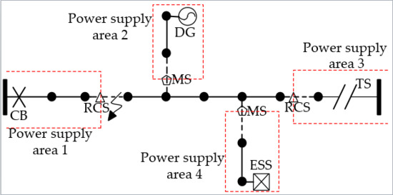The interruption cost of Case IV falls to $898.80, which is the lowest cost in the four cases. Additionally, the network in Case IV has formed four separate power supply areas by switching actions. It can be determined that LPs 2–5, 19–22, and 23–25 are restored through the main power; LPs 7–13 are restored through DG2 and the ESS; LPs 14–18 are restored through DG3 and the neighboring feeder on node 34; and LPs 29–33 are restored through DG4 and the neighboring feeder on node 35. DGs and ESSs are available resources near loads, and can restore power to the affected customers when faults occur, thereby reducing the number of affected customers and improving the service reliability.

Types and locations of SSs: The types and locations of SSs play an important role in the customer interruption time. With this in mind, in Case V, the RCS on branch 28–29 is replaced with an MS. In Case VI, the RCS on branch 28–29 is removed and an RCS is added to branch 29–30. In Case VII, the RCS on branch 28–29 is removed and an MS is added to branch 29–30. The network reconfiguration results and related costs of Cases V–VII are shown in

Table 4. Simulated results of Case V–VII.

Case	Closed Switches	Open Switches	Interruption Cost ($)	Total Cost ($)
V	18–34, 33–35	5–6, 6–7, 13–14, 28–29	1328.00	1454.70
VI	18–34, 33–35	5–6, 6–7, 13–14, 29–30	1112.40	1231.00
VII	18–34, 33–35	5–6, 6–7, 13–14, 29–30	1472.00	1590.60

.

As shown in Table 4, the interruption cost of Case V ($1328.00) is more than that of Case IV ($898.80). This is because MSs have a longer actuation time than RCSs, so the outage time of LPs 29–33 increases and the interruption cost of system increases. In addition, the interruption cost of Case VI is $213.60 more than that of Case IV. This is because the RCS on branch 28–29 is removed; LP 29 cannot be restored via DG4 and would be interrupted until the fault is repaired. By comparison with Case IV–VII, the interruption cost of Case VII is $1472.00, which is the highest cost in Case IV–VII. It seems that the reliability of system can be improved by equipping important loads with more SSs. Based on the results, it can be concluded that the types and locations of SSs would affect the recovery area and performance of DGs in DSR.

Initial energy and power rating of ESS: It is clear that the initial energy and power rating of ESSs play an important role in the performance of ESSs in DSR. In this regard, the initial energy level of ESS on node 13 is changed to 0.5 MWh, and considered as Case VIII; in Case IX, the power rating of ESS on node 13 is changed to 0.4 MVA. The reconfiguration results and relevant costs of Cases VIII–IX are provided through

Table 5. Simulated results of Case VIII–IX.

Case	Closed Switches	Open Switches	Interruption Cost ($)	Total Cost ($)
VIII	18–34, 33–35	5–6, 6–7, 28–29	1125.00	1196.40
IX	18–34, 33–35	5–6, 6–7, 28–29	1125.00	1196.40

.

Table 5 shows that the network reconfiguration result of Case VIII is the same as that of Case IX, LPs 7–18 are restored through DG2, DG3, ESS, and the neighboring feeders on node 34. By a comparison of Case IV and Case VIII, it can be determined that the interruption time of LPs 14–18 in Case IV is the automatic switching time, while the interruption time of LPs 14–18 in Case VIII is the manual switching time, resulting in an increase in the outage cost. This means that ESSs would influence the performance of DGs because ESSs play a similar role to DGs in DSR. Thus, it makes sense to consider DGs and ESSs together in DSR to obtain a better solution.

Comparison with GA: In order to investigate the efficiency of the proposed DSR model, Case X is based on the preset conditions of Case IV but solved by the genetic algorithm. The crossover rate and mutation rate are determined to be 0.8 and 0.05, respectively. The population size and maximum generations are assumed to be 24 and 120, respectively. The reconfiguration result of Case X is shown in

Table 6. Network reconfiguration result of Case X.

Closed Switches	Open Switches
18–34, 33–35	5–6, 6–7, 13–14, 28–29

. The related results between the proposed MIP method and GA are provided in

Table 7. Comparison between the proposed MIP method and GA.

Case	Interruption Cost ($)	Total Cost ($)	Execution Time
IV	898.80	1025.50	0.14 s
X	898.80	1025.50	5.62s

. Figure 4 shows the variation of optimal individual fitness of Case X with the iteration number.

As shown in Table 6 and Figure 4, Case X eventually converges to the global optimal solution after a certain number of iterations. Although the reconfiguration results of Case IV and Case X are the same, the computation time of Case IV is significantly less than that of Case X. Compared with the genetic algorithm, the proposed DSR model is transformed into a MIP model by means of linearization technologies, which not only improves the computational efficiency but also guarantees the optimality of the solution. In addition, the operators’ experience and adopted parameters would influence the performance of GA [29], resulting in difficulties with solving the problem.

4.2. PG&E69-Bus

A modified PG&E69-bus distribution grid is given to illustrate the effectiveness and efficiency of the proposed DSR model in large networks. The modified PG&E69-bus system is equipped with 12 RCSs, 16 MSs, two TSs, six DGs, and one ESS. The network is connected to two neighboring networks, one of them located on node 70 with a maximum reserve apparent power generation of 500 kVA; another one located on node 71 with a maximum reserve apparent power generation of 700 kVA. The modified PG&E69-bus test system is depicted in Figure 5. The detailed load data can be found in [30]. The locations of SSs and the parameters of DGs are shown in

Table 8. The locations of SS.

Types of SSs	Locations
RCS	3–4, 4–5, 8–9, 11–12, 12–13, 15–16, 21–22, 29–30, 9–42, 49–50, 50–51, 60–61
MS	2–3, 7–8, 10–11, 17–18, 20–21, 24–25, 3–28, 38–39, 40–41, 44–45, 47–48, 52–53, 53–54,11–55,12–57, 63–64

and

Table 9. DG parameters.

Unit	Whether Can Black-Start	Rated Apparent Power/kVA
DG1	No	610
DG2	Yes	250
DG3	No	400
DG4	Yes	1300
DG5	No	40
DG6	Yes	100

, respectively. The initial energy level and power rating of ESS on node 18 are considered to be 2 MWh and 1 MVA. If a fault occurs in branch 1–2, the two cases are simulated as follows:

• Case XI: The network is not equipped with any DGs or ESSs;
• Case XII: The network is equipped with six DGs and one ESS simultaneously.

The reconfiguration results achieved using the proposed model are provided in

Table 10. Network reconfiguration results of Cases XI–XII.

Case	Closed Switches	Open Switches
XI	27–70, 54–71	1–2, 12–13, 50–51
XII	27–70, 54–71	1–2, 2–3, 7–8, 8–9, 21–22, 29–30, 38–39

. The relevant costs and execution time are given in

Table 11. Simulated results of Cases XI–XII.

Case	Interruption Cost ($)	Total Cost ($)	Execution Time
XI	5641.00	5661.00	3.24 s
XII	1474.80	1705.20	5.38 s

.

According to the results shown in Table 10, the network in Case XII has formed three independent power supply areas. LPs 3–7, 28–29, 36–38, and 59–69 are restored through DG1, DG2, and DG6; LP 9–21 and 42–58 are restored through ESS, DG3, DG4, and the neighboring feeder on node 71; LP 22–27 are restored through the neighboring feeder on node 70. As expected, the interruption cost of Case XI is $5661.00, which is 232% more than that of Case XII. It is obvious that DGs and ESSs can significantly reduce the customer outage costs in DSR. In addition, considering DGs, ESSs, SSs, and TSs simultaneously would create a large number of variables and constraints when the problem size becomes larger. In Table 11, the run time of Case XII is 5.38 s, so the proposed approach for this large-scale distribution network is still efficient.

5. Conclusions

This paper intends to introduce a novel DSR model with DGs and ESSs. The types and locations of SSs have great effects on the customer interruption time. This paper proposes a quantification method for the customer interruption duration based on the “boundary switch.” The proposed model takes into account the impact of DGs, ESSs, SSs, and TSs on the service reliability during the network reconfiguration process. The relevant results show that (1) DGs and ESSs play a similar role in the reduction of outage time, so it is meaningful to consider them together in DSR to get a more reliable and economical solution; (2) the types and locations of SSs would influence the performance of DGs and ESSs in DSR. The proposed model simultaneously considers the impact of DGs, ESSs SSs, and TSs on customer interruption duration; and (3) the proposed method is developed in the mixed-integer linear programming, which is superior to the GA and can be solved in a reasonable run time.

References

1. Xing, H.; Sun, X. Distributed generation locating and sizing in active distribution network considering network reconfiguration. IEEE Access 2017, 5, 14768–14774. [Google Scholar] [CrossRef]
2. Wu, Y.; Lee, C.; Liu, L.; Tsai, S. Study of reconfiguration for the distribution system with distributed generators. IEEE Trans. Power Del. 2010, 25, 1678–1685. [Google Scholar] [CrossRef]
3. Truong, A.V.; Ton, T.N.; Nguyen, T.T.; Duong, T.L. Two states for optimal position and capacity of distributed generators considering network reconfiguration for power loss minimization based on runner root algorithm. Energies 2019, 12, 106. [Google Scholar] [CrossRef] [Green Version]
4. Khazraj, H.; Khanghah, B.Y.; Ghimire, P.; Martin, F.; Ghomi, M.; Silva, F.F.D.; Bak, C.L. Optimal operational scheduling and reconfiguration coordination in smart grids for extreme weather condition. IET Gener. Transm. Distrib. 2019, 13, 3455–3463. [Google Scholar] [CrossRef]
5. Flaih, F.M.F.; Lin, X.; Abd, M.K.; Dawoud, S.M.; Li, Z.; Adio, O.S. A new method for distribution network reconfiguration analysis under different load demands. Energies 2019, 12, 455. [Google Scholar] [CrossRef]
6. Chen, B.; Chen, C.; Wang, J.; Butler-Purry, K.L. Multi-time step service restoration for advanced distribution systems and microgrids. IEEE Trans. Smart Grid 2018, 9, 6793–6805. [Google Scholar] [CrossRef]
7. Nick, M.; Cherkaoui, R.; Paolone, M. Optimal planning of distributed energy storage systems in active distribution networks embedding grid reconfiguration. IEEE Trans. Power Syst. 2018, 33, 1577–1590. [Google Scholar] [CrossRef] [Green Version]
8. Farajollahi, M.; Fotuhi-Firuzabad, M.; Safdarian, A. Simultaneous placement of fault indicator and sectionalizing switch in distribution networks. IEEE Trans. Smart Grid 2019, 10, 2278–2287. [Google Scholar] [CrossRef]
9. Quevedo, P.M.D.; Contreras, J.; Rider, M.J.; Allahdadian, J. Contingency assessment and network reconfiguration in distribution grids including wind power and energy storage. IEEE Trans. Sustain. Energy 2015, 6, 1524–1533. [Google Scholar] [CrossRef]
10. Mendoza, J.; Lopez, R.; Morales, D.; Lopez, E.; Dessante, P.; Moraga, R. Minimal loss reconfiguration using genetic algorithms with restricted population and addressed operators: Real application. IEEE Trans. Power Syst. 2006, 21, 948–954. [Google Scholar] [CrossRef]
11. Carreno, E.M.; Romero, R.; Padilha-Feltrin, A. An efficient codification to solve distribution network reconfiguration for loss reduction problem. IEEE Trans. Power Syst. 2008, 23, 1542–1551. [Google Scholar] [CrossRef]
12. Tomoiagă, B.; Chindriş, M.; Sumper, A.; Sudria-Andreu, A.; Villafafila-Robles, R. Pareto optimal reconfiguration of power distribution systems using a genetic algorithm based on NSGA-II. Energies 2013, 6, 1439–1455. [Google Scholar] [CrossRef] [Green Version]
13. Malekpour, A.R.; Niknam, T.; Pahwa, A.; Fard, A.K. Multi-objective stochastic distribution feeder reconfiguration in systems with wind power generators and fuel cells using the point estimate method. IEEE Trans. Power Syst. 2013, 28, 1483–1492. [Google Scholar] [CrossRef]
14. Chang, C. Reconfiguration and capacitor placement for loss reduction of distribution systems by ant colony search algorithm. IEEE Trans. Power Syst. 2008, 23, 1747–1755. [Google Scholar] [CrossRef]
15. Khodr, H.M.; Martinez-Crespo, J.; Matos, M.A.; Pereira, J. Distribution systems reconfiguration based on OPF using Benders decomposition. IEEE Trans. Power Del. 2009, 24, 2166–2176. [Google Scholar] [CrossRef]
16. Arif, A.; Wang, Z. Networked microgrids for service restoration in resilient distribution systems. IET Gener. Transm. Distrib. 2017, 11, 3612–3619. [Google Scholar] [CrossRef]
17. Jabr, R.A.; Singh, R.; Pal, B.C. Minimum loss network reconfiguration using mixed-integer convex programming. IEEE Trans. Power Syst. 2012, 27, 1106–1115. [Google Scholar] [CrossRef]
18. Borghetti, A. A mixed-integer linear programming approach for the computation of the minimum-losses radial configuration of electrical distribution networks. IEEE Trans. Power Syst. 2012, 27, 1264–1273. [Google Scholar] [CrossRef]
19. Ahmadi, H.; Martı, J.R. Linear current flow equations with application to distribution systems reconfiguration. IEEE Trans. Power Syst. 2015, 30, 2073–2080. [Google Scholar] [CrossRef]
20. Haghighat, H.; Zeng, B. Distribution system reconfiguration under uncertain load and renewable generation. IEEE Trans. Power Syst. 2016, 31, 2666–2675. [Google Scholar] [CrossRef]
21. Tuladhar, S.R.; Singh, J.G.; Ongsakul, W. Multi-objective approach for distribution network reconfiguration with optimal DG power factor using NSPSO. IET Gener. Transm. Distrib. 2016, 10, 2842–2851. [Google Scholar] [CrossRef]
22. Rao, R.S.; Ravindra, K.; Satish, K.; Narasimham, S.V.L. Power loss minimization in distribution system using network reconfiguration in the presence of distributed generation. IEEE Trans. Power Syst. 2013, 28, 317–325. [Google Scholar] [CrossRef]
23. Onlam, A.; Yodphet, D.; Chatthaworn, R.; Surawanitkun, C.; Siritaratiwat, A.; Khunkitti, P. Power loss minimization and voltage stability improvement in electrical distribution system via network reconfiguration and distributed generation placement using novel adaptive shuffled frogs leaping algorithm. Energies 2019, 12, 553. [Google Scholar] [CrossRef] [Green Version]
24. Teshome, D.F.; Lian, K.L. Comprehensive mixed-integer linear programming model for distribution system reconfiguration considering DGs. IET Gener. Transm. Distrib. 2018, 12, 4515–4523. [Google Scholar] [CrossRef]
25. Azizivahed, A.; Arefi, A.; Jirsaraie, S.G.; Shafie-khah, M.; Li, L.; Zhang, J.; Catalao, J.P.S. Energy management strategy in dynamic distribution network reconfiguration considering renewable energy resources and storage. IEEE Trans. Sustain. Energy 2019. [Google Scholar] [CrossRef]
26. Python. Available online: https://www.python.org/download/releases/2.7/ (accessed on 20 January 2020).
27. IBM ILOG CPLEX. Available online: https://www.ibm.com/support/knowledgecenter/en/SSSA5P_12.7.0/ilog.odms.studio.help/Optimization_Studio/topics/COS_home.html (accessed on 20 January 2020).
28. Baran, M.E.; Wu, F.F. Network reconfiguration in distribution systems for loss reduction and load balancing. IEEE Trans. Power Del. 1989, 4, 1401–1407. [Google Scholar] [CrossRef]
29. Farajollahi, M.; Fotuhi-Firuzabad, M.; Safdarian, A. Deployment of fault indicator in distribution networks: A MIP-based approach. IEEE Trans. Smart Grid 2018, 9, 2259–2267. [Google Scholar] [CrossRef]
30. Baran, M.E.; Wu, F.F. Optimal capacitor placement on radial distribution systems. IEEE Trans. Power Del. 1989, 4, 725–734. [Google Scholar] [CrossRef]
Figure 1. A simple network to describe the problem statement.
Energies 13 01219 g001
Figure 2. Distribution network with “virtual node 0” and virtual branches.
Energies 13 01219 g002
Figure 3. Modified IEEE 33-bus network.
Energies 13 01219 g003
Figure 4. Variation in optimal individual fitness versus the iterations number.
Energies 13 01219 g004
Figure 5. Modified PG&E69-bus network.
Energies 13 01219 g005