Runge-Kutta Model Predictive Speed Control for Permanent Magnet Synchronous Motors

Abstract

Permanent magnet synchronous motors (PMSMs) have commonly been used in a wide spectrum ranging from industry to home appliances because of their advantages over their conventional counterparts. However, PMSMs are multiple-input multiple-output (MIMO) systems with nonlinear dynamics, which makes their control relatively difficult. In this study, a novel model predictive control mechanism, which is referred to as the Runge-Kutta model predictive control (RKMPC), has been applied for speed control of a commercial permanent magnet synchronous motor. Furthermore, the RKMPC method has been utilized for the adaptation of the speed of the motor under load variations via RKMPC-based online parameter estimation. The superiority of RKMPC is that it can take the constraints on the inputs and outputs of the system into consideration, thereby handling the speed and current control in a single loop. It has been shown in the study that the RKMPC mechanism can also estimate the load changes and unknown load disturbances to eliminate their undesired effects for a desirable control accuracy. The performance of the employed mechanism has been tested on a 0.4 kW PMSM motor experimentally for different conditions and compared to the conventional Proportional Integral (PI) method. The tests have shown the efficiency of RKMPC for PMSMs.

1. Introduction

PMSMs have been used in many variable speed-driving applications in industry and home appliances such as robotic actuators, computer disk drives, domestic application, automotive and renewable energy conversion systems because of their advantages namely small size, less maintenance, reliability, high efficiency, and high power density.

In the control of electrical motor drivers, vector-based linear cascaded proportional integral (PI) control approach is widely used since it is quite reliable and easy to implement, where inner loop is responsible for regulating the currents in the d-q rotating reference framework and the outer loop provides the reference current for the inner loop to regulate the speed [1]. Moreover, in the industrial applications, PMSMs are exposed to different disturbances such as parameter uncertainty, some nonlinearities [2], and external load disturbances [3]. As long as the operating conditions are not changed, the PI controller can provide satisfactory control performance [2]. However, parameter changes and load disturbances are very common in PMSMs, which may lead to deterioration in the control quality in PI control [3]. Therefore, much more sophisticated control mechanisms are required for PMSMs since they have variable dynamics with various disturbances.

For that purpose, recently, many nonlinear control methods have been proposed for controlling PMSMs. One of them is the so-called model based predictive control (MPC) that has been introduced as the most robust control technique for PMSMs [4]. MPC is an optimization-based control strategy that tries to minimize the difference between the reference trajectory and the predicted trajectory of the system [1]. For many years, MPC has been applied for only slow systems since it requires intensive computations in each sampling period [5] and has not been used for electrical drives [6]. Today, owing to the rapid developments in the digital signal processing (DSP) and field programmable gate array (FPGA) technologies it is well possible to implement real-time MPC for fast systems like power electronic converters and variable speed drivers [4].

There are many MPC methods for PMSMs in the literature. In [7], a speed control strategy is proposed as an alternative to the standard vector control, where MPC is applied by using a linear model of a PMSM. Similarly, in [1], a linearized state space model of a PMSM is used in the MPC loop for speed control by taking the constraints into consideration. In another application [5], MPC is used in loop to speed and current control of PMSM, where a state space model with all state variables is used and current and voltage constraints are taken into consideration. A robust nonlinear predictive controller with a disturbance observer has been used for PMSM control [4]. In their other application, a robust cascaded nonlinear predictive controller with anti-windup compensator [8] has been proposed for speed control. In [9], a model predictive direct torque control technique with load angle limitation for surface-mounted PMSM (SMPMSM) has been proposed. A cascaded adaptive explicit model predictive controller has been proposed for torque control without sensors to provide high dynamic performance for PMSM drivers [10]. In [11], an improved predictive current control technique has been applied for interior PMSM (IPMSM) driver systems by using current difference detection technique. Another sensorless control application for PMSM driver systems has been demonstrated in [12], where sensorless direct current control is achieved by a MPC with a novel second-order PLL observer. In [13] a self-tuning based MPC has been applied to a higher-order nonlinear proportional servo motor.

In [14], a stable and robustness enhanced finite control set model predictive control (FCS-MPC) for 2-level voltage source inverter (VSI)-fed SPMSM drives was designed and compared to conventional FCS-MPC. In [15], a new speed finite control set MPC algorithm has been implemented which is be applied to a PMSM driven by a matrix converter (MC). In this method, motor currents and speed are realized in a single control loop. In [16] direct speed control based on finite control set-model predictive speed control (FCS-MPSC) with voltage smoothing is presented to reduce current fluctuations. With this control method, sudden changes in the output voltage caused by large current ripple are avoided. Finally, variable switching frequency in FCS-MPC method causes negative effect in the design of output filters and converter efficiency. Therefore, they have presented a new MPC method with fixed switching frequency, which is simple to implement and only needs small computation time [17].

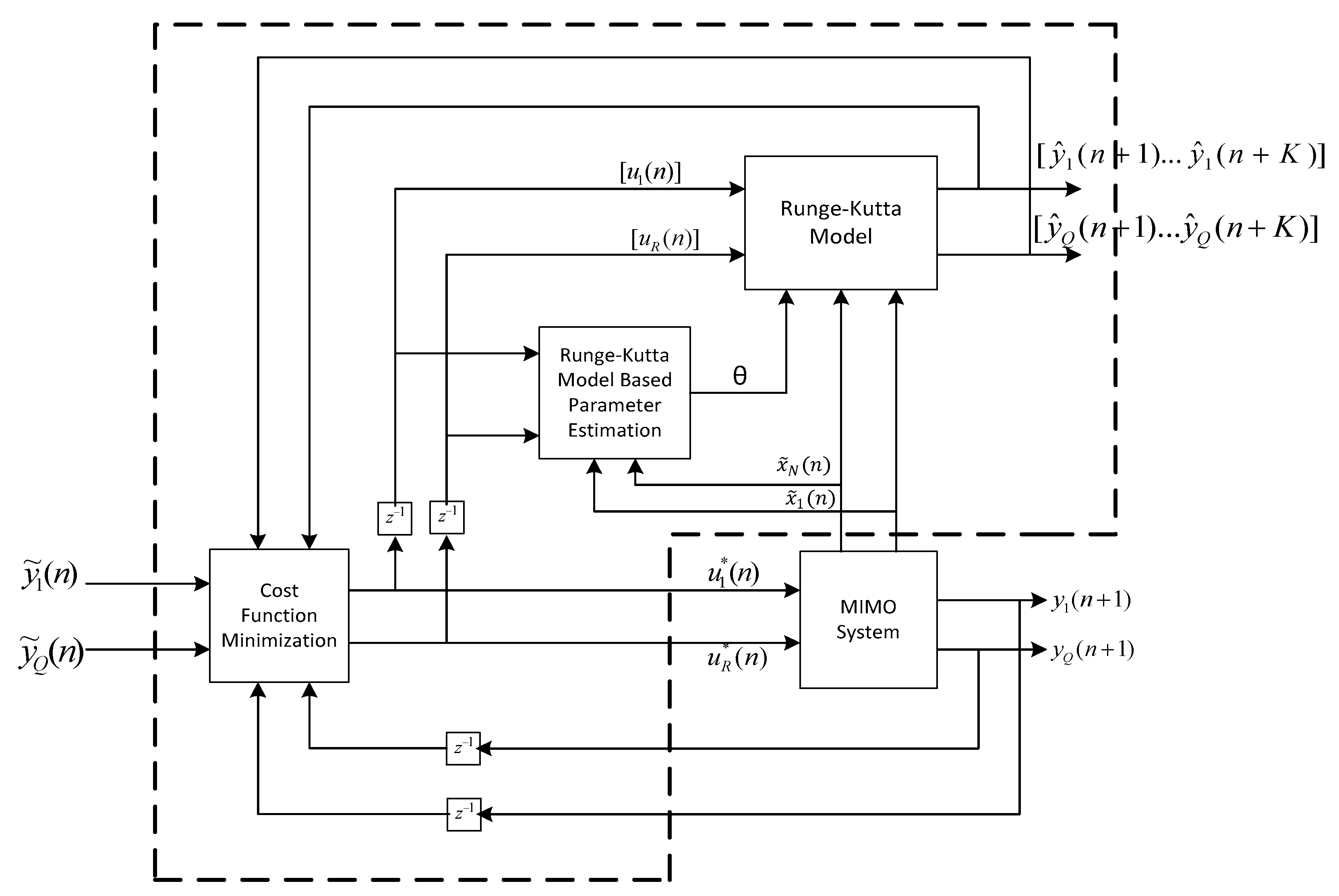
In this study, on the other hand, a novel control mechanism, RKMPC has been used for speed control of PMSM, where the current constraint $i_d^2+i_q^2<I_{max}^2$ and the voltage constraint $u_d^2+u_q^2<U_{max}^2$ of PMSM are combined and both current and voltage control of the system are controlled in a single loop. Also, i_d current is kept at zero for no attenuation in the field. Furthermore, the RKMPC method has been utilized for the adaptation of the speed of the motor under load variations via RKMPC-based online parameter estimation. RKMPC calculates future predictions and derivatives in each sampling period and minimizes the cost function. RKMPC method increases the computation burden while doing all these operations. Therefore, dSPACE DS1104 is used to make the calculations very fast in the PMSM speed control with RKMPC. The innovation of this study has been carried out via DS1104 to realize a PMSM speed control with nonlinear dynamics, the recently intended RKMPC method [18].

In traditional MPC, error minimization between reference and model prediction is essential and modulation is updated. In the RKMPC proposed in this study, modulation is not updated until it produces a control sign that will provide error optimization. Therefore, there may be a difference between the two when the controller is activated rather than the calculation load. In this respect, RKMPC is more stable, but it is an algorithm that is activated later for reference points that are far from reference. Although this seems to be a disadvantage, every control sign produced does not apply to the system and produces the optimum control sign that will provide more stable results. Instead of applying the control signal obtained in traditional MPC directly to the system, an optimization algorithm that will minimize the error is aimed. Thus, the most important motivation of this study is that the control sign obtained at the end of each calculation should be searched for the optimum control sign that will make the motor behavior more stable instead of driving the motor.

The paper is organized as follows: in Section 2, the mathematical model of PMSM is given. The RKMPC-based control and parameter estimation mechanism are introduced in Section 3. The details of the real-time implementation of the application are given in Section 4. Section 5 includes the experimental results, and the paper concludes with the conclusions and future work.

2. The Mathematical Model of PMSM

The first step in implementing the RKMPC strategy is to obtain the mathematical model of the system in the form of differential equations, which will later be used for future predictions and gradient calculations [18,19]. Under the assumption that the counter-EMF is sinusoidal and Eddy currents, hysteresis losses, and saturation are negligible, the nonlinear dynamical model of PMSM in (d-q) rotating reference framework is given by Equation (1) [20].

$$\begin{array}{c}\begin{array}{l}\frac{{\mathit{di}}_d}{\mathit{dt}}=-\frac{R}{L_d}{i}_d+\frac{L_q}{L_d}{p\omega }_r{i}_q+\frac{1}{L_d}{u}_d\\ \frac{{\mathit{di}}_q}{\mathit{dt}}=-\frac{R}{L_q}{i}_q-\frac{L_d}{L_q}{p\omega }_r{i}_d-\frac{\lambda p{\omega }_r}{L_q}+\frac{1}{L_q}{u}_q\\ \frac{{d\omega }_r}{\mathit{dt}}=\frac{p}{J}(\lambda i_q+(L_d-L_q)i_q{i}_d)-\frac{B}{J}{\omega }_r-\frac{T_L}{J}\end{array}\\ \begin{array}{c}x={\left[\begin{array}{ccc}{i}_d& i_q& {\omega }_r\end{array}\right]}^T\\ u={\left[\begin{array}{cc}{u}_d& u_q\end{array}\right]}^T\\ y={\left[\begin{array}{cc}{i}_d& {\omega }_r\end{array}\right]}^T\end{array}\end{array}$$

(1)

where $u_d$ and $u_q$ are d-axis and q-axis component of the armature voltage, respectively, $i_d$ and $i_q$ are d-axis and q-axis component of the armature current, respectively, $R$ is the per-phase stator resistance, $L_d$ and $L_q$ are d-axis and q-axis component of stator inductance, respectively, $\lambda$ is permanent magnet flux, ${\omega }_r$ is rotor speed, $T_L$ is load torque, $p$ is number of pole pairs, $J$ is moment of inertia, $B$ is coefficient of friction.

3. The Runge-Kutta Model Based Control Structure

3.1. The Runge- Kutta Model of a MIMO System

The mathematical model of PMSM given by Equation (1) can be rewritten in a more compact form as Equation (2).

$$\begin{array}{l}\dot{\mathbf{x}}(t)=\mathbf{f}(\mathbf{x}(t),\mathbf{u}(t),\theta )\\ \mathbf{y}(t)=\mathbf{g}(\mathbf{x}(t),\mathbf{u}(t))\end{array}$$

(2)

where

$$\begin{array}{c}{\dot{x}}_1(t)=f_1(x_1(t),\dots ,x_N(t),u_1(t),\dots ,u_R(t),\theta )\\ ⋮\\ {\dot{x}}_N(t)=f_N(x_1(t),\dots ,x_N(t),u_1(t),\dots ,u_R(t),\theta )\end{array}$$

(3)

$$\begin{array}{c}{y}_1(t)=g_1(x_1(t),\dots ,x_N(t),u_1(t),\dots ,u_R(t))\\ ⋮\\ y_Q(t)=g_Q(x_1(t),\dots ,x_N(t),u_1(t),\dots ,u_R(t))\end{array}$$

(4)

Equation (3) and Equation (4) are state equations and output equations, respectively. $R$ is the number of inputs, $N$ is the number of states and $Q$ is the number of outputs of the system, where $u_i(t)$ is the ith input, $x_i(t)$ is the ith state, and $y_i(t)$ is the ith output of the system at time t and $\theta$ is the parameter of the system. It is assumed that the functions $f_i(.)$s and $g_i(.)$s are known and continously differentiable. The next step in RKMPC is to obtain the discretized model of the system by using the standard fourth-order Runge-Kutta (RK) integration method. The discretized RK model of the system is given by Equation (5) and Equation (6).

$$\begin{array}{c}{\widehat{x}}_1(n+1)={\widehat{x}}_1(n)+\frac{k_{11}}{6}+\frac{k_{21}}{3}+\frac{k_{31}}{3}+\frac{k_{41}}{6}\\ ⋮\\ {\widehat{x}}_N(n+1)={\widehat{x}}_N(n)+\frac{k_{1N}}{6}+\frac{k_{2N}}{3}+\frac{k_{3N}}{3}+\frac{k_{4N}}{6}\end{array}$$

(5)

$$\begin{array}{c}{\widehat{y}}_1(n+1)=g_1({\widehat{x}}_1(n+1),\dots ,{\widehat{x}}_N(n+1),u_1(n),\dots ,u_R(n))\\ ⋮\\ {\widehat{y}}_Q(n+1)=g_Q({\widehat{x}}_1(n+1),\dots ,{\widehat{x}}_N(n+1),u_1(n),\dots ,u_R(n))\end{array}$$

(6)

where

$$\begin{array}{c}{k}_{11}=T_s{f}_1({\widehat{x}}_1(n),\dots ,{\widehat{x}}_N(n),u_1(n),\dots ,u_R(n))\hfill \\ ⋮\\ k_{1N}=T_s{f}_N({\widehat{x}}_1(n),\dots ,{\widehat{x}}_N(n),u_1(n),\dots ,u_R(n))\hfill \\ k_{21}=T_s{f}_1({\widehat{x}}_1(n)+\frac{k_{11}}{2},\dots ,{\widehat{x}}_N(n)+\frac{k_{1N}}{2},u_1(n),\dots ,u_R(n))\hfill \\ ⋮\\ k_{2N}=T_s{f}_N({\widehat{x}}_1(n)+\frac{k_{11}}{2},\dots ,{\widehat{x}}_N(n)+\frac{k_{1N}}{2},u_1(n),\dots ,u_R(n))\hfill \\ k_{31}=T_s{f}_1({\widehat{x}}_1(n)+\frac{k_{21}}{2},\dots ,{\widehat{x}}_N(n)+\frac{k_{2N}}{2},u_1(n),\dots ,u_R(n))\hfill \\ ⋮\\ k_{3N}=T_s{f}_N({\widehat{x}}_1(n)+\frac{k_{21}}{2},\dots ,{\widehat{x}}_N(n)+\frac{k_{2N}}{2},u_1(n),\dots ,u_R(n))\hfill \\ k_{41}=T_s{f}_1({\widehat{x}}_1(n)+k_{31},\dots ,{\widehat{x}}_N(n)+k_{3N},u_1(n),\dots ,u_R(n))\hfill \\ ⋮\\ k_{4N}=T_s{f}_N({\widehat{x}}_1(n)+k_{31},\dots ,{\widehat{x}}_N(n)+k_{3N},u_1(n),\dots ,u_R(n))\hfill \end{array}$$

(7)

The discretized RK model can put in a more compact form as seen in Equations (8) and (9).

$$\begin{array}{l}\widehat{\mathit{x}}(n+1)=\widehat{\mathbf{f}}(\widehat{\mathbf{x}}(n),\mathbf{u}(n))=\widehat{x}(n)+\frac{1}{6}{\mathbf{k}}_1+\frac{1}{3}{\mathbf{k}}_2+\frac{1}{3}{\mathbf{k}}_3+\frac{1}{6}{\mathbf{k}}_4\\ \widehat{\mathbf{y}}(n+1)=\mathbf{g}(\widehat{\mathbf{x}}(n+1),\mathbf{u}(n))\end{array}$$

(8)

$$\begin{array}{l}{\mathbf{k}}_1=\left[\begin{array}{c}{k}_{11}\\ ⋮\\ k_{N1}\end{array}\right]=\left[\begin{array}{c}{T}_s{f}_1(\widehat{\mathbf{x}},\mathbf{u})\\ ⋮\\ T_s{f}_N(\widehat{\mathbf{x}},\mathbf{u})\end{array}\right]=T_s\mathit{f}(\widehat{\mathbf{x}},\mathbf{u})\\ {\mathbf{k}}_2=\left[\begin{array}{c}{k}_{12}\\ ⋮\\ k_{N2}\end{array}\right]=\left[\begin{array}{c}{T}_s{f}_1(\widehat{\mathbf{x}}+0.5{\mathbf{k}}_1,\mathbf{u})\\ ⋮\\ T_s{f}_N(\widehat{\mathbf{x}}+0.5{\mathbf{k}}_1,\mathbf{u})\end{array}\right]=T_s\mathit{f}(\widehat{\mathbf{x}}+0.5{\mathbf{k}}_1,\mathbf{u})\\ {\mathbf{k}}_3=\left[\begin{array}{c}{k}_{13}\\ ⋮\\ k_{N3}\end{array}\right]=\left[\begin{array}{c}{T}_s{f}_1(\widehat{\mathbf{x}}+0.5{\mathbf{k}}_2,\mathbf{u})\\ ⋮\\ T_s{f}_N(\widehat{\mathbf{x}}+0.5{\mathbf{k}}_2,\mathbf{u})\end{array}\right]=T_s\mathit{f}(\widehat{\mathbf{x}}+0.5{\mathbf{k}}_2,\mathbf{u})\\ {\mathbf{k}}_4=\left[\begin{array}{c}{k}_{14}\\ ⋮\\ k_{N4}\end{array}\right]=\left[\begin{array}{c}{T}_s{f}_1(\widehat{\mathbf{x}}+{\mathbf{k}}_3,\mathbf{u})\\ ⋮\\ T_s{f}_N(\widehat{\mathbf{x}}+{\mathbf{k}}_3,\mathbf{u})\end{array}\right]=T_s\mathit{f}(\widehat{\mathbf{x}}+{\mathbf{k}}_3,\mathbf{u})\end{array}$$

(9)

3.2. The Runge-Kutta-Based Overall Control Structure

The overall structure of the RKMPC-based control and parameter estimation is given in Figure 1, where ${\tilde{y}}_i(.)$ is the ith reference signal specified by the user, ${\widehat{y}}_i(.)$ is the ith prediction signal of the RK model, $y_i(.)$ is the ith output signal of the system, and $K$ is the prediction horizon.

The structure of the RKMPC-based control and parameter estimation is composed of three blocks. The first one is the discretized RK model of the system, the second one is the cost function minimization (CFM) block, and the third one is the RK model-based parameter estimation block.

3.2.1. Runge-Kutta Model and Cost Function Minimization

In this structure the discretized RK model of the system plays a critical role since it is used for both future predictions and gradient calculations. In the MPC loop, a candidate vector of control actions is given by Equation (10).

$$\mathbf{u}(n)={[u_1(n),\dots ,u_R(n)]}^T$$

(10)

A candidate vector of control actions is obtained and before the system it is applied to the discretized RK model of the system in order to see what would happen if it was applied to the system repeatedly $K$ times. RK model produces up to $K$-step ahead the future predictions for each output of the system. In order to obtain an acceptable control vector to apply to the system, the CFM block tries to minimize the discrepancy between the reference signals and the future predictions of the RK model with respect to the control vector. More mathematically, the CFM block tries to minimize the cost function given in Equation (11).

$$F(\mathbf{u}(n))={\displaystyle \sum _{q=1}^Q\sum _{k=1}^K}{({\tilde{y}}_q(n+k)-{\tilde{y}}_q(n+k))}^2+{\displaystyle \sum _{r=1}^R}{\lambda }_r{(u_r(n)-u_r(n-1))}^2$$

(11)

where ${\lambda }_r$ is the rth penalty term. The resulting control signal is ${\mathbf{u}}^{*}(n)=\mathbf{u}(n)+\mathsf{\delta }\mathbf{u}(n)$ that provides a descend in the cost function, i.e., $F(\mathbf{u}(n)+\mathsf{\delta }\mathbf{u}(n))<F(\mathbf{u}(n))$, which then will be applied to the system to force its outputs towards the reference signals. Here the problem is how to obtain the sub-optimal correction term $\mathsf{\delta }\mathbf{u}(n)$. One remedy is to use the well-known optimization method, namely the Levenberg-Marquardt (LM), as given by Equation (12).

$$\mathsf{\delta }\mathbf{u}(n)=-{({\mathbf{J}}^T\mathbf{J}+\eta \mathbf{I})}^{-1}{\mathbf{J}}^T{\widehat{\mathbf{e}}}_c$$

(12)

where ${\widehat{\mathbf{e}}}_c$ is the vector of errors given by Equation (13)

$${\widehat{\mathbf{e}}}_c=\left[\begin{array}{c}\widehat{e}(n+1)\\ ⋮\\ \widehat{e}(n+K)\\ ⋮\\ \widehat{e}(n+KQ)\\ \sqrt{{\lambda }_1}\Delta u_1(n)\\ ⋮\\ \sqrt{{\lambda }_R}\Delta u_R(n)\end{array}\right]=\left[\begin{array}{c}{\tilde{y}}_1(n+1)-{\widehat{y}}_1(n+1)\\ ⋮\\ {\tilde{y}}_1(n+K)-{\widehat{y}}_1(n+K)\\ ⋮\\ {\tilde{y}}_Q(n+K)-{\widehat{y}}_Q(n+K)\\ \sqrt{{\lambda }_1}\left[u_1(n)-u_1(n-1)\right]\\ ⋮\\ \sqrt{{\lambda }_R}\left[u_R(n)-u_R(n-1)\right]\end{array}\right]$$

(13)

and $\eta$ is a parameter that provides a compromise between the steepest-descent and Gauss-Newton directions and $\mathbf{J}$ is the Jacobian matrix given by Equation (14).

$$\mathbf{J}=-\left[\begin{array}{c}\begin{array}{cccc}\frac{\partial {\widehat{y}}_1(n+1)}{\partial u_1(n)}& \frac{\partial {\widehat{y}}_1(n+1)}{\partial u_2(n)}& \cdots & \frac{\partial {\widehat{y}}_1(n+1)}{\partial u_R(n)}\\ ⋮& ⋮& \ddots & ⋮\\ \frac{\partial {\widehat{y}}_1(n+K)}{\partial u_1(n)}& \frac{\partial {\widehat{y}}_1(n+K)}{\partial u_2(n)}& \cdots & \frac{\partial {\widehat{y}}_1(n+K)}{\partial u_1(n)}\\ ⋮& ⋮& \ddots & ⋮\end{array}\\ \begin{array}{cccc}\frac{\partial {\widehat{y}}_Q(n+K)}{\partial u_1(n)}& \frac{\partial {\widehat{y}}_Q(n+K)}{\partial u_2(n)}& \cdots & \frac{\partial {\widehat{y}}_Q(n+K)}{\partial u_R(n)}\\ \sqrt{{{\displaystyle \lambda }}_1}& \sqrt{{{\displaystyle \lambda }}_1}& \cdots & \sqrt{{{\displaystyle \lambda }}_1}\\ ⋮& ⋮& \ddots & ⋮\\ \sqrt{{{\displaystyle \lambda }}_R}& \sqrt{{{\displaystyle \lambda }}_R}& \cdots & \sqrt{{{\displaystyle \lambda }}_R}\end{array}\end{array}\right]$$

(14)

The ithjth term $\frac{\partial {\widehat{y}}_i(n+K)}{\partial u_j(n)}$ of the Jacobian matrix is obtained by Equation (15)–(19).

$$\frac{\partial \widehat{\mathbf{y}}(n+k)}{\partial \mathbf{u}(n)}={[\frac{{\partial }^T\mathbf{g}}{\partial \mathbf{x}}\frac{\partial \widehat{\mathbf{x}}(n+k)}{\partial \mathbf{u}(n)}]}_{\mathbf{x}=\widehat{\mathbf{x}}(n+k)}$$

(15)

$$\frac{\partial \widehat{\mathbf{x}}(n+h)}{\partial \mathbf{u}(n)}={[\frac{\partial \widehat{\mathbf{f}}}{\partial \mathbf{x}}\frac{\partial \widehat{\mathbf{x}}(n+k-1)}{\partial \mathbf{u}(n)}+\frac{\partial \widehat{\mathbf{f}}}{\partial \mathbf{u}}]}_{\underset{\mathit{u}=\mathit{u}(n)}{\mathbf{x}=\widehat{\mathbf{x}}(n+k-1)}}$$

(16)

$$\begin{array}{l}\frac{\partial \widehat{\mathbf{f}}}{\partial \mathbf{x}}=\frac{\partial {\mathbf{x}}_{\mathbf{i}}(n)}{\partial \mathbf{x}(n)}+[\frac{1}{6}\frac{\partial {\mathbf{k}}_{\mathbf{1}}}{\partial \mathbf{x}}+\frac{1}{3}\frac{\partial {\mathbf{k}}_{\mathbf{2}}}{\partial \mathbf{x}}+\frac{1}{3}\frac{\partial {\mathbf{k}}_{\mathbf{3}}}{\partial \mathbf{x}}+\frac{1}{6}\frac{\partial {\mathbf{k}}_{\mathbf{4}}}{\partial \mathbf{x}}]\\ \frac{\partial \widehat{\mathbf{f}}}{\partial \mathbf{u}(n)}=[\frac{1}{6}\frac{\partial {\mathbf{k}}_{\mathbf{1}}}{\partial \mathbf{u}(n)}+\frac{1}{3}\frac{\partial {\mathbf{k}}_{\mathbf{2}}}{\partial \mathbf{u}(n)}+\frac{1}{3}\frac{\partial {\mathbf{k}}_{\mathbf{3}}}{\partial \mathbf{u}(n)}+\frac{1}{6}\frac{\partial {\mathbf{k}}_{\mathbf{4}}}{\partial \mathbf{u}(n)}]\end{array}$$

(17)

$$\begin{array}{l}\frac{\partial {\mathbf{k}}_{\mathbf{1}}}{\partial \mathbf{x}}=T_s{[\frac{\partial \mathbf{f}}{\partial \mathbf{x}}]}_{\underset{u=u(n)}{x=\widehat{x}(n)}}\\ \frac{\partial {\mathbf{k}}_{\mathbf{2}}}{\partial \mathbf{x}}=T_s{[\frac{\partial \mathbf{f}}{\partial \mathbf{x}}(\mathbf{I}+0.5\frac{\partial {\mathbf{k}}_{\mathbf{1}}}{\partial \mathbf{x}})]}_{\underset{\mathbf{u}=\mathbf{u}(n)}{\mathbf{x}=\widehat{\mathbf{x}}(n)+0.5{\mathbf{k}}_{\mathbf{1}}}}\\ \frac{\partial {\mathbf{k}}_{\mathbf{3}}}{\partial \mathbf{x}}=T_s{[\frac{\partial \mathbf{f}}{\partial \mathbf{x}}(\mathbf{I}+0.5\frac{\partial {\mathbf{k}}_{\mathbf{2}}}{\partial \mathbf{x}})]}_{\underset{\mathbf{u}=\mathbf{u}(n)}{\mathbf{x}=\widehat{\mathbf{x}}(n)+0.5{\mathbf{k}}_{\mathbf{2}}}}\\ \frac{\partial {\mathbf{k}}_{\mathbf{4}}}{\partial \mathbf{x}}=T_s{[\frac{\partial \mathbf{f}}{\partial \mathbf{x}}(\mathbf{I}+\frac{\partial {\mathbf{k}}_{\mathbf{3}}}{\partial \mathbf{x}})]}_{\underset{\mathbf{u}=\mathbf{u}(n)}{\mathbf{x}=\widehat{\mathbf{x}}(n)+{\mathbf{k}}_{\mathbf{3}}}}\end{array}$$

(18)

$$\begin{array}{c}\begin{array}{l}\frac{\partial {\mathbf{k}}_{\mathbf{1}}}{\partial \mathbf{u}(n)}=T_s{[\frac{\partial \mathbf{f}}{\partial \mathbf{u}(n)}]}_{\underset{\mathbf{u}=\mathbf{u}(n)}{\mathbf{x}=\widehat{\mathbf{x}}(n)}}\\ \frac{\partial {\mathbf{k}}_{\mathbf{2}}}{\partial \mathbf{u}(n)}=T_s{[\left(0.5\frac{\partial \mathbf{f}}{\partial \mathbf{x}}\frac{\partial {\mathbf{k}}_{\mathbf{1}}}{\partial \mathbf{u}(n)}\right)+\frac{\partial \mathbf{f}}{\partial \mathbf{u}(n)}]}_{\underset{u=\mathbf{u}(n)}{\mathbf{x}=\widehat{\mathbf{x}}(n)+0.5{\mathbf{k}}_{\mathbf{1}}}}\\ \frac{\partial {\mathbf{k}}_{\mathbf{3}}}{\partial \mathbf{u}(n)}=T_s{[\left(0.5\frac{\partial \mathbf{f}}{\partial \mathbf{x}}\frac{\partial {\mathbf{k}}_{\mathbf{2}}}{\partial \mathbf{u}(n)}\right)+\frac{\partial \mathbf{f}}{\partial \mathbf{u}(n)}]}_{\underset{\mathbf{u}=\mathbf{u}(n)}{\mathbf{x}=\widehat{\mathbf{x}}(n)+0.5{\mathbf{k}}_{\mathbf{2}}}}\\ \frac{\partial {\mathbf{k}}_{\mathbf{4}}}{\partial \mathbf{u}(n)}=T_s{[\left(0.5\frac{\partial \mathbf{f}}{\partial \mathbf{x}}\frac{\partial {\mathbf{k}}_{\mathbf{3}}}{\partial \mathbf{u}(n)}\right)+\frac{\partial \mathbf{f}}{\partial \mathbf{u}(n)}]}_{\underset{\mathbf{u}=\mathbf{u}(n)}{\mathbf{x}=\widehat{\mathbf{x}}(n)+{\mathbf{k}}_{\mathbf{3}}}}\end{array}\\ \\ k=1,\dots ,K\end{array}$$

(19)

In order to keep the optimized control signal ${\mathbf{u}}^{*}(n)=\mathbf{u}(n)+\mathsf{\delta }\mathbf{u}(n)$ be within the allowable control limits a limiting coefficient $0<\mu <1$ is used as Equation (20).

$${\mathbf{u}}^{*}(n)=\mathbf{u}(n)+\mu \mathsf{\delta }\mathbf{u}(n)$$

(20)

where

$$\mu =\max (\frac{{\mathbf{u}}_{min}-\mathbf{u}}{\mathsf{\delta }\mathbf{u}(n)},\frac{{\mathbf{u}}_{max}-\mathbf{u}}{\mathsf{\delta }\mathbf{u}(n)})$$

(21)

3.2.2. The Runge-Kutta Model Based Online Parameter Estimation

The third block in the RKMPC structure is the parameter estimation block, where it is assumed that the measurements $\mathbf{u}(n)$, $\mathbf{x}(n)$ and $\mathbf{x}(n+1)$ are available. Thus, the unknown parameter $\theta$ of the system can be estimated as follows: Let $x_i(n+1)$ and ${\widehat{x}}_i(n+1)$ be the actual and predicted (by the RK model) values of the ith state at the time instant n + 1, respectively. Since the unknown parameter $\theta$ value is not available, there will be some errors between the actual and predicted values of the states, which are aggregated in a vector of errors as Equation (22).

$${\mathbf{e}}_{\theta }=\left[\begin{array}{c}{e}_1\\ e_2\\ \begin{array}{c}⋮\\ e_N\end{array}\end{array}\right]=\left[\begin{array}{c}{x}_1(n+1)-{\widehat{x}}_1(n+1)\\ x_2(n+1)-{\widehat{x}}_2(n+1)\\ \begin{array}{c}⋮\\ x_N(n+1)-{\widehat{x}}_N(n+1)\end{array}\end{array}\right]$$

(22)

This vector of errors can be back-propagated to the system parameter $\theta$ in order to obtain its correct value. This is accomplished as the update rule given by Equation (23).

$$\theta \leftarrow \theta -\frac{{\mathbf{J}}_{\theta }^T{\mathbf{e}}_{\theta }}{{\mathbf{J}}_{\theta }^T{\mathbf{J}}_{\theta }}$$

(23)

where ${\mathbf{J}}_{\theta }$ is the Jacobian matrix for parameter estimation given by Equation (24).

$${\mathbf{J}}_{\theta }=\left[\begin{array}{c}\frac{\partial e_1}{\partial \theta }\\ \frac{\partial e_2}{\partial \theta }\\ \begin{array}{c}⋮\\ \frac{\partial e_N}{\partial \theta }\end{array}\end{array}\right]=-\left[\begin{array}{c}\frac{\partial {\widehat{x}}_1(n+1)}{\partial \theta }\\ \frac{\partial {\widehat{x}}_2(n+1)}{\partial \theta }\\ \begin{array}{c}⋮\\ \frac{\partial {\widehat{x}}_N(n+1)}{\partial \theta }\end{array}\end{array}\right]$$

(24)

The partial derivatives $\frac{\partial {\widehat{x}}_i(n+1)}{\partial \theta }$ comprising the Jacobian matrix can be obtained by Equation (25) and Equation (26).

$$\frac{\partial {\widehat{x}}_i(n+1)}{\partial \theta }=\frac{\partial {\widehat{x}}_i(n)}{\partial \theta }+\frac{1}{6}\frac{\partial {\mathbf{k}}_{\mathbf{1}}}{\partial \theta }+\frac{1}{3}\frac{\partial {\mathbf{k}}_{\mathbf{2}}}{\partial \theta }+\frac{1}{3}\frac{\partial {\mathbf{k}}_{\mathbf{3}}}{\partial \theta }+\frac{1}{6}\frac{\partial {\mathbf{k}}_{\mathbf{4}}}{\partial \theta }$$

(25)

$$\begin{array}{l}\frac{\partial {\mathbf{k}}_{\mathbf{1}}}{\partial \theta }=T_s{[\frac{\partial \mathbf{f}}{\partial \theta }]}_{\begin{array}{c}\mathbf{x}(n)=\mathbf{x}(n)\\ \mathbf{u}=\mathbf{u}(n)\end{array}}\\ \frac{\partial {\mathbf{k}}_{\mathbf{2}}}{\partial \theta }=T_s{[(\frac{\partial \mathbf{f}}{\partial \theta }+0.5\frac{\partial \mathbf{f}}{\partial \mathbf{x}}\frac{\partial {\mathbf{k}}_{\mathbf{1}}}{\partial \theta })]}_{\begin{array}{c}\mathbf{x}(n)=\mathbf{x}(n)+0.5{\mathbf{k}}_{\mathbf{1}}\\ \mathbf{u}=\mathbf{u}(n)\end{array}}\\ \frac{\partial {\mathbf{k}}_{\mathbf{3}}}{\partial \theta }=T_s{[(\frac{\partial \mathbf{f}}{\partial \theta }+0.5\frac{\partial \mathbf{f}}{\partial \mathbf{x}}\frac{\partial {\mathbf{k}}_{\mathbf{2}}}{\partial \theta })]}_{\begin{array}{c}\mathbf{x}(n)=\mathbf{x}(n)+0.5{\mathbf{k}}_{\mathbf{2}}\\ \mathbf{u}=\mathbf{u}(n)\end{array}}\\ \frac{\partial {\mathbf{k}}_{\mathbf{4}}}{\partial \theta }=T_s{[(\frac{\partial \mathbf{f}}{\partial \theta }+0.5\frac{\partial \mathbf{f}}{\partial \mathbf{x}}\frac{\partial {\mathbf{k}}_{\mathbf{3}}}{\partial \theta })]}_{\begin{array}{c}\mathbf{x}(n)=\mathbf{x}(n)+{\mathbf{k}}_{\mathbf{3}}\\ \mathbf{u}=\mathbf{u}(n)\end{array}}\end{array}$$

(26)

$$\frac{\partial \widehat{\mathbf{f}}}{\partial \mathsf{\theta }}=\left[\frac{1}{6}\frac{\partial {\mathbf{k}}_{\mathbf{1}}}{\partial \theta }+\frac{1}{3}\frac{\partial {\mathbf{k}}_{\mathbf{2}}}{\partial \theta }+\frac{1}{3}\frac{\partial {\mathbf{k}}_{\mathbf{3}}}{\partial \theta }+\frac{1}{6}\frac{\partial {\mathbf{k}}_{\mathbf{4}}}{\partial \theta }\right]$$

(27)

3.3. Application of RKMPC to PMSM

Figure 2 shows the control block diagram of the RKMPC method. As can be seen from the Figure 2, three A/D converters are used, two of them are to measure the phase currents and one is to measure the DC voltage. The phase currents read from the A/D converters are first mapped by the Clark transform $(a,b,c\to \alpha ,\beta )$ and then Park transform ($\alpha ,\beta \to d,q)$, and then they are formed as the state vector together with the speed signal from the encoder, which will later be used in the RKMPC algorithm.

Additionally, the signal conveying the position information of the rotor received from the encoder is used in Park and Inverse Park transforms. The position and the speed of the rotor are measured by using an incremental encoder (2500 ppr). Obtained PWM signals are transferred to the IGBT inverter via IGBT driver circuit. The inputs $u_d$ and $u_q$ are mapped by inverse Park transform $d,q\to \alpha ,\beta$, then they are sent to the SVPWM block to produce PWM signals. The RKMPC algorithm produces the proper outputs ($i_d$ and ${\omega }_r$).

Application of RKMPC Algorithm

The implementation of the RKMPC algorithm is shown in Figure 3. In the algorithm, at each sampling period, the x(n) state values, the u(n − 1) final control signal, and the $\tilde{y}(n)$ reference vector are obtained to perform the calculation of the RKMPC algorithm.

The algorithm calculates K-step predictions and derivatives simultaneously using the RKModel of the proposed model. $\mathsf{\delta }u(n)$ is obtained by simple division of the terms Hessian and Gradient from Equation (12). Afterwards, an optimized control signal is obtained by updating ${\mathbf{u}}^{*}(n)=\mathbf{u}(n)+\mathsf{\delta }\mathbf{u}(n)$.

In addition, errors are obtained by taking the difference between real and predicted states in changing system parameters. These parameters are updated by applying Equation (23).

4. Real-Time Application

In order to test the RKMPC mechanism on the PMSM system, an experimental setup has been established, which can be seen in Figure 4. The setup is composed of a dSPACE DS1104 ACE Kit, a PMSM, a speed sensor, and a IGBT inverter. Moreover, another PMSM generator is coupled as the load.

The dSPACE 1104 board is a powerful tool for rapid control applications, which consists of a master processor PowerPC603 with speed of 250 MHz, 64-bit floating-point processor, and a slave-DSP subsystem based on the Texas Instruments TMS320F240 DSP microcontroller 20 MHz. The RKMPC algorithm has been implemented on the main processor and the slave unit has been dedicated to the SVPWM signals generation and to the management of the digital I/O signals.

As can be seen in Figure 5, a real-time overall MATLAB/Simulink block is developed to use the dSPACE1104 board in the control loop, where voltages and currents are obtained in the measurement block, while speed and position information are obtained in the speed block. The RKMPC algorithm is implemented in the MPC block. PWM signals are obtained in the SVPWM block at the 5 kHz constant sampling frequency.

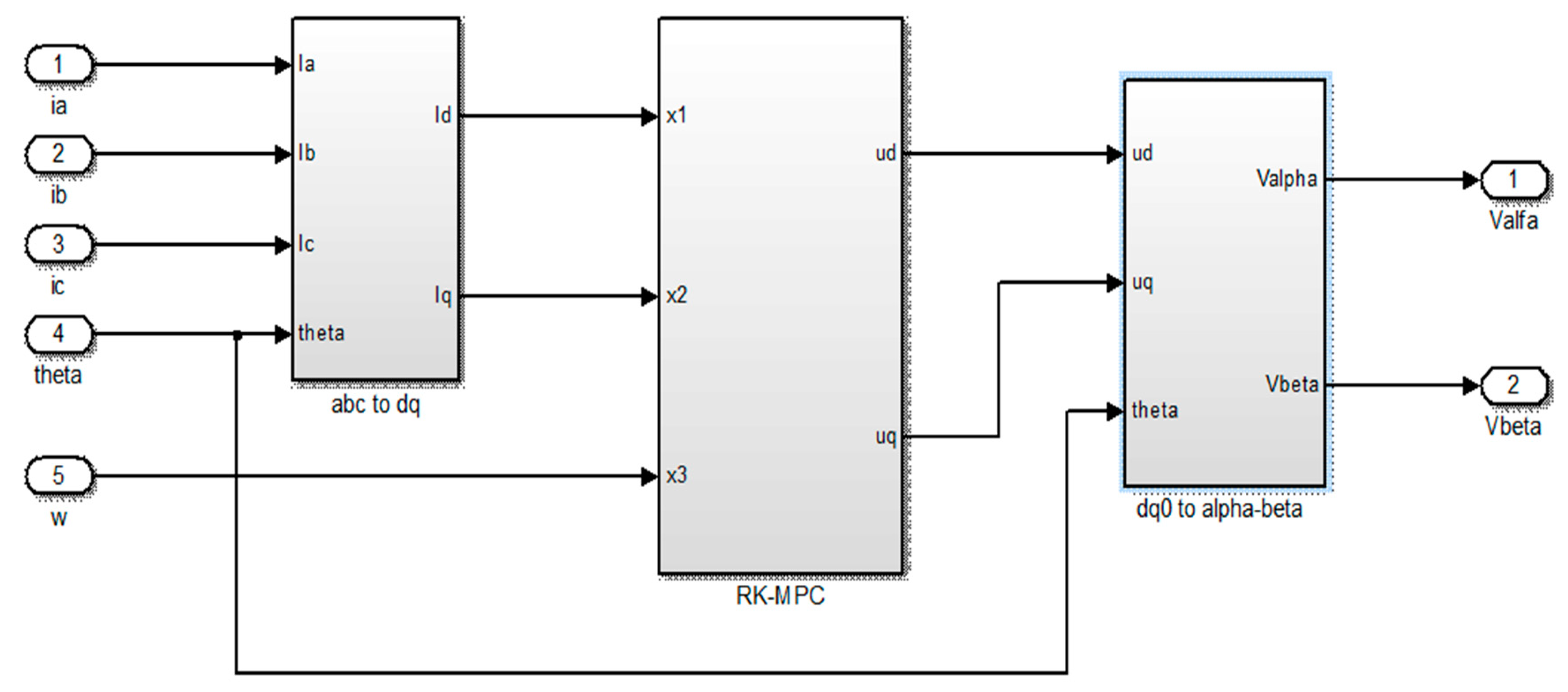
Model predictive control block is shown in Figure 6. In this block, Clark transform (a, b, c → α, β) and then Park transform (α, β → d, q) are also made. All algorithms are implemented in the RKMPC block.

The parameter values of the used PMSM driver are tabulated in

Table 1. The parameters of the Permanent magnet synchronous motor (PMSM).

Description	Value	Unit
Rated speed	3000	r/min
Rated current	2.8	A
Rated torque	1.27	Nm
Stator resistance	2.5	Ω
d-axes inductance	7	mH
q-axes inductance	7	mH
Pole pair number	4
Motor inertia	3.13 × 10−5	kgm2

.

5. Experimental Results and Comparisons

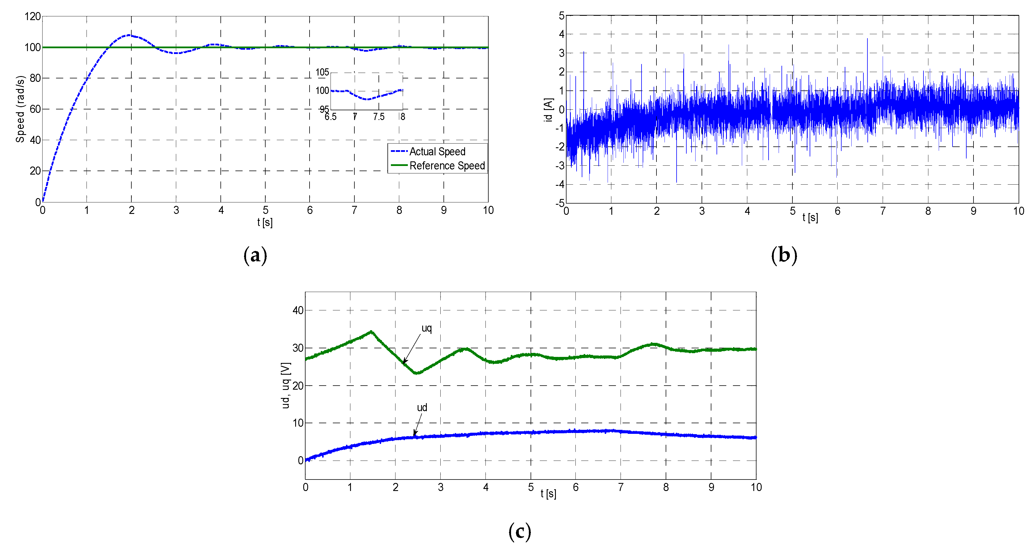
In order show the efficiency of the RKMPC method, it has been tested in different operating conditions. In the first case, PMSM has no load, while in the second case PMSM is loaded. Figure 7 shows the experimental results for RKMPC, where $i_d$, $i_q,$ $u_d$, and $u_q$ of PMSM are obtained under the nominal conditions for 100 rad/s reference speed without load, respectively. As can be seen from Figure 7, outputs of the system rise to the desired values very fast and then follow the reference trajectories accurately with zero steady state errors. Furthermore, RKMPC has been compared to a conventional PI controller, the parameters of which are tuned by trial-and-error. Figure 8 shows the experimental results for PI, where $i_d$,$i_q,$ $u_d,$ and $u_q$ of PMSM are obtained under the nominal conditions for 100 rad/s reference speed without load, respectively.

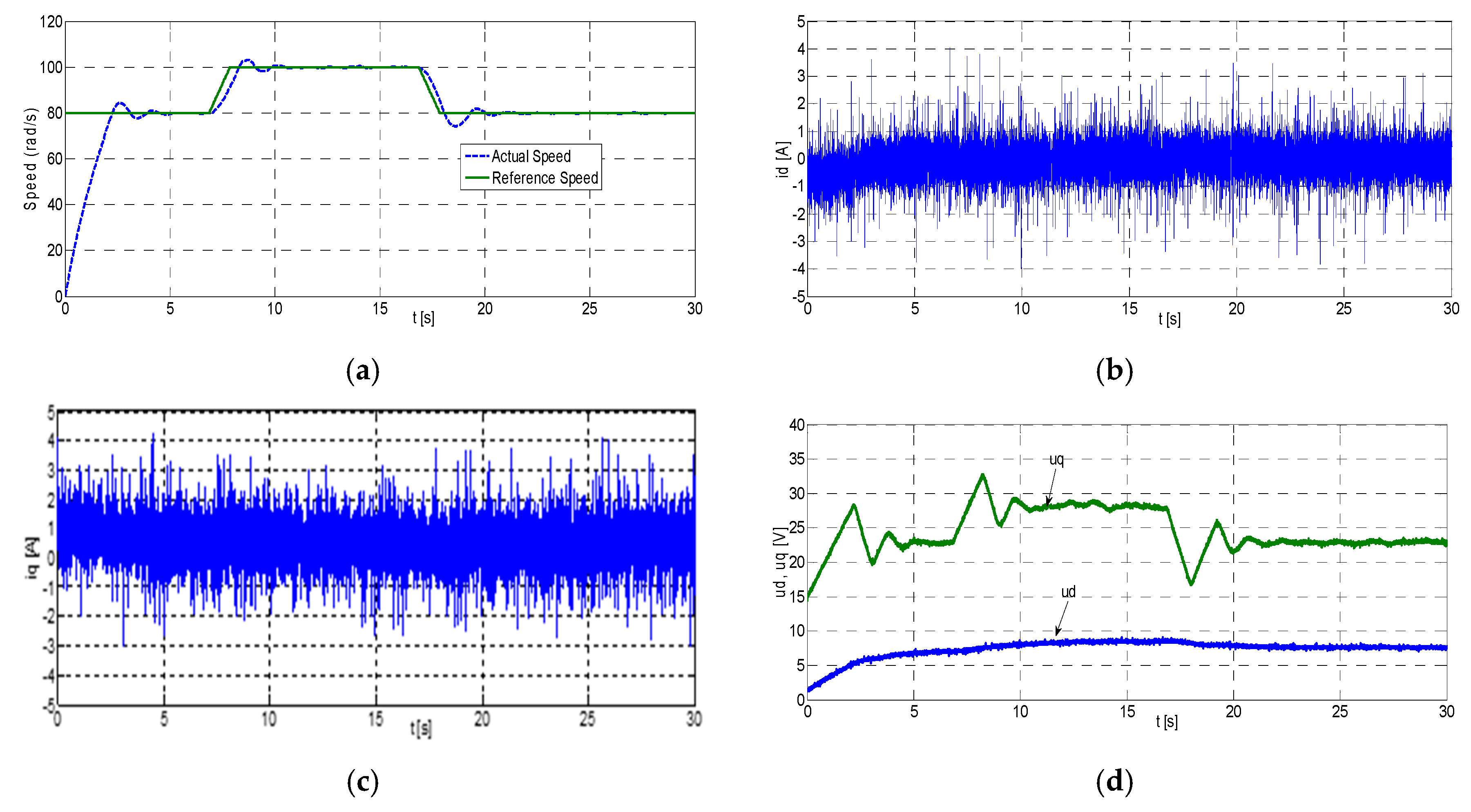
Afterwards, tests are repeated under the same conditions except for the reference signal is stepwise, i.e., it is initially set to 80 rad/s and then set to 100 rad/s for 10 s, then set back to 80 rad/s. Figure 9 shows the experimental results for RKMPC, where $i_d$, $i_q,$ $u_d,$ and $u_q$ of PMSM are obtained under the nominal conditions for the stepwise reference speed without load, respectively. As can be seen from the figure, outputs of the system rise to the desired values very fast and then follow the reference trajectories accurately with zero steady state errors. Figure 10 shows the experimental results for PI, where $i_d$, $i_q,$ $u_d$, and $u_q$ of PMSM are obtained under the nominal conditions for the stepwise reference speed without load, respectively.

Afterwards, the tests are repeated for another operating condition where PMSM is loaded with a load of 70%. The results for the constant reference at 100 rad/s have been shown in Figure 11, where load is estimated by the RK model-based parameter estimation algorithm, thereby making RKMPC adaptive to the load changes. Figure 11 shows the experimental results for RKMPC, where $i_d$, $u_d$, and $u_q$ of PMSM are obtained under the nominal conditions for 100 rad/s reference speed with load, respectively. Figure 12 shows the experimental results for PI, where $i_d$, $u_d,$ and $u_q$ of PMSM are obtained under the nominal conditions for 100 rad/s reference speed with unknown load, respectively.

Finally, the experimental setup is started without load and the control mechanism forced PMSM to follow the constant speed reference at 100 rad/s. Afterwards, at a specific time at $t=2.8$ s, PMSM is loaded abruptly to 70% load to check the ability of RKMPC compensating the abrupt load disturbances. As can be seen from Figure 13, RKMPC adapts to the abrupt load changes so that the output of the system follows the reference trajectory very rapidly. Figure 14 shows the experimental results for PI, where $i_d$, $u_d,$ and $u_q$ of PMSM are obtained under the nominal conditions for abrupt load disturbance, respectively.

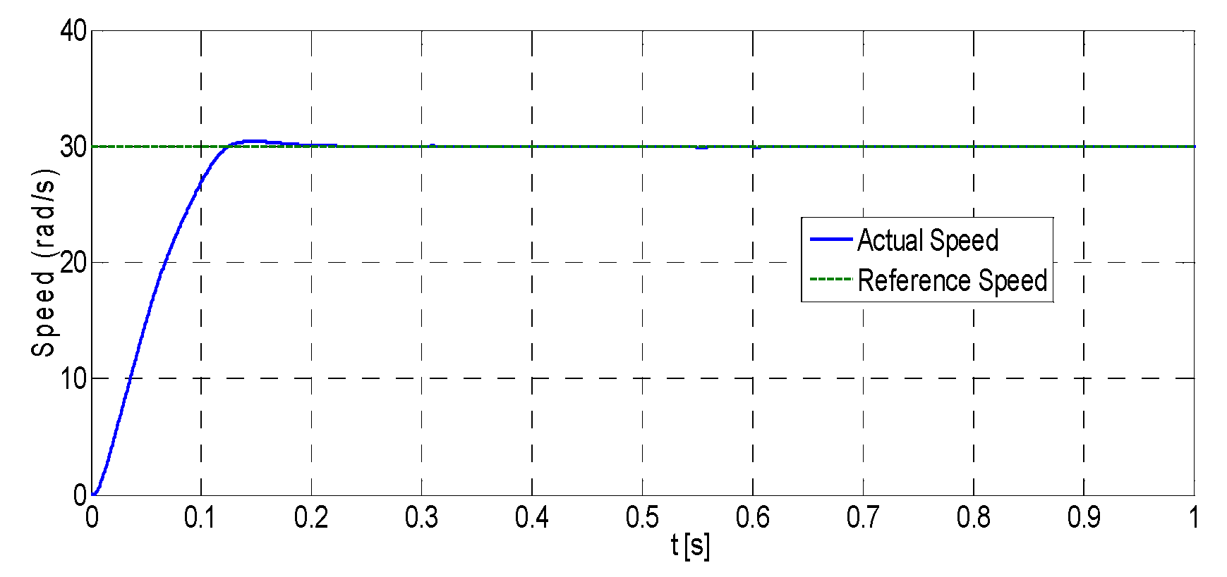
Moreover, RKMPC is evaluated at 30 rad/s and 200 rad/s reference speed values. Figure 15 shows the results for the 30 rad/s reference speed under the unloaded condition. Similarly, Figure 16 shows the results for the 200 rad/s reference speed under the unloaded condition.

In this study, under the same conditions, both RKMPC and traditional PI control methods were applied in loaded, unloaded, and abrupt load conditions. When both experimental results were compared, it was seen that RKMPC quickly reached the reference speed with almost zero excess. In conventional PI, it was seen that it reached the reference speed in a longer time and with a certain excess.

The same measuring circuits were used on the ds1104 board for the same parameters both in the use of the PI controller and in the application of the proposed RKMPC model. Therefore, measurement and evaluation units are the same in terms of measured variables. These noises are inevitable unless adaptive tuning of PI parameters is performed in real time.

6. Conclusions and Future Work

In this study, a recently proposed nonlinear control mechanism, which is referred to as the RKMPC method that combines the well-known numerical integration method Runge Kutta with the model predictive control framework, has been employed for control and load estimation of a commercial PMSM, where the constraints on the voltage and current of the system are taken into account. In the experiments, i_d current kept at zero for no attenuation in the field. It has been shown in the study that RKMPC mechanism can also estimate the load changes and unknown load disturbances to eliminate their undesired effects for a desirable control accuracy. RKMPC algorithm has been implemented on a dSPACE 1104 board. Then, its performance has been tested on a 0.4 kW PMSM motor experimentally for different conditions and compared to the conventional PI method. The tests have shown the efficiency of RKMPC for PMSMs, where RKMPC has provided satisfactory control performance even under load disturbances.

In future work, a new study using adaptive error method and adaptive hysteresis flux band needs to be done. In this way, for the big error values at the beginning, it will be ensured that the algorithm left in the loop to set the control condition to its optimum value will work with an increasingly adaptive error band. Thus, the proposed control algorithm will be enabled to control the system in closed loop from the beginning.

References

1. Chai, S.; Wang, L.; Rogers, E. Rogers Model predictive control of a permanent magnet synchronous motor with experimental validation. Control Eng. Pract. 2013, 21, 1584–1593. [Google Scholar] [CrossRef]
2. Du, R.H.; Wu, Y.F.; Chen, W.; Chen, Q. Adaptive Fuzzy Speed Control for Permanent Magnet Synchronous Motor Servo Systems. Electr. Power Components Syst. 2014, 42, 798–807. [Google Scholar] [CrossRef]
3. Li, S.; Liu, Z. Adaptive Speed Control for Permanent-Magnet Synchronous Motor System with Variations of Load Inertia. IEEE Trans. Ind. Electron. 2009, 56, 3050–3059. [Google Scholar]
4. Errouissi, R.; Ouhrouche, M.; Chen, W.-H. Robust nonlinear predictive control of a permanent magnet synchronous motor. In Proceedings of the IECON 2012—38th Annual Conference on IEEE Industrial Electronics Society, Montreal, QC, Canada, 25–28 October 2012; pp. 5057–5064. [Google Scholar]
5. Bolognani, S.; Peretti, L.; Zigliotto, M. Design and implementation of model predictive control for electrical motor drives. IEEE Trans. Ind. Electron. 2009, 56, 1925–1936. [Google Scholar] [CrossRef]
6. Rau, M.; Schröder, D. Model predictive control with nonlinear state space models. In Proceedings of the 7th International Workshop on Advanced Motion Control, Maribor, Slovenia, 3–5 July 2002; pp. 136–141. [Google Scholar]
7. Belda, K. Mathematical modelling and predictive control of permanent magnet synchronous motor drives. Trans. Electr. Eng. 2013, 2, 114–120. [Google Scholar]
8. Errouissi, R.; Ouhrouche, M.; Chen, W.-H.; Trzynadlowski, A.M. Robust cascaded nonlinear predictive control of a permanent magnet synchronous motor with antiwindup compensator. IEEE Trans. Ind. Electron. 2012, 59, 3078–3088. [Google Scholar] [CrossRef]
9. Fan, M.; Lin, H.; Lan, T. Model predictive direct torque control for SPMSM with load angle limitation. Prog. Electromagn. Res. B 2014, 58, 245–256. [Google Scholar] [CrossRef] [Green Version]
10. Mariethoz, S.; Domahidi, A.; Morari, M. Sensorless explicit model predictive control of permanent magnet synchronous motors. In Proceedings of the IEEE International Electric Machines & Drives Conference 2009 (IEMDC 2009), Miami, FL, USA, 3–6 May 2009; pp. 1250–1257. [Google Scholar]
11. Lin, C.-K.; Yu, J.-T.; Fu, L.-C.; Liu, T.-H.; Hsiao, C.-F. An improved predictive current control for interior permanent magnet synchronous motor drives based on current difference detection. In Proceedings of the 2012 IEEE/ASME International Conference on Advanced Intelligent Mechatronics, Kaohsiung, Taiwan, 11–14 July 2012; pp. 988–993. [Google Scholar]
12. Preindl, M.; Schaltz, E. Sensorless model predictive direct current control using novel second-order PLL observer for PMSM drive systems. IEEE Trans. Ind. Electron. 2011, 58, 4087–4095. [Google Scholar] [CrossRef]
13. Bobál, V.; Chalupa, P.; Kubalčík, M.; Dostál, P. Self-tuning predictive control of nonlinear servo-motor. J. Electr. Eng. 2010, 61, 365–372. [Google Scholar] [CrossRef] [Green Version]
14. Nguyen, H.T.; Jung, J.-W. Finite Control Set Model Predictive Control to Guarantee Stability and Robustness for Surface-Mounted PM Synchronous Motors. IEEE Trans. Ind. Electron. 2018, 65, 8510–8519. [Google Scholar] [CrossRef]
15. Formentini, A.; Trentin, A.; Marchesoni, M.; Zanchetta, P.; Wheeler, P. Speed Finite Control Set Model Predictive Control of a PMSM Fed by Matrix Converter. IEEE Trans. Ind. Electron. 2015, 62, 6786–6796. [Google Scholar] [CrossRef]
16. Kawai, H.; Zhang, Z.; Kennel, R. Finite Control Set-Model Predictive Speed Control with a Voltage Smoother. In Proceedings of the IECON—44th Annual Conference of the IEEE Industrial Electronics Society, Washington, DC, USA, 21–23 October 2018; pp. 528–533. [Google Scholar]
17. Yoo, H.-J.; Nguyen, T.-T.; Kim, H.-M. MPC with Constant Switching Frequency for Inverter-Based Distributed Generations in Microgrid Using Gradient Descent. Energies 2019, 12, 1156. [Google Scholar] [CrossRef] [Green Version]
18. Iplikci, S. Runge-Kutta model-based adaptive control mechanism for non-linear processes. Trans. Inst. Meas. Control 2012, 35, 166–180. [Google Scholar] [CrossRef]
19. Çetin, M.; Iplikci, S. A novel auto-tuning PID control mechanism for nonlinear systems. ISA Trans. 2015, 58, 292–308. [Google Scholar] [CrossRef] [PubMed]
20. Pillay, P.; Krishnan, R. Modeling of permanent magnet motor drives. IEEE Trans. Ind. Electron. 1998, 35, 537–541. [Google Scholar] [CrossRef] [Green Version]
Figure 1. Runge-Kutta-based control and parameter estimation structure.
Energies 13 01216 g001
Figure 2. Control block diagram of the Runge-Kutta model predictive control (RKMPC) method.
Energies 13 01216 g002
Figure 3. Application of RKMPC algorithm.
Energies 13 01216 g003
Figure 4. Experimental setup.
Energies 13 01216 g004
Figure 5. The real-time overall MATLAB/Simulink block.
Energies 13 01216 g005
Figure 6. Model predictive control block.
Energies 13 01216 g006
Figure 7. Experimental results for RKMPC for 100 rad/s reference speed without load. (a) Reference speed and measured speed of the motor; (b) i d current; (c) i q current; (d) u d and u q voltages.
Energies 13 01216 g007
Figure 8. Experimental results for PI for 100 rad/s reference speed without load. (a) Reference speed and measured speed of the motor; (b) i d current; (c) i q current; (d) u d and u q voltages.
Energies 13 01216 g008
Figure 9. Experimental results for RKMPC for stepwise reference speed without load. (a) Reference speed and measured speed of the motor; (b) i d current; (c) i q current; (d) u d and u q voltages.
Energies 13 01216 g009
Figure 10. Experimental results for PI for stepwise reference speed without load. (a) Reference speed and measured speed of the motor; (b) i d current; (c) i q current; (d) u d and u q voltages.
Energies 13 01216 g010
Figure 11. Experimental results for RKMPC for 100 rad/s reference speed with unknown load. (a) Reference speed and measured speed of the motor; (b) i d current; (c) u d and u q voltages.
Energies 13 01216 g011
Figure 12. Experimental results for PI for 100 rad/s reference speed with unknown load. (a) Reference speed and measured speed of the motor; (b) i d current; (c) u d and u q voltages.
Energies 13 01216 g012
Figure 13. Experimental results for RKMPC for abrupt load disturbance. (a) Reference speed and measured speed of the motor; (b) i d current; (c) u d and u q voltages.
Energies 13 01216 g013
Figure 14. Experimental results for PI for abrupt load disturbance. (a) Reference speed and measured speed of the motor; (b) i d current; (c) u d and u q voltages.
Energies 13 01216 g014
Figure 15. Experimental drive response to 30 rad/s reference speed under the unloaded condition with RKMPC.
Energies 13 01216 g015
Figure 16. Experimental drive response to 200 rad/s reference speed under the unloaded condition with RKMPC.
Energies 13 01216 g016