Thermal Assessment of Laminar Flow Liquid Cooling Blocks for LED Circuit Boards Used in Automotive Headlight Assemblies

Abstract

This research work presents a comparative thermal performance assessment of the laminar flow cooling blocks produced for automotive headlight assembly using a high power Light Emitting Diode (LED) chip. A three-dimensional numerical model with conjugate heat transfer in solid and fluid domains was used. Laminar flow was considered in the present analysis. The validation of the numerical model was realized by using the measured data from the test rig. It was observed that substantial temperature variations were occurred around the LED chip owing to volumetric heat generation. The cooling board with lower height performs better thermal performance but higher pressure drop for the same mass flow rates. The cooling board with the finned cover plate performs better thermal performance but results in an increased pressure drop for the same mass flow rates. Increasing the power of the LED results in higher temperature values for the same mass flow rates. The junction temperature is highly dependent on the mass flow rates and LED power. It can be controlled by means of the mass flow rate of the coolant fluid. New Nusselt number correlations are proposed for laminar flow mini-channel liquid cooling block applications.

1. Introduction

Recent trends in lighting systems focus on low energy consumption, higher light quality and reliability, long operation life, variable color, and low environmental impact [1,2]. Since light-emitting diode (LED) lighting presents superior performance and application flexibility over traditional incandescent lighting systems, it has found a wide range of applications in the automotive industry [3,4]. In addition to low energy consumption and high lighting performance, other reasons for preferring the LED lighting systems are shorter response times and longer service life (up to 100,000 hours) than traditional ones [5,6]. The regular LED rating current is about 20 mA, LEDs with a rating current higher than 20 mA can be classified as high power LEDs. Currently, the power of the high power LEDs can be in the range of 1 W to 21 W. High power LEDs provide higher quality light beam and brightness as well as to be the best solid-state light source enabling to realize the innovative ideas about lighting applications. Previously, LEDs commonly appeared on the automobile exteriors such as signal indicators, tail, reverse, and brake lights. Since the progress and recent innovations in LED lighting technology have shown a significant improvement in recent years, high power LEDs have appeared as headlight applications in automobiles [7,8]. However, LED lighting systems have a severe thermal problem like other high technology electronic devices. About 70–80% of the supplied electric power to the LED is converted into heat at a quite localized area as a hot spot during operation. Considering a high power LED with 1 W rating power have a 1 mm² heat transfer area on the chip die, the corresponding heat flux is 100 W/cm². This localized heat production results in a substantial increase in the junction temperature which has a significant effect on the lighting and thermal performance of the LED system while also shortening the expected operating life of LEDs. Because of this, thermal management of LED systems with active cooling to control the LED junction temperature under the value defined by LED manufacturers has been a significant scientific interest as well as a technological improvement [9,10]. Therefore, further researches are needed on the active cooling of LED systems for reliable operation and long service life. One of the widely used cooling methods is the extended surfaces or finned type heat sinks, which have lower operational cost and easy application. Many research articles dealing with extended surface type heat sinks for cooling of LEDs were published in the current literature [11]. Since the primary heat transfer mechanism between the finned heat sink and the environment air is the natural or forced convection, it has some drawbacks such as relatively significant temperature difference between the solid surface and the air, longer response time for cooling effect and relatively large volume for the required heat transfer rates [12]. Nevertheless, extended surfaces heat sinks are usually insufficient to provide enough cooling rates for the high-power LEDs. Other less common thermal management methods such as microjet cold plates [13,14], thermoelectric refrigeration [15], liquid metal cooling of cold plates [16], porous media micro cooling blocks [17], heat pipe applications [18], ferrofluid coolant [19], electric field control [20], and monolayer applications [21] have been published in the current literature. Liquid cooling blocks present an effective cooling alternative for the LED’s cooling as well as other cooling applications on electronic devices, batteries, etc. [12]. Since the specific heat and heat transfer coefficient is quite higher than air, it is more appropriate for the cooling based thermal management applications.

As automotive manufacturers seek reduced fuel consumption and lower emissions, decreasing the electrical load on an automobile has become more important. LEDs have been used widely in dashboard lightings and signal lightings in the automotive industry. Most new automobiles come with LED daytime running lights, but full LED headlights are not industry standard yet. The progress in automotive lighting systems with high illumination quality as well as reliability is necessary for driving safety and comfort. However, automotive headlight assembles have enclosed volumes, and there are very limited spaces in which LED PCBs located. Moreover, they are installing near the engine and the internal temperature is considerably higher than ambient in those regions. On the other hand, the light output quality and lighting performance strongly depend on the junction temperature and driven current. Therefore, active cooling systems with efficient energy management become very crucial for automotive headlight systems.

Although there are several studies considering LED cooling and thermal management, there are a few studies, such as the references [7,8,12], considering the high power LEDs for automotive headlight applications. Among these studies, there is a very rare study considering the liquid cooling applications in the automotive LED lighting systems. The purpose of this study is, firstly, to perform a detailed comparative thermal and hydraulic performance evaluation of the laminar flow cooling blocks used automotive headlight assembly combined with high power LED chips, and secondly, to provide enough cooling to control the junction temperature of the LED under the maximum allowable value defined by the manufacturer. Numerical analysis are performed using three dimensional simulation model with real dimensions. Two types of cover as finned and plane plate are employed in the numerical analysis. Besides the numerical study, theoretical and experimental investigations are also performed to validate the numerical analysis. With these respects, the novelty and the main contributions to the current literature of the present study may be stated as follows:

A PCB with high power LEDs is manufactured according to the real applications on the automotive headlight system. Meanwhile, the cooling blocks with appropriate size and dimensions are manufactured to be coupled with the produced PCB and they are employed in the measurements presented in this study.

A realistic three-dimensional numerical model for the cooling block incorporating the PCB and its real dimensions and components is generated. The model is validated with the experimental measurements and the theoretical approaches in the literature. Then, the detailed numerical analysis is performed for the flow and conjugate heat transfer in solid and fluid domains. The obtained results are evaluated and generalized with the non-dimensional parameters as Reynolds number (Re) and Nusselt number (Nu). New Nu number correlations are proposed to use as a reference for further studies.

2. Materials and Methods

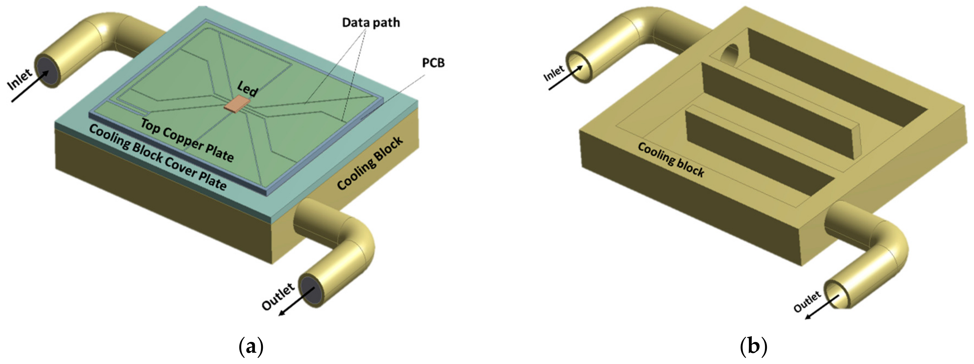
2.1. LED System Design and Experimental Set-up

The LED system used in this study includes two different regions. The first one consists of an electronic printed circuit board (PCB) between the top and bottom copper plates, and the second one is a cooling block that had cooling channels immersed in a fluid zone demonstrated in Figure 1a,b, respectively. The dimensions of the LED PCB are 60 mm × 51 mm × 1.62 mm. It has two 35 µm thick copper plates on both sides. The material of the PCB is FR4. The LED chip was placed on the top copper of the PCB. Two types of cooling block cover were used as a plane plate and a finned plate. Dimensions of the cooling block and the cover are shown in Figure 2a,b, respectively.

The height of the aluminum block was selected as 7 mm and 9 mm in order to get the effect of channel height on the thermal performance of the liquid cooling block. The cooling fluid flows through a channel in the block so that to cool down the LED PCB located on the cover plate. During the tests, temperatures were read and recorded at six different points on the upper surface of the PCB, as appear in Figure 3. Measurements were realized by the use of K-type thermocouples. Positions of the thermocouples were selected to obtain the variation of temperature over the PCB upper surface. After steady-state conditions reached, measurements were performed and recorded at every second for the 15 minutes’ time interval. Measurements were repeated several times with the same conditions. The data obtained from the measurements were used to validate the computed model results.

The schematic representation of the test rig is appearing in Figure 4a. The cooling water is stored in a one-liter water tank (1), the temperature of the fluid in the tank is measured by the J-type bayonet thermocouple. The cooling fluid continuously circulates in the system through a pump (2). The power of the coolant pump can be adjusted to circulate the fluid at different mass flow rates, and it is appropriate to operate on the cooling fluid temperature range of 5 to 60 °C. A turbine-type flow meter (3) is employed to observe the fluid flow rate. The cooling fluid flows through the block (4) to cool the LED PCB. The heated fluid is cool down through the heat sink unit (5). Then it flows to the storage tank. Fluid circulation system components are connected to each other utilizing flexible PVC pipes, which have an 8 mm diameter. An electronic control unit is mounted into the test rig to control and drive the components in the system. Figure 4b shows a photograph of the test setup. All the measured data is recorded in a data logger. Measurement devices used for the temperature and flow rate measurements were listed in

Table 1. The measurement devices used in the experimental study.

Type	Measuring Range	Uncertainty
K-type thermocouple	−40 °C/400 °C	±0.75%
Flowmeter	0–30 L/min	±1%

. The uncertainties of the measured data were calculated by the use of the method described in the study of Moffat [22]. The total error in the measured data was calculated in the range of ±3.5%. Properties of the LED chip employed in the present work are given in

Table 2. Characteristics of the LED chip used in this study.

Parameter	Symbol	Values	Unit
Operating Temperature	Top	−40–125	°C
Maximum Junction Temperature for short time app.)	Tj,max	175	°C
Maximum Junction Temperature (for long time app.)	Tj,max	150	°C
Current	IF	50–1200	mA
Voltage	VF	10.90–14.90	V
Luminous Flux (IF = 1000 mA)	ΦV	1120–1250	lm
Radiating Surface	Acolor	4.4	mm2
Junction Point Real Thermal Resistance	Rth,Jp	1.0	°C/W

.

2.2. Numerical Modeling of the Cooling Block with LED PCB

The CAD model of the cooling block with LED PCB is given in Figure 1 and Figure 2. The fluid domain in the model was created by using the CAD model of the cooling block system. To obtain the distributions of velocity, pressure, and temperature in the fluid part of the solution domain, continuity, momentum, and energy equations were solved by using the finite volume method. Meanwhile, only the energy equation was solved in the solid parts of the solution domain. Therefore, a conjugate analysis for the solution domain was realized by the use of Ansys Fluent CFD code. Details of the governing equations and the software can be found in the reference [23]. Numerical computations were conducted under steady-state conditions with constant properties. Laminar flow conditions were assumed in the block, and the SIMPLE method was employed for pressure–velocity coupling. Applying the conservation laws for mass, momentum, and energy, governing equations can be written as given in Equations (1) to (4):

Continuity equation for the fluid domain:

$$\nabla \left(\rho \overrightarrow{V}\right)=0$$

(1)

Momentum equation for fluid domain:

$$\overrightarrow{V}\cdot \nabla \left(\rho \overrightarrow{V}\right)=-\nabla p+\nabla \cdot \left(\mu \nabla \overrightarrow{V}\right)$$

(2)

The energy equation for the fluid domain:

$$\overrightarrow{V}\cdot \nabla \left(\rho c_{p}T\right)=\nabla \cdot \left(k_f\nabla T\right)$$

(3)

The energy equation for the solid domain:

$$\nabla \cdot \left(k_s\nabla T\right)+S=0$$

(4)

where $\overrightarrow{V}$ (m/s) is the velocity vector; p (Pa) is the pressure; c_p (J/kg·K) is the specific heat of fluid at the constant pressure; µ (Pa.s) is the fluid dynamic viscosity; ρ (kg·m⁻³) is the fluid density; T (°C) is the temperature; k_f and k_s (Wm⁻¹·K⁻¹) represent the heat transfer coefficients at the fluid domain and the solid domain, respectively. In the energy equation for the solid domain, S is the source term includes volumetric heat generation for the LED chip part and this term can be neglected for the other solid zones.

The mesh structure of the numerical model is shown in Figure 5. Due to the importance of the stability and accuracy in the numerical computations, Cartesian mesh structure which is consists of mostly hexahedral elements is employed in the model. Four million mesh elements in the whole fluid and solid solution domain is used. Considering the temperature variations near the LED chip, we used high mesh intensity surrounding the LED chip which had a size of 10 × 15 mm. Since the mesh structure significantly affects the accuracy of the results and the solution time, a grid dependence test was performed. It is found that four million elements in total are enough for the grid-independent analysis.

Table 3. Boundary conditions and materials used in the numerical simulation.

Surfaces or Domains	Boundary Conditions
Supply temperature of the coolant	Constant temperature value of 23.45 °C
Outlet surface of the cooling block	Gauge pressure equals to 0 Pa
Mass flow rate of coolant	Between 0.0005 to 0.01 kg/s
LED chip	Volumetric heat generation rate
Outer surfaces of solid domains	Convection and radiation mixed boundary conditions
Material type	Solid domains
LED chip	Chip material
Top and bottom copper plates	Copper
Printed Circuit Board	Glass-reinforced epoxy laminate material (FR4)
Cover plate	Aluminum
Cooling Block	Aluminum

shows the boundary conditions and the materials used in the model.

The normalized residuals (NR) are used as convergence criteria. It is assumed that the solution is converged when NR values for the continuity and momentum equations are equal or smaller than 10^–5, and NR value for the energy equation is equal or smaller than 10^–8. The velocity components are set zero at the solid walls of the fluid domain. Considering the ambient air conditions during the tests, a constant temperature value of 23.45 °C is taken. The LED power was assumed as a total value of 3 W and 7 W and this was achieved by applying heat generation for LED chips in the numerical simulations. For the outer surfaces of solid zones contact with ambient air, mixed boundary conditions which include free convection and radiation heat transfer effects were used. The copper plates on the upper and bottom sides of the PCB have a thickness of 35 µm. The material of the LED circuit board is FR4 which is a common material for PCBs. In numerical calculations, at the entrance region of the cooling block, the inlet mass flow rate of cooling fluid was changed between 0.0005 to 0.01 kg/s to obtain the variation of thermal performance and total pressure drop. For getting comparative results, different cases were employed in this study and the determined mass flow rate and LED power for each case are listed in

Table 4. The variables considered in the numerical analysis for the liquid cooling block.

Variables	Value	Unit
The height of the channel	7 and 9	mm
Cover plate type	Plane and Finned	−
LED power	3 and 7	W
Cooling fluid mass flow rate	0.0005, 0.001, 0.0025, 0.005 and 0.01	kg/s

. The numerical simulations were repeated for the liquid cooling block with using the finned cover, therefore, the total number of cases was forty so that the comparative results can be achieved.

2.3. Friction Coefficient and Pressure Drop Analysis

The total pressure drop of the present cooling block system shown in Figure 1 can be calculated considering all the pressure losses occurred from inlet to the outlet section. A total pressure drop of the cooling block system can be obtained by the summation of the pressure drops in three fluid sections of the cooling block geometry. These three fluid domain parts are the inlet pipe, the cooling block channel, and the outlet pipe:

$$\Delta P_{\mathrm{total}, cb}=\Delta P_{\mathrm{total},\mathrm{inlet} \mathrm{pipe}}+\Delta P_{\mathrm{total},\mathrm{cooling} \mathrm{channel}}+\Delta P_{\mathrm{total}, \mathrm{outlet} \mathrm{pipe}}$$

(5)

Considering the geometry of each part, the pressure drop occurs due to friction ($\Delta P_f$), bending of the pipe or channel ($\Delta P_{b,90°}$ and $\Delta P_{b,180°}$), sudden contraction ($\Delta P_c$) or expansion ($\Delta P_e$) of the flow. For the calculation of the pressure losses due to friction, the hydrodynamic entrance length (L_h) for laminar flow can be obtained by using Equation (6) described for rectangular channels with a constant cross-sectional area [24]:

$$L_h\approx 0.05 Re D_h$$

(6)

The Reynolds number based on the hydraulic diameter for fluid flow in rectangular cooling channels can be obtained by using Equation (7):

$$Re={\rho }_f U_m D_h/{\mu }_f$$

(7)

where, ${\rho }_f$ is the density and ${\mu }_f$ is the dynamic viscosity of water at the average temperature (T_avg) of the cooling fluid which can be calculated by using inlet and outlet temperature values (Equation (8)). $U_m$ represents the mean velocity (Equation (9)) in the cross-section of the pipe or channel. $D_h$ is the hydraulic diameter of the channel calculated by using Equation (10), where $W_c$ is the width of the rectangular channel and H_c is the height of the cooling channel:

$$T_{avg}=\left(T_{in}+T_{out}\right)/2$$

(8)

$$U_m=\dot{m}/\left({\rho }_f{A}_{csa}\right)$$

(9)

$$D_h=2\left(W_c·H_c\right)/\left(W_c+H_c\right)$$

(10)

If the total length of the channel or pipe is less than the hydrodynamic entrance length (L_h), the total pressure losses due to friction in the cooling channel can be calculated considering both of the developing and the fully developed regions. The frictional losses can be calculated with fanning friction factor defined as the ratio of wall friction forces to inertia forces. The apparent friction factor ($f_{app}$) including developing flow region for circular and non-circular channels can be calculated by using Equation (11) [24]:

$$f_{app}=\frac{3.44}{Re\sqrt{L^{+}}}+\frac{{\left(f_{fd}\cdot Re\right)}_{fd}+\frac{K\left(\infty \right)}{4L^{+}}-\frac{3.44}{\sqrt{L^{+}}}}{Re \left(1+\frac{C}{{\left(L^{+}\right)}^2}\right)}$$

(11)

where, L⁺ denotes the dimensionless channel length and can be found by using Equation (12), where, L is the total length of the channel or pipe, K(∞) indicates the fully developed incremental pressure drop and c is a fitting factor. K(∞) and c can be calculated with an aspect ratio (α) by using Equations (13) and (14), respectively. In these equations, aspect ratio (α) defined as the ratio of the short side (W) length to the long side (H) length of the cross-sectional geometry of the channel and it can be found for the designed channel by using Equation (15) [25,26]:

$$L^{+}=\frac{L/D_h}{Re}$$

(12)

$$K\left(\infty \right)=0.674+1.2501\alpha +0.3417{\alpha }^2-0.8358{\alpha }^3$$

(13)

$$c=\left(0.1811+4.3488\alpha +1.6027{\alpha }^2\right)\times {10}^{-4}$$

(14)

$$\alpha =\mathit{min}\left(W_c, H_c\right)/max\left(W_c, H_c\right)$$

(15)

In Equation (16), the fanning friction factor ($f_{fd}$) for fully developed laminar flow in a rectangular channel can be calculated with aspect ratio [24].

$$f_{fd}=\frac{24}{Re}\left(1-1.3553\alpha +1.9467{\alpha }^2-1.7012{\alpha }^3+0.9567{\alpha }^4-0.2537{\alpha }^5\right)$$

(16)

Thus, the total pressure losses due to friction for the rectangular cooling channel used in this study can be calculated by using Equation (17), where L is the total length of the channel which includes all straight and radius lengths:

$$\Delta P_f=\frac{{\rho }_f\cdot U_m^2}{2}\left(\frac{4f_{app} L}{D_h}\right)$$

(17)

The other component of major losses in the cooling channel occurred due to 180° returns can be calculated by using Equation (18):

$$\Delta P_{b,180°}=\frac{1}{2}{\rho }_f\cdot U_m^2 {\sum }_{i=1}^n{\xi }_i \mathrm{for} 100 < \mathrm{Re} < 1000$$

(18)

where n is the number of returns in the cooling channel and $\xi$ indicates the bending loss coefficient that can be calculated by using Equation (19):

$$\xi =0.46{\left(Re\right)}^{1/3}\left(1-0.18C+0.016C^2\right)\times \left(1-0.2\beta -0.0022{\beta }^2\right)\left(1+0.26{\left(\frac{W_t}{D_h}\right)}^{2/3}-0.0018{\left(\frac{W_t}{D_h}\right)}^2\right)$$

(19)

where C is the curvature ratio and described as the ratio of the curvature radius to the hydraulic diameter of the channel and for a sharp bend C was assumed as zero, β described as the ratio of the height of the channel to the width of the channel, and W_t is the thickness of channel used in this study. Detailed information about the calculation of the curvature ratio was described in [26].

The minor pressure losses due to sudden extraction or contraction occurred in the cooling channel can be calculated by using Equations (20) and (21), respectively [26]:

$$\Delta P_e=K_e\frac{1}{2}\rho U_m{}^2$$

(20)

$$\Delta P_c=K_c\frac{1}{2}\rho U_m{}^2$$

(21)

where K_e and K_c are the loss coefficients due to extraction or contraction in the cooling block and these values can be calculated by using Equations (22) and (23), respectively:

$$K_e={\left(1-\frac{A_{out}}{A_{in}}\right)}^2$$

(22)

$$K_c=0.42\left(1-\frac{A_{out}}{A_{in}}\right)$$

(23)

where A_out and A_in are the cross-sectional area of the outlet and inlet section of the extraction or contraction regions.

The minor pressure losses occurred due to 90° bending at the inlet and outlet pipe regions. These can be calculated by using Equation (24), where K_b,j is the bending loss coefficient which can be assumed as a constant value of 1.2 [21]:

$$\Delta P_{b,90°}=K_{b,j}\frac{1}{2}\rho U_m{}^2$$

(24)

The total pressure drop for each flow section (inlet pipe, block channel, and outlet pipe) can be calculated as stated in Equations (25) and (26) by using Equations (17), (18), (21) and (24):

$$\Delta P_{\mathrm{total}}=\Delta P_f+\Delta P_{b,90°}+\Delta P_{b,180°}+\Delta P_e+\Delta P_c$$

(25)

$$\Delta P_{\mathrm{total}}=\frac{{\rho }_f\cdot U_m^2}{2}\left(\frac{4f_{app} L}{D_h}+{\sum }_{i=1}^n{\xi }_i+K_c+K_e+K_{b,j} \right)$$

(26)

Then total pressure drop for the cooling block system (ΔP_total,cb) can be calculated by using Equation (5). The fluid pumping power required to overcome the pressure losses of the flow through the cooling block is calculated as given in Equation (27):

$${\dot{W}}_p=\left(\dot{m}/{\rho }_f\right)\Delta P_{\mathrm{total}, cb}$$

(27)

where ${\rho }_f$ is the density of water at a mean temperature calculated by using inlet and outlet temperature values of water (Equation (8)).

2.4. Heat Transfer Analysis

${\dot{Q}}_b$ is the total heat transfer rate rejected by coolant entered in the cooling block, and it can be calculated under steady-state conditions by using Equation (5), where $\dot{m}$ is the total mass flow rate of the cooling fluid, T_b,i and T_b,o are the cooling block entrance and exit temperatures of the fluid, respectively:

$${\dot{Q}}_b=\dot{m} c_p \left(T_{b,i}- T_{b,o}\right)$$

(28)

The total heat transfer rate can be rewritten by using LMTD stated in Equation (6), where h_avg. is the average heat transfer coefficient, A_s is the total heat transfer surface area of the cooling block demonstrated in Figure 6a. The value of LMTD ($\Delta T_{lm}$) can be calculated considering the temperature difference between the coolant and the channel by using Equations (29) and (30). In the numerical simulations, for the calculation of the value of reference temperature, a reference plane is shown in Figure 6b was defined, which was attached to the fluid zone, and the average surface temperature of this plane was used as a reference value for the heat transfer calculations:

$${\dot{Q}}_b=h_{avg} A_s \Delta T_{lm}$$

(29)

$$\Delta T_{lm}=\left(\Delta T_1-\Delta T_2\right)/\ln \left(\Delta T_1/\Delta T_2\right)$$

(30)

$$\Delta T_1=T_{ref}-T_{b,i} , \Delta T_2=T_{ref}-T_{b,o}$$

(31)

From the calculation of the average heat transfer coefficient, the Nusselt number can be calculated by using Equation (32) where k_f is the thermal conductivity of the fluid and the D_h represents the hydraulic diameter of the rectangular cooling channel calculated by using Equation (9):

$$Nu=h_{avg.}{D}_h/k_f$$

(32)

Junction temperature can be calculated as:

$$T_j=T_{max}+P_{\mathrm{LED}}{R}_{th,Jp}$$

(33)

where T_j is junction temperature; T_max is the calculated maximum temperature on the top of the copper plate of the PCB; P_LED is the power of the LED; R_th,jp is the real thermal resistance of the junction point.

2.5. Validation of the Simulation Model

Validation of the CFD simulation model was performed by using two different approaches. Firstly, the total pressure drop variations with the Reynolds number were compared for the results of the present CFD simulation and the theoretical approach presented in Section 2.3. Secondly, the temperature values measured on the top copper surface of the PCB were compared with the results of the CFD simulation model.

The total pressure drops of the present cooling block system with the plane cover shown in Figure 1 were calculated for the mass flow rates given in Table 4. Meanwhile, they were calculated the theoretical approach presented in Section 2.3. Figure 7 shows the comparison of the total pressure drop results obtained using the CFD simulation and the theoretical approach. It can be seen that there is an excellent agreement between the results for the 9 mm channel. There is a similar agreement between the results for 7 mm channel with an exception for high Reynolds number (or high mass flow rate). The difference between the CFD simulations and the theoretical calculations are less than 15%.

Table 5. Comparison of the computed and the measured data on the top copper surface for the plane cover, 9 mm channel height and 0.01 kg/s mass flow rate.

PLED	3 W LED Power			7 W LED Power
Point	Simulation T (°C)	Measurement T (°C)	Dif. Ratio %	Simulation T (°C)	Measurement T (°C)	Dif. Ratio %
P1	28.3	27.8	1.80	34.5	34.8	0.86
P2	24.4	24.6	0.81	25.8	25.5	1.18
P3	40.2	41.5	3.13	60.8	62.2	2.25
P4	36.6	37.3	1.88	52.8	51.7	2.13
P5	28.9	28.5	1.40	35.7	36.1	1.11
P6	24.5	24.8	1.21	26.0	25.7	1.17

presents the comparison of the computed results from the simulation and the measured data on the top copper surface for 3 W and 7 W LED power. Locations of the points were shown in Figure 3. It is seen that the highest temperature difference (1.4 °C) observed at the P3 point with a different ratio of 3.13%. P3 is the closest point to the LED chip, and the temperature gradient at this location is quite higher compared to the other measurement points. Hence, the position of the thermocouple is significantly affected the measurement value. The difference ratios between the computed and measured temperatures in other locations are changing in the range of 0.81% to 3.13%. In other words, all the temperature differences are under 1.4 °C. The comparison between the simulation and the measured data shows an excellent agreement. It can be concluded that the present simulation model can be accepted as validated.

3. Results

In order to perform a comparative thermal analysis, forty different cases, according to the combinations of the variables given in Table 4 were considered in the numerical analysis.

Figure 8 shows the change of the pressure drop with mass flow rates for the cases considered in this study. Pressure drops significantly increases with rising mass flow rates. The height of the channel has a great effect on the pressure drop, the smaller height (H = 7 mm) cases result in significantly greater pressure drop values than the higher height (H = 9 mm) cases. Meanwhile, the existence of the fins on the cover results in relatively smaller increases in the pressure drops. Since the required power of the recirculation pump is proportional to the pressure drop, it also shows a similar trend with the pressure drop. It significantly increases with the rising mass flow rate of the cooling fluid.

Figure 9 presents the temperature distributions of the cooling fluid at the midplane of the block with the plane cover or finned cover for the case of 7 mm channel height and 0.0025 kg/s mass flow rate. The temperature of the fluid increases through the channel from the inlet to the outlet for both cases. Changing flow direction is effecting both the flowing stream and the temperature of the fluid. It is clearly seen that the existence of the fins affects the flow and the heat transfer in the cooling block. Figure 10 shows the temperature distributions on the top surface of the PCB for the cases of 7 mm channel height and 0.0025 kg/s mass flow rate using the plane cover and the finned cover plates. The highest temperature values appear at the LED chip area, and there are very high-temperature gradients around the LED chip area. The temperature decreases with increasing distance from the LED chip area. It can be also seen that the data lines on the top surface have an effect on heat transfer. It can be also seen that most of the PCB board area is cool down very close to the inlet fluid temperature.

Figure 11a,b show the variation of the junction temperature with the mass flow rate for 3 W and 7 W LED powers, respectively. There are about two degrees of temperature drop with increasing mass flow rate for the 3 W cases, and all the cases show similar decreasing trends. On the other hand, there is about four degrees temperature drop with increasing mass flow rate for the 7 W cases. The calculated junction temperature for all cases considered in this study is under the maximum allowable junction temperature (T_j,max = 150 °C). It can be said that the operating LED power has a great effect on the junction temperature. It can be also concluded that the further increase in the mass flow rate will not affect significantly the junction temperature values.

Figure 12 shows the change of the average heat transfer coefficient with Reynolds number for all the cases considered in this study. The average heat transfer coefficient rises as the Reynolds number increases with a similar trend for all the cases. The highest values of the average heat transfer coefficient are observed for the cooling block with the 7 mm channel height and the finned cover plate. On the other hand, the smallest values of the average heat transfer coefficient are observed for the cooling block with the 9 mm channel height and the plane cover plate. It is also observed that the power of the LED has not any significant effect on the average heat transfer coefficient among the cases considered.

Figure 13 shows the change of the average Nusselt number with Reynolds number for all the cases considered in this study. In Figure 13, Nu number (4.36) for fully developed laminar flow with constant heat flux in the ducts is also shown to be a base reference value [24]. It should be mentioned that the flow in the block is laminar developing flow, and the heat transfer boundary condition is neither the constant temperature nor the constant heat flux in the present study. The average Nusselt number rises as the Reynolds number increases with a similar trend for all the cases. But, the results show a different picture than the variation of average heat transfer coefficient. The changes of the average Nusselt number with Reynolds number are clearly separated into two groups for the cases of the cooling block with the plane cover plate and the finned cover plate. The highest values of the average Nusselt number are observed for the cooling block with the finned cover plate. On the other hand, the smallest values of the average Nusselt number are observed for the cooling block with the plane cover plate. It is also observed that the power of the LED has not any significant effect on the average Nusselt number among the cases considered. From the calculated results, a Nusselt number correlation (Equation 34) for the blocks with the plane cover plate is proposed as follows:

$$Nu=0.53R{e}^{4/9}P{r}^{1/3}$$

(34)

R² value of Equation (34) is 0.99, and it predicts Nusselt number value for the blocks with plane cover within ±5% difference ratio. Similarly, a Nusselt number correlation (Equation (35)) for the blocks with the finned cover plate is proposed as follows:

$$Nu=1.08R{e}^{0.386}P{r}^{1/3}$$

(35)

R² value of Equation (35) is 0.98, and it predicts Nusselt number value for the blocks with plane cover within ±5% difference ratio.

4. Discussion

Excessive heat dissipation which adversely affects the working performance of LED-based lighting systems is an important technological problem due to developing technology, increasing power and reducing dimensions. In this context, researches on the liquid-cooled mini-channel blocks are increasing to build up active energy management. While it is expected that the cooling blocks are desired to have high heat transfer performance with a minimum pressure drop in terms of operating costs. This requires the knowledge of the hydraulic and thermal performance of the active cooling methods. In the present research work, a comprehensive thermal performance assessment of a laminar flow liquid cooling blocks for the cooling of the high power LED PCB used in automotive headlight systems was performed experimentally and numerically. Three-dimensional real geometry dimensions were used in the numerical model of the solution domain. Laminar steady-state flow conditions with conjugate heat transfer computations were performed for the cooling of the high power LED PCB by using the cooling blocks. Two different channel heights and cover plates were used in the study as 7 mm and 9 mm channel heights with the plane and finned cover plates. Corresponding hydraulic diameter (D_h) values for the 7 mm and 9 mm channel heights are 9.5 mm and 12.3 mm, respectively. Moreover, two different LED power as 3 W and 7 W were considered. Mass flow rates of the cooling fluid were changed between the values of 0.0005 to 0.01 kg/s corresponding Reynolds number of 50 to 990, respectively. Experimental investigations on the test rig were also conducted to validate the result of the simulation. The difference ratios between the computed values and the measured data obtained from the tests on the experimental set up were below 3.2% in all compared data. In addition to that, a theoretical analysis of the friction coefficient and pressure drop was performed for the validation of the simulation model. The forty different cases were considered in the numerical analysis. In order to generalize the results of the study, the obtained results were evaluated by using non-dimensional parameters as Reynolds and Nusselt numbers.

It should be mentioned that the CFD simulation performed with constant property assumptions. In fact, the viscosity and the conductivity of the fluid are significantly changed with the temperature. However, the cases considered in this study, the temperature variation of the cooling water from the inlet to the outlet is less than 4 °C. The properties are taken at the average temperature as given in Equation (8). Therefore, the constant property assumption can be an acceptable approach.

After the comparative evaluation of the results, the following discussion can be performed.

Pressure drops and recirculation pump power significantly increases with rising mass flow rates. The height of the channel has a significant effect on the pressure drop, the smaller height (H = 7 mm and D_h = 9.5 mm ) cases result in about three times greater pressure drop values than the higher height (H = 9 mm and D_h = 12.3 mm) cases. Meanwhile, the existence of the fins on the cover results in relatively smaller increases in the pressure drops. The existence of the fins on the cover plate affects the flow and increases heat transfer in the cooling block. The highest temperature values appear at the LED chip area, and there are very high-temperature gradients around the LED chip area. The temperature decreases with increasing distance from the LED chip area. The data lines on the top surface affect heat transfer. Most of the PCB board area is cool down very close to the inlet fluid temperature for all the cases considered in this study.

There are about two degrees of temperature drop with increasing mass flow rate for the 3 W cases, and all the cases show similar decreasing trends. On the other hand, there is about four degrees temperature drop with increasing mass flow rate for the 7 W cases. The calculated junction temperature for all cases considered in this study is under the maximum allowable junction temperature (T_j,max = 150 °C). The operating LED power has a great effect on the junction temperature. It can also be concluded that the further increase in the mass flow rate will not affect significantly the junction temperature values.

The average heat transfer coefficient rises as the Reynolds number increases with a similar trend for all the cases. The highest values of the average heat transfer coefficient are observed for the cooling block with the 7 mm channel height and the finned cover plate. On the other hand, the smallest values of the average heat transfer coefficient are observed for the cooling block with the 9 mm channel height and the plane cover plate. The power of the LED has not any significant effect on the average heat transfer coefficient among the cases considered.

The changes of the average Nusselt number with Reynolds number are separated into two groups for the cases of the cooling block with the plane cover plate and the finned cover plate. The highest values of the average Nusselt number are observed for the cooling block with the finned cover plate. On the other hand, the smallest values of the average Nusselt number are observed for the cooling block with the plane cover plate. The power of the LED has not any significant effect on the average Nusselt number among the cases considered. Two new Nusselt number correlations are proposed for two types of cooling block cover. These can be used by the design engineers and researchers to perform effective cooling energy management systems.

It is shown that the laminar flow cooling blocks can be employed for automotive LED-based headlight assemblies, and the usage of them provide effective energy management on the cooling.

5. Conclusions

After the comparative evaluation of the 3D CFD simulation results, the following conclusions can be drawn:

• The laminar flow liquid cooling blocks are very effective for the cooling of PCB with LEDs.
• The mass flow rate has a significant effect on the temperature of the LED PCB and the junction temperature values. Increasing mass flow rate up to a certain maximum value presents better cooling with a penalty of rising pressure drop and pumping power.
• Finned cover plates present better thermal performance.
• Two new Nusselt number correlations proposed in the present work can be used to prepare an active energy management system for the LED-based automotive lighting systems.
• The laminar flow cooling blocks can be employed for automotive LED-based headlight assemblies, and the usage of them provide effective energy management on the cooling.

Further research may be done on the liquid cooling blocks with incorporating other cooling methods such as heat pipe applications, electric field control, and monolayer applications.

References

1. Chang, M.; Das, D.; Varde, P.V.; Pecht, M. Light emitting diodes reliability review. Microelectron. Reliab. 2012, 52, 762–782. [Google Scholar] [CrossRef]
2. Tsai, M.; Chen, C.; Kang, C. Thermal measurements and analyses of low-cost high-power LED packages and their modules. Microelectron. Reliab. 2012, 52, 845–854. [Google Scholar] [CrossRef]
3. Hu, S.; Yu, G.; Cen, Y. Optimized thermal design of new reflex LED headlamp. Appl. Opt. 2012, 51, 5563–5566. [Google Scholar] [CrossRef] [PubMed]
4. Aktaş, M.; Şenyüz, T.; Şenyıldız, T.; Kılıç, M. Liquid cooling applications on automotive exterior LED lighting. AIP Conf. Proc. 2018, 1935, 060003. [Google Scholar]
5. Christensen, A.; Graham, S. Thermal effects in packaging high power light emitting diode arrays. Appl. Therm. Eng. 2009, 29, 364–371. [Google Scholar] [CrossRef]
6. Yung, K.; Liem, H.; Choy, H.; Lun, W. Thermal performance of high brightness LED array package on PCB. Int. Commun. Heat Mass Transf. 2010, 37, 1266–1272. [Google Scholar] [CrossRef]
7. Jang, S.; Shin, W.S. Thermal analysis of LED arrays for automotive head lamp with a novel cooling system. IEEE Trans. Dev. Mater. Reliab. 2008, 8, 561–564. [Google Scholar] [CrossRef]
8. Zhao, X.-J.; Cai, Y.-Z.; Wang, J.; Li, X.-H.; Zhang, C. Thermal model design and analysis of the high-power LED automotive headlight cooling device. Appl. Therm. Eng. 2015, 75, 248–258. [Google Scholar] [CrossRef]
9. Liu, D.; Yang, H.; Yang, P. Experimental and numerical approach on junction temperature of high-power LED. Microelectron. Reliab. 2014, 54, 926–931. [Google Scholar] [CrossRef]
10. Lee, D.; Choi, H.; Jeong, S.; Jeon, C.H.; Lee, D.; Lim, J.; Byon, C.; Choi, J. A study on the measurement and prediction of LED junction temperature. Int. J. Heat Mass Transf. 2018, 127, 1243–1252. [Google Scholar] [CrossRef]
11. Cheng, T.; Luo, X.; Huang, S.; Liu, S. Thermal analysis and optimization of multiple LED packaging based on a general analytical solution. Int. J. Therm. Sci. 2010, 49, 196–201. [Google Scholar] [CrossRef]
12. Lai, Y.; Cordero, N.; Barthel, F.; Tebbe, F.; Kuhn, J.; Apfelbeck, R.; Würtenberger, D. Liquid cooling of bright LEDs for automotive applications. Appl. Therm. Eng. 2009, 29, 1239–1244. [Google Scholar] [CrossRef] [Green Version]
13. Luo, X.; Liu, S. A microjet array cooling system for thermal management of high-brightness LEDs. IEEE Trans. Adv. Packag. 2007, 30, 475–484. [Google Scholar] [CrossRef]
14. Liu, S.; Yang, J.; Gan, Z.; Luo, X. Structural optimization of a microjet based cooling system for high power LEDs. Int. J. Therm. Sci. 2008, 47, 1086–1095. [Google Scholar] [CrossRef]
15. Li, J.; Ma, B.; Wang, R.; Han, L. Study on a cooling system based on thermoelectric cooler for thermal management of high-power LEDs. Microelect. Reliab. 2011, 51, 2210–2215. [Google Scholar] [CrossRef]
16. Deng, Y.; Liu, J. A liquid metal cooling system for the thermal management of high power LEDs. Int. Commun. Heat Mass Transf. 2010, 37, 788–791. [Google Scholar] [CrossRef]
17. Wan, Z.M.; Liu, J.; Su, K.L.; Hu, X.H.; M, S.S. Flow and heat transfer in porous micro heat sink for thermal management of high power LEDs. Microelectron. J. 2011, 42, 632–637. [Google Scholar] [CrossRef]
18. Sosoi, G.; Vizitiu, R.S.; Burlacu, A.; Galatanu, C.D. A heat pipe cooler for high power LED’s cooling in harsh conditions. Procedia Manuf. 2019, 32, 513–519. [Google Scholar] [CrossRef]
19. Seo, J.H.; Lee, M.Y. Illuminance and heat transfer characteristics of high power LED cooling system with heat sink filled with ferrofluid. Appl. Therm. Eng. 2018, 143, 438–449. [Google Scholar] [CrossRef]
20. Yenigun, O.; Barisik, M. Electric Field Controlled Heat Transfer through Silicon and Nano-confined Water. Nanosc. Microsc. Therm. 2019, 23, 304–316. [Google Scholar] [CrossRef]
21. Hasan, M.R.; Vo, T.Q.; Kim, B. Manipulating thermal resistance at the solid–fluid interface through monolayer deposition. Rsc Adv. 2019, 9, 4948–4956. [Google Scholar] [CrossRef] [Green Version]
22. Moffat, R.J. Describing the Uncertainties in Experimental Results. Exp. Therm. Fluid Sci. 1988, 1, 3–17. [Google Scholar] [CrossRef] [Green Version]
23. Ansys, Inc. Ansys Fluent Theory Guide; Release 15.0; © ANSYS. Inc.: Canonsburg, PA, USA, 2013. [Google Scholar]
24. Shah, R.K.; London, A.L. Laminar Flow Forced Convection in Ducts; Supplement 1 to Advances in Heat Transfer; Academic Press: New York, NY, USA, 1978. [Google Scholar]
25. Shah, R.K. A correlation for laminar hydrodynamics entry length solution for circular and noncircular ducts. J. Fluids Eng. 1978, 100, 177–179. [Google Scholar] [CrossRef]
26. Mirmanto, M. Developing Flow Pressure Drop and Friction Factor of Water in Copper Microchannels. J. Mech. Eng. Autom. 2013, 3, 641–649. [Google Scholar]
Figure 1. (a) Assembly of the LED PCB with liquid cooling block; (b) mini-channel structure of the cooling block.
Energies 13 01202 g001
Figure 2. (a) Dimensions of the cooling block; (b) dimensions of the finned plate cover.
Energies 13 01202 g002
Figure 3. Temperature measurement points in different locations: (a) Numerical model; (b) Experimental study.
Energies 13 01202 g003
Figure 4. Experimental set-up: (a) Schematic view of water recirculation cycle; (b) Photograph of the test setup.
Energies 13 01202 g004
Figure 5. The mesh structure of the LED PCB and cover plate: (a) Middle horizontal plane; (b) The upper surface mesh.
Energies 13 01202 g005
Figure 6. (a) The total heat transfer surface area (As); (b) The reference plane.
Energies 13 01202 g006
Figure 7. Comparison of the total pressure drop results by using the CFD simulation and the theoretical approach.
Energies 13 01202 g007
Figure 8. Comparison of the total pressure drop ( Δ P t o t a l ) and pump power (Wp) in cooling block versus mass flow rate: (a) Pressure drop; (b) Pump power.
Energies 13 01202 g008
Figure 9. The calculated temperature (°C) distributions at the midplane of the cooling block: (a) Cooling block with plane cover; (b) Cooling block with finned cover (H = 7 mm, and m = 0.0025 kg/s).
Energies 13 01202 g009
Figure 10. The calculated temperature (°C) values of PCB upper surface for 3 W LED power (H = 7 mm, and m = 0.0025 kg/s): (a) Block with plane cover; (b) Block with finned cover.
Energies 13 01202 g010
Figure 11. The variation of the junction temperature with mass flow rate for: (a) 3 W LED power; (b) 7 W LED power.
Energies 13 01202 g011
Figure 12. Comparison of the average heat transfer coefficients versus Reynolds number.
Energies 13 01202 g012
Figure 13. Comparison of the average Nusselt number versus Reynolds number.
Energies 13 01202 g013