Design of a Robust Adaptive Controller for the Pitch and Torque Control of Wind Turbines

Abstract

In this paper, robust adaptive control is designed for pitch and torque control of the wind turbines operating under turbulent wind conditions. The dynamics of the wind turbine are formulated by considering the five degrees of freedom system (rotor angle, gearbox angle, generator angle, flap-wise deflection of the rotor blade, and axial displacement of the nacelle). The controller is designed to maintain the rotor speed, maximize the aerodynamic efficiency of the wind turbine, and reduce the loads due to high wind speeds. Gaussian probability distribution function is used for approximating the wind speed, which is given as the disturbance input to the plant. The adaptive control algorithm is implemented to 2 MW and 5 MW wind turbines to test the robustness of the controller for varying parameters. The simulation is carried out using MATLAB/Simulink for three cases, namely pitch control, torque control, and the combined case. A case study is done to validate the proposed adaptive control using real wind speed data. In all the cases, the results indicate that the rotor speed follows the reference speed and show that the designed controller gives a satisfactory performance under varying operating conditions and parameter variations.

1. Introduction

Wind energy has tremendous potential for supplying electricity to the grid without high investments. However, the variability and the intermittency of wind increase the difficulties of power extraction control [1]. Different wind turbine configurations have been investigated with the purpose of maximizing power extraction—synchronous or asynchronous generators as well as stall and pitch-controlled systems—with the aim of controlling variable rotor angular speed. Maximum power extraction could be obtained by varying the rotor angular velocity for variable wind conditions. Considering the relation between power and generator angular velocity for a wind turbine at different wind speed conditions, it could be stated that, as the wind speed changes, the generator angular velocity should adapt to these changes to get the maximum power extraction. This parameter regulation is usually performed by a proportional-integral-derivative (PID) controller. However, as the system dynamics are completely non-linear, the PID response should be adapted for every operating condition [2]. The fuzzy logic controller could provide parameter variation according to different operating conditions; however, it does not assure optimization of the response [3]. Different control methods have been used to solve this parameter uncertainty problem, such as digital robust control [4], linear parameter varying control [5], nonlinear proportional-integral (PI) control [6], and nonlinear model predictive control [7]. However, an adaptive controller could make a random guess of the uncertain plant parameters, allowing adjustment of the controller parameters based on the information estimated from the model. Hence, an adaptive controller is highly recommended for adjusting plant parameters on systems with extremely non-linear dynamics.

In [8], an adaptive control algorithm was developed for estimation of the wind turbine plant parameters as the wind conditions fluctuate. Feedback linearization procedures utilize these parameters to suppress the non-linearity of the plant. The controller algorithm was tested in MATLAB Simulink; the simulation provided satisfying results on ensuring maximum energy extraction from the wind kinetic energy. In [9], the use of a fuzzy adaptive controller was suggested to adjust the pitch angle of the rotor blades for wind turbine regulation in order to overlook the wind turbine non-linearity dynamics. The utilization of a self-learning controller from the type of the model reference adaptive controller (MRAC) to minimize the effects of non-linearity caused by wind turbulence perturbations was proposed. The self-tuning neuro-fuzzy logic attempts to generate an approximation of the inverse plant system model with parameters that are afterward used for triggering the desired control action to maintain the rotor speed under the required limits. Using the wind turbine induction generator pattern available on the Simulink 7.9 toolbox, the performance of a PI controller vs. the self-learning neuro-fuzzy controller was compared to adjust pitch angle for regulating the rotor angular velocity under variable wind speed conditions. The authors concluded that the self-tuning fuzzy controller performs satisfactorily under strong wind disturbances.

In [10], an algorithm was designed for the adaptive control of a variable speed variable pitch wind turbine. An adaptive control algorithm using radial-basis-function neural networks was proposed for various operating modes of the variable-speed variable-pitch wind turbines. Three operation modes were considered which include torque control at low wind speeds, pitch control at higher wind speeds and a smooth transition between these two regimes. An adaptive neural network control approximates the nonlinear dynamics of the wind turbine based on input/output measurements and ensures smooth tracking of the optimal tip speed ratio at various wind speeds. The neural network weights are obtained using the Lyapunov stability analysis. Finally, the control algorithm is validated using simulation studies on a 5 MW wind turbine. In [11], a fuzzy adaptive PID control for the pitch system in variable speed variable pitch wind turbines was proposed. A mathematical model for the pitch control system was developed, and a fuzzy adaptive PID controller for the pitch system with disturbances and uncertainty was proposed. The model takes into account the dynamics of the pitch actuator model and the drive train model. The proportional, the integral, and the derivative constants were auto-tuned using a fuzzy controller for optimum response. Numerical simulations carried out in Simulink were used to prove that the proposed method can achieve better control performances than conventional pitch control strategies. Responses for PID, fuzzy, and fuzzy adaptive PID were compared and revealed that, even though the PID controller has lower delay time and rise time, it has oscillations with a peak overshoot, which results in damage to the system. However, the results show that the use of fuzzy adaptive PID controller suppresses the steady state error and gives minimum delay time, rising time, settling time, and stability.

In [12], an adaptive control program was developed to manage wind turbine pitch angle with the aim of minimizing extreme loads and fatigue on the blades under high wind speeds or turbulence operation conditions while maximizing the power production of the turbine. The model was tested considering the 5 MW offshore wind turbine guidelines of the National Renewable Energy Laboratory (NREL). Control operation was contrasted with a gain-scheduled proportional-integral (GSPI) controller and a disturbance accommodating controller (DAC). It was shown that load minimization of the proposed adaptive controller is comparable with the DAC performance and much better than GSPI response to stress control. Considering the rotor speed adjustment, the adaptive controller provides better results than the DAC. The authors showed that the proposed adaptive controller performs effectively for controlling load propagation on the wind turbine blades while optimizing power production by maximizing rotor angular speed.

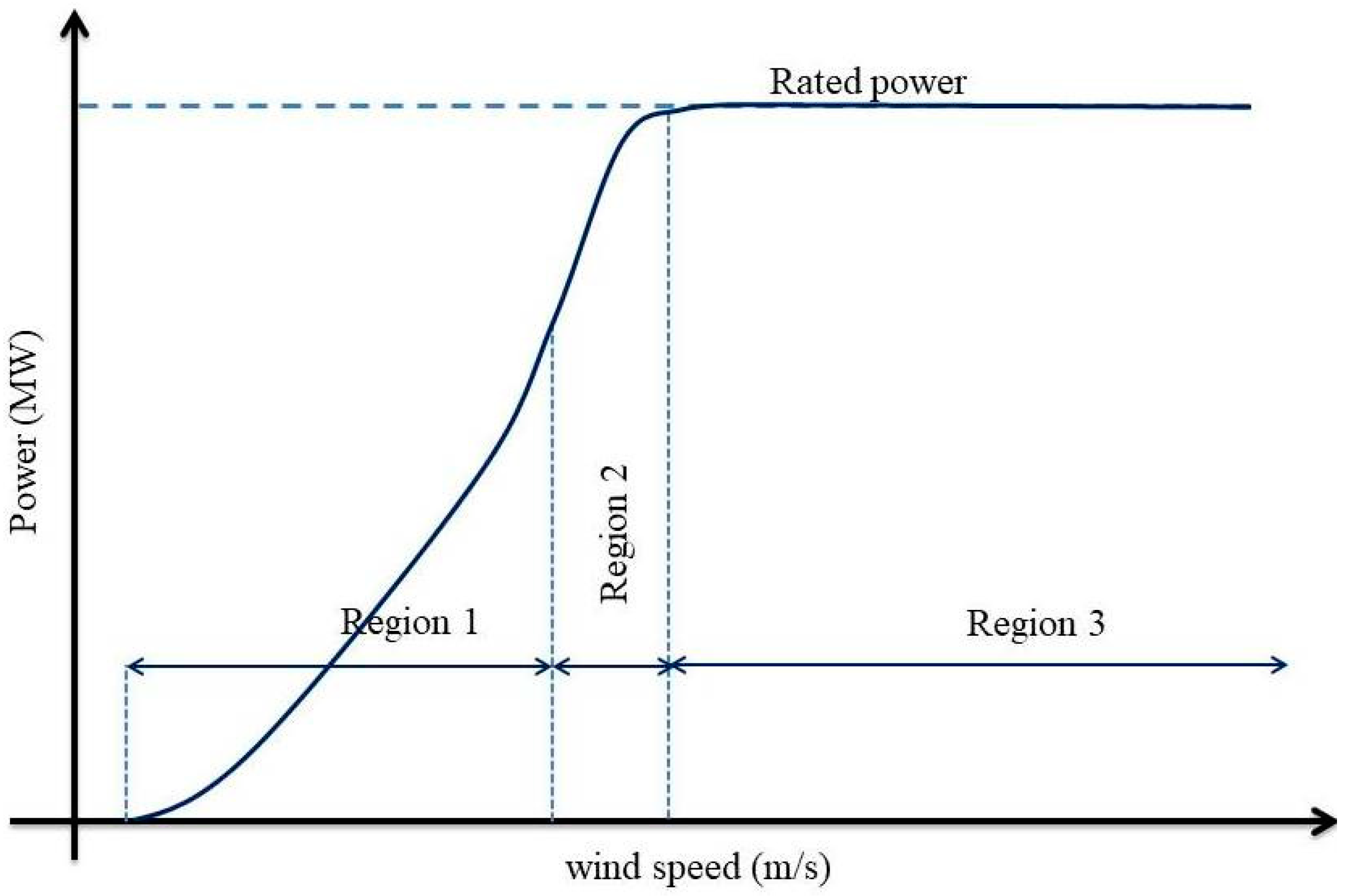
The main objective of this paper is to design a robust adaptive controller to maximize the power extraction from a wind turbine at various operating regions shown in Figure 1. For this purpose, torque control technique is proposed for wind speeds in region one (low wind speeds of range 4−8 m/s) and region two (transition region with medium wind speeds of range 8−11 m/s), and pitch control approach is proposed for wind speeds in region three (high wind speeds of range 11–20 m/s). In all regions, the rotor angular velocity is controlled to maintain the optimum rotor angular speed of the wind turbine. The switching between the regions is enabled based on the wind speed [13].

The next section describes the mathematical modeling of wind turbine dynamics. The third section discusses the methodology used for the design of the adaptive control algorithm for managing wind turbine performance. In the fourth and the fifth sections, the simulations are carried out in Simulink, and results of applying the proposed adaptive control algorithm are presented. The sixth section presents a case study to validate the proposed adaptive control algorithm using real wind speed data. The last section summarizes the results and states the implications and the directions for future research.

2. Wind Turbine Mathematical Modeling

The following mathematical model of the wind turbine system dynamics is based on the work described in [14].

Table 1. Parameters index.

$v$	upstream wind speed (m/s)
$N$	number of blades
$m_t$	mass of tower (kg)
$m_n$	mass of nacelle (kg)
$m_h$	mass of hub (kg)
$m_b$	mass of each blade (kg)
$R_b$	blade radius (m)
$h$	tower height (m)
$d_n$	axial displacement of the nacelle (m)
$\eta$	the angular displacement of the blade (rad)
$S_t$	tower stiffness coefficient (N/m)
$S_b$	blade stiffness coefficient (N/m)
$S_l$	low-speed shaft torsional stiffness coefficient (Nm/rad)
$S_h$	high-speed shaft torsional stiffness coefficient (Nm/rad)
$C_t$	tower damping coefficient (Ns/m)
$C_b$	blade damping coefficient (Ns/m)
$C_l$	low-speed shaft torsional damping coefficient (Nms/rad)
$C_h$	high-speed shaft torsional damping coefficient (Nms/rad)
$J_r$	moment of inertia of elements at ${\omega }_r$ (rotor, blades, shaft, etc.) (kg m2)
$J_g$	moment of inertia of elements at ${\omega }_g$ (generator, shaft, etc.) (kg m2)
$J_w$	equivalent moment of inertia of gearbox elements at ${\alpha }_l$ (kg m2)
${\alpha }_r$	rotor angular position (rad)
${\alpha }_g$	generator angular position (rad)
${\alpha }_l$	the angular position of gearbox low-speed part (rad)
${\alpha }_h$	the angular position of gearbox high-speed part (rad)
${\omega }_r={\dot{\alpha }}_r$	rotor angular speed (rad/s)
${\omega }_g={\dot{\alpha }}_g$	generator angular speed (rad/s)
$T_{wr}$	aerodynamic torque applied by the wind on the rotor (Nm)
$T_g$	antagonistic electrical torque applied on the shaft (Nm)
$T_h$	the torque applied to the gearbox by the high-speed shaft (Nm)
$T_l$	the torque applied to the gearbox by the low-speed shaft (Nm)
$F_w$	thrust force applied by the wind on the rotor (N)
$R_p$	distance from center of the rotor to the center of pressure, or the point where equivalent lumped force $F_w$ is applied
$G_r$	gear ratio

shows the main parameters of the system under consideration. The model development is done by describing the equations of motion and the transfer function of the wind turbine dynamic system.

2.1. Equations of Motion

The equations of motion that govern the wind turbine (WT) dynamics under the effect of wind forces as a function of time are presented in this section. The differential equations that describe the system are expressed in the matrix form. The governing differential equation that describes the whole system could be written as:

$$\left(MM\right)\ddot{u}+\left(CM\right)\dot{u}+\left(SM\right)u=U\left(\dot{u},u,i,t\right)$$

(1)

where $u$ is the vector with the independent variables of the system, $i$ is the input, $t$ is the time, $U$ is the generalized force, $MM$ is the matrix of inertia, $CM$ is the dissipation matrix and $SM$ is the stiffness matrix.

The equations of motion could be expressed as the Euler–Lagrange equation form using the energy-based approach. For this study, the term $K_e$ represents the kinetic energy of the system, $P_e$ the potential energy, $D_{sn}$ is used for the dissipation function of non-conservative forces, while $U_i$ is the conservative generalized forces. $L$ is the Lagrangian function and is defined as $L=K_e-P_e$. Considering this mathematical notation, the Euler–Lagrangian equation could be expressed as:

$$\frac{d}{dt}\left(\frac{\partial L}{\partial {\dot{u}}_n}\right)-\frac{\partial L}{\partial u_n}+\frac{\partial Dsn}{\partial {\dot{u}}_n}=U_{n}n=1,2,\dots ,m_{degreesoffreedom}$$

(2)

2.2. Dynamics of a Doubly Fed Induction Generator Wind Turbine

This model considers a five degree of freedom (rotor angle (${\alpha }_r$), gearbox angle (${\alpha }_l$), generator angle (${\alpha }_g$), blade angular displacement ($\gamma$), and the nacelle axial displacement ($d_n$))system along with the masses of all the main elements of a wind turbine (tower, blades, rotor, gearbox, and generator). The mechanical model considers moment of inertia of the rotor ($J_r$), low-speed gearbox shaft ($J_b$), and generator ($J_g$). The low-speed part of the gearbox has a torsional absorption coefficient of $C_l$, and the stiffness of the low-speed shaft could be expressed by the coefficient $S_l$. The gearbox ratio is represented by $G_r$, and the high-speed part of the gearbox is described by the corresponding stiffness ($C_h$) and the damping ($S_h$) coefficients.

The model presents three main inputs ($f$): the thrust force applied by the wind on the turbine ($F_w$), the torque applied by the wind in the blades ($T_{wr}$), and the electrical torque applied by the generator to compensate the loads on the high-speed shaft ($T_g$). Two important parameters frequently used for optimizing wind turbine performance are the yaw ($\phi$) and the pitch angle ($\varphi$). The following equations are used to describe the doubly fed induction generator (DFIG) wind turbine mechanical modeling.

• Independent variables (u_i):

$$u=\left[u_i\right]={\left[d_n\gamma {\alpha }_r{\alpha }_g{\alpha }_l\right]}^T$$

(3)

• Energy functions (K_e, P_e and D_sn):

The kinetic energy, the potential energy, and the dissipation function of a DFIG wind turbine can be expressed in the following form:

$$K_e=\frac{m_r}{2}{\dot{d_n}}^2+\frac{m_s}{2}(R_b\dot{\eta }+{\dot{d_n)}}^2+\frac{J_r}{2}{\dot{{\alpha }_r}}^2+\frac{J_g}{2}{\dot{{\alpha }_g}}^2+\frac{J_w}{2}{\dot{{\alpha }_l}}^2$$

(4)

$$P_e=\frac{S_t}{2}{d}_n{}^2+\frac{n}{2}{S}_b{(R_b\eta )}^2+\frac{S_l}{2}{({\alpha }_r-{\alpha }_l)}^2+\frac{S_h}{2}{(G_r{\alpha }_l-{\alpha }_g)}^2$$

(5)

$$D_{sn}=\frac{C_t}{2}{\dot{d_n}}^2+\frac{n}{2}{C}_b{(R_b\dot{\eta })}^2+\frac{C_l}{2}{({\dot{\alpha }}_r-{\dot{\alpha }}_l)}^2+\frac{C_h}{2}{(G_r{\dot{\alpha }}_l-{\dot{\alpha }}_g)}^2$$

(6)

where

$${\alpha }_h=G_r{\alpha }_l$$

(7)

$${\dot{\alpha }}_h=G_r{\dot{\alpha }}_l$$

(8)

Applying the Euler–Lagrangian approach to Equations (4)–(6) gives the following equations of motion:

$$\left(m_r+m_s\right){\ddot{d}}_n+m_s{R}_b\ddot{\eta }+S_t{d}_t+C_t{\dot{d}}_t=F_w$$

(9)

$$m_s{R}_b{\ddot{d}}_n+m_s{R}_b^2\ddot{\eta }+n{S}_b{R}_b^2\eta +n{C}_b{R}_b^2\dot{\eta }=R_p{F}_w$$

(10)

$$J_r{\ddot{\alpha }}_r+S_r{\alpha }_r-S_l{\alpha }_l+C_l{\dot{\alpha }}_r-B_l{\dot{\alpha }}_l=T_{wr}$$

(11)

$$J_g{\ddot{\alpha }}_g+S_h{\alpha }_g-S_h{G}_r{\alpha }_l+C_h{\dot{\alpha }}_g-C_h{G}_r{\dot{\alpha }}_l=-T_g$$

(12)

$$J_w{\ddot{\alpha }}_l-S_l{\alpha }_r-S_h{G}_r{\alpha }_g+\left(S_l+S_h{G}_r^2\right){\alpha }_l-C_l{\dot{\alpha }}_r-C_h{G}_r{\dot{\alpha }}_g+\left(C_l+C_h{G}_r^2\right){\dot{\alpha }}_l=0$$

(13)

The above equations of motion from (9) to (13) can be written in matrix form as follows:

$$\left[\begin{array}{ccccc}{m}_r+m_s& m_s{R}_b& 0& 0& 0\\ m_s{R}_b& m_s{R}_b{}^2& 0& 0& 0\\ 0& 0& J_r& 0& 0\\ 0& 0& 0& J_g& 0\\ 0& 0& 0& 0& J_w\end{array}\right]\left[\begin{array}{c}{\ddot{d}}_n\\ \ddot{\eta }\\ {\ddot{\alpha }}_r\\ {\ddot{\alpha }}_g\\ {\ddot{\alpha }}_l\end{array}\right]=\left(MM\right)\ddot{u}$$

(14)

$$\left[\begin{array}{ccccc}{C}_t& 0& 0& 0& 0\\ 0& n{C}_b{R}_b{}^2& 0& 0& 0\\ 0& 0& C_l& 0& -C_l\\ 0& 0& 0& C_h& -C_h{G}_r\\ 0& 0& -C_l& -S_h{G}_r& C_l+C_h{G}_r{}^2\end{array}\right]\left[\begin{array}{c}{\dot{d}}_n\\ \dot{\eta }\\ {\dot{\alpha }}_r\\ {\dot{\alpha }}_g\\ {\dot{\alpha }}_l\end{array}\right]=\left(CM\right)\dot{u}$$

(15)

$$\left[\begin{array}{ccccc}{S}_t& 0& 0& 0& 0\\ 0& n{S}_b{R}_b{}^2& 0& 0& 0\\ 0& 0& S_l& 0& -S_l\\ 0& 0& 0& S_h& -S_h{G}_r\\ 0& 0& -S_l& -S_h{G}_r& S_l+S_h{G}_r{}^2\end{array}\right]\left[\begin{array}{c}{d}_n\\ \eta \\ {\alpha }_r\\ {\alpha }_g\\ {\alpha }_l\end{array}\right]=\left(SM\right)u$$

(16)

$$U=\left[\begin{array}{c}{F}_w\\ R_p{F}_w\\ T_{wr}\\ -T_s\\ 0\end{array}\right]=\left[\begin{array}{ccc}1& 0& 0\\ R_p& 0& 0\\ 0& 1& 0\\ 0& 0& -1\\ 0& 0& 0\end{array}\right]\left[\begin{array}{c}{F}_w\\ T_{wr}\\ T_g\end{array}\right]=\left(RM\right)f$$

(17)

Using Equation (1) and Equations (14)–(17), the following equation can be derived:

$$\ddot{u}=-{\left(MM\right)}^{-1}\left(CM\right)\dot{u}-{\left(MM\right)}^{-1}\left(SM\right)u+{\left(MM\right)}^{-1}\left(RM\right)f$$

(18)

• State-space system description: the following vectors are established for the state-space system representation:

$$\mathrm{State}\mathrm{variables}:\mathit{x}={\left[\begin{array}{cccccccccc}{d}_n& \eta & {\alpha }_r& {\alpha }_g& {\alpha }_l& {\dot{d}}_n& \dot{\eta }& {\dot{\alpha }}_r& {\dot{\alpha }}_g& {\dot{\alpha }}_l\end{array}\right]}^T$$

(19)

$$\mathrm{Inputs}:\mathit{f}={\left[\begin{array}{ccc}{F}_w& T_{wr}& T_g\end{array}\right]}^T$$

(20)

$$\mathrm{Outputs}:\mathit{y}={\left[\begin{array}{ccccc}{\dot{d}}_n& \dot{\eta }& {\dot{\alpha }}_r& {\dot{\alpha }}_g& {\dot{\alpha }}_l\end{array}\right]}^T$$

(21)

Equation (18) could be re-written in the traditional state-space representation form:

$$\begin{array}{c}\dot{x}=\left(AM\right)x+\left(BM\right)u\\ y=\left(DM\right)x\end{array}$$

(22)

Applying the state-space representation to the system, the following equation is obtained:

$$\begin{array}{c}{\dot{x}}_{10\times 1}=\left[\begin{array}{cc}{0}_{5\times 5}& I_{5\times 5}\\ -M{M}_{5\times 5}^{-1}S{M}_{5\times 5}& -M{M}_{5\times 5}^{-1}C{M}_{5\times 5}\end{array}\right]x_{10\times 1}+\left[\begin{array}{c}{0}_{5\times 3}\\ -M{M}_{5\times 5}^{-1}R{M}_{5\times 3}\end{array}\right]u_{3\times 1}\\ y=\left[\begin{array}{cc}{0}_{5\times 5}& I_{5\times 5}\end{array}\right]x_{10\times 1}\end{array}$$

(23)

where Equation (23) is a system of three inputs and five outputs. The following is the representation of ${(MM)}^{-1}$ matrix:

$${\left(MM\right)}^{-1}=\left[\begin{array}{ccccc}\frac{1}{m_r}& \frac{-1}{m_r{R}_b}& 0& 0& 0\\ \frac{-1}{m_r{R}_b}& \frac{m_r+m_s}{m_r{m}_s{R}_b^2}& 0& 0& 0\\ 0& 0& \frac{1}{J_r}& 0& 0\\ 0& 0& 0& \frac{1}{J_g}& 0\\ 0& 0& 0& 0& \frac{1}{J_w}\end{array}\right]$$

(24)

Finally, the state-space representation matrices could be written as:

$$AM=\left[\begin{array}{cccccccccc}0& 0& 0& 0& 0& 1& 0& 0& 0& 0\\ 0& 0& 0& 0& 0& 0& 1& 0& 0& 0\\ 0& 0& 0& 0& 0& 0& 0& 1& 0& 0\\ 0& 0& 0& 0& 0& 0& 0& 0& 1& 0\\ 0& 0& 0& 0& 0& 0& 0& 0& 0& 1\\ -\frac{S_t}{m_r}& \frac{n{S}_b{R}_b}{m_r}& 0& 0& 0& -\frac{C_t}{m_r}& -\frac{n{C}_b{R}_b}{m_r}& 0& 0& 0\\ \frac{S_t}{m_r{R}_b}& -\frac{(m_r+m_s)n{S}_b}{m_r{m}_s}& 0& 0& 0& \frac{C_t}{m_r{R}_b}& -\frac{(m_r+m_s)n{C}_b}{m_r{m}_s}& 0& 0& 0\\ 0& 0& -\frac{S_l}{J_r}& 0& \frac{S_l}{J_r}& 0& 0& -\frac{C_l}{J_r}& 0& \frac{C_l}{J_r}\\ 0& 0& 0& -\frac{S_h}{J_g}& \frac{S_h{G}_r}{J_g}& 0& 0& 0& -\frac{C_h}{J_g}& \frac{C_h{G}_r}{J_g}\\ 0& 0& \frac{S_l}{J_w}& \frac{S_h{G}_r}{J_w}& -\frac{S_l+S_h{R}_t^2}{J_w}& 0& 0& \frac{C_l}{J_w}& \frac{C_h{G}_r}{J_w}& -\frac{C_l+C_h{R}_t^2}{J_w}\end{array}\right]$$

(25)

$$BM=\left[\begin{array}{ccc}0& 0& 0\\ 0& 0& 0\\ 0& 0& 0\\ 0& 0& 0\\ 0& 0& 0\\ \frac{1}{m_r}\left(1-\frac{R_p}{R_b}\right)& 0& 0\\ \frac{1}{m_r{R}_b}\left(\frac{\left(m_r+m_s\right)R_p}{m_s{R}_b}-1\right)& 0& 0\\ 0& \frac{1}{J_r}& 0\\ 0& 0& -\frac{1}{J_g}\\ 0& 0& 0\end{array}\right]$$

(26)

$$DM=\left[\begin{array}{cccccccccc}0& 0& 0& 0& 0& 1& 0& 0& 0& 0\\ 0& 0& 0& 0& 0& 0& 1& 0& 0& 0\\ 0& 0& 0& 0& 0& 0& 0& 1& 0& 0\\ 0& 0& 0& 0& 0& 0& 0& 0& 1& 0\\ 0& 0& 0& 0& 0& 0& 0& 0& 0& 1\end{array}\right]$$

(27)

2.3. Wind Turbine Transfer Matrix

Using the state-space matrices, the transfer function matrix is obtained that represents the system dynamics:

$$P\left(s\right)=\left(CM\right){\left(sI-\left(AM\right)\right)}^{-1}\left(BM\right),\mathrm{for}y\left(s\right)=P\left(s\right)f\left(s\right)$$

(28)

The system outputs are described as:

$$y\left(s\right)=\left[\begin{array}{c}{\dot{d}}_t\left(s\right)\\ \dot{\eta }\left(s\right)\\ {\omega }_r\left(s\right)\\ {\omega }_g\left(s\right)\\ {\omega }_l\left(s\right)\end{array}\right]=\left[\begin{array}{ccc}{g}_{11}\left(s\right)& 0& 0\\ g_{21}\left(s\right)& 0& 0\\ 0& g_{32}\left(s\right)& g_{33}\left(s\right)\\ 0& g_{42}\left(s\right)& g_{43}\left(s\right)\\ 0& g_{52}\left(s\right)& g_{53}\left(s\right)\end{array}\right]\left[\begin{array}{c}{F}_w\left(s\right)\\ T_{wr}\left(s\right)\\ T_g\left(s\right)\end{array}\right]=P\left(s\right)f\left(s\right)$$

(29)

where the inner terms of the transfer function matrix could be described as:

$$g_{ij}\left(s\right)=\frac{g_{n_{ij}}\left(s\right)}{g_{d_{ij}}\left(s\right)}\mathrm{for}i=1,2,3,4,5;j=1,2,3$$

(30)

$$g_{n_{11}}\left(s\right)=\left[s^2\left(m_s\left(R_b-R_p\right)\right)+s\left(n{C}_b{R}_b\right)+n{S}_b{R}_b\right]s$$

(31)

$$g_{d_{11}}\left(s\right)=\left[s^4\left(m_r{m}_s\right)+s^3(m_{s}n{C}_b+m_s{C}_t+m_{r}n{C}_b)+s^2(m_s{S}_t+n{C}_t{C}_b+m_{r}n{S}_b+m_{s}n{S}_b)+s(n{C}_t{S}_b+n{C}_b{S}_t)+\left(n{S}_t{S}_b\right)\right]R_b$$

(32)

$$g_{n_{21}}\left(s\right)=\left[s^2\left(m_s\left(R_b-R_p\right)+m_r{R}_p\right)+s\left(C_t{R}_p\right)+S_t{R}_p\right]s$$

(33)

$$g_{d_{21}}\left(s\right)=g_{d_{11}}\left(s\right)R_b$$

(34)

$$g_{n_{32}}\left(s\right)=s^4\left(J_g{J}_w\right)+s^3(J_w{C}_h+J_g{C}_l+J_g{C}_h{G}_r{}^2)+s^2(C_l{C}_h+J_g{S}_l+J_g{S}_h{G}_r{}^2+J_w{S}_h)+s(C_l{S}_h+C_h{S}_l)+\left(S_h{S}_l\right)$$

(35)

$$g_{d_{32}}\left(s\right)=\left[s^4\left(J_g{J}_w{J}_r\right)+s^3(J_r{J}_g{C}_l+J_r{J}_w{C}_h+J_r{J}_g{C}_h{G}_r{}^2+J_g{J}_w{C}_l)+s^2(S_l{J}_g{J}_w+C_h{J}_r{C}_l+C_l{J}_g{C}_h{G}_r{}^2+J_r{J}_w{S}_h+J_r{J}_g{S}_l+C_h{J}_w{C}_l+J_r{J}_g{S}_h{G}_r{}^2)+s(C_l{S}_h{J}_w+C_h{S}_l{J}_g{G}_r{}^2+C_l{S}_h{J}_r+C_h{S}_l{J}_r+C_h{S}_l{J}_w+C_l{S}_h{J}_g{G}_r{}^2)+(S_l{S}_h{J}_g{G}_r{}^2+S_h{S}_l{J}_r+S_h{S}_l{J}_w)\right]s$$

(36)

$$g_{n_{33}}\left(s\right)=-s^2\left(C_h{C}_l{G}_r\right)-s\left[G_r\left(C_l{S}_h+C_h{S}_l\right)\right]-\left(S_h{S}_l{G}_r\right)$$

(37)

$$g_{d_{33}}\left(s\right)=g_{d_{32}}\left(s\right)$$

(38)

$$g_{n_{42}}\left(s\right)=-g_{n_{33}}\left(s\right)$$

(39)

$$g_{d_{42}}\left(s\right)=g_{d_{32}}\left(s\right)$$

(40)

$$g_{n_{43}}\left(s\right)=-s^4\left(J_r{J}_w\right)+s^3(J_r{C}_l+J_w{C}_l+J_r{C}_h{G}_r{}^2)-s^2(C_l{C}_h{G}_r{}^2+J_r{S}_l+J_r{S}_h{G}_r{}^2+J_w{S}_l)-s(C_l{S}_h{G}_r{}^2+C_h{S}_l{G}_r{}^2)-\left(S_h{S}_l{G}_r{}^2\right)$$

(41)

$$g_{d_{43}}\left(s\right)=g_{d_{32}}\left(s\right)$$

(42)

$$g_{n_{52}}\left(s\right)=s^3\left(J_g{C}_l\right)+s^2\left(C_l{C}_h+J_g{S}_l\right)+s\left(C_l{S}_h+C_h{S}_l\right)+\left(S_h{S}_l\right)$$

(43)

$$g_{d_{52}}\left(s\right)=g_{d_{32}}\left(s\right)$$

(44)

$$g_{n_{53}}\left(s\right)=-s^3\left(J_r{C}_h{G}_r\right)-s^2\left[G_r\left(J_r{S}_h+C_h{C}_l\right)\right]-s\left[G_r\left(C_l{S}_h+C_h{S}_l\right)\right]-\left(S_h{S}_l{G}_r\right)$$

(45)

$$g_{d_{53}}\left(s\right)=g_{d_{32}}\left(s\right)$$

(46)

$${\omega }_r\left(s\right)=g_{32}\left(s\right)T_{wr}\left(s\right)+g_{33}\left(s\right)T_g\left(s\right)$$

(47)

Considering the inputs of the transfer function, according to the equations developed for the study of wind turbine aerodynamics, the thrust force ($F_w$) applied by the wind on the rotor blades and the aerodynamic torque ($T_{wr}$) that the air exerts on the wind turbine rotor are expressed as:

$$F_w=\frac{1}{2}{\rho }_{air}\pi R_b{}^2{C}_T\left(\lambda ,\varphi \right)v^2$$

(48)

$$T_{wr}=\frac{{\rho }_{air}\pi R_b{}^2{C}_P\left(\lambda ,\varphi \right)v^3}{2{\omega }_r}$$

(49)

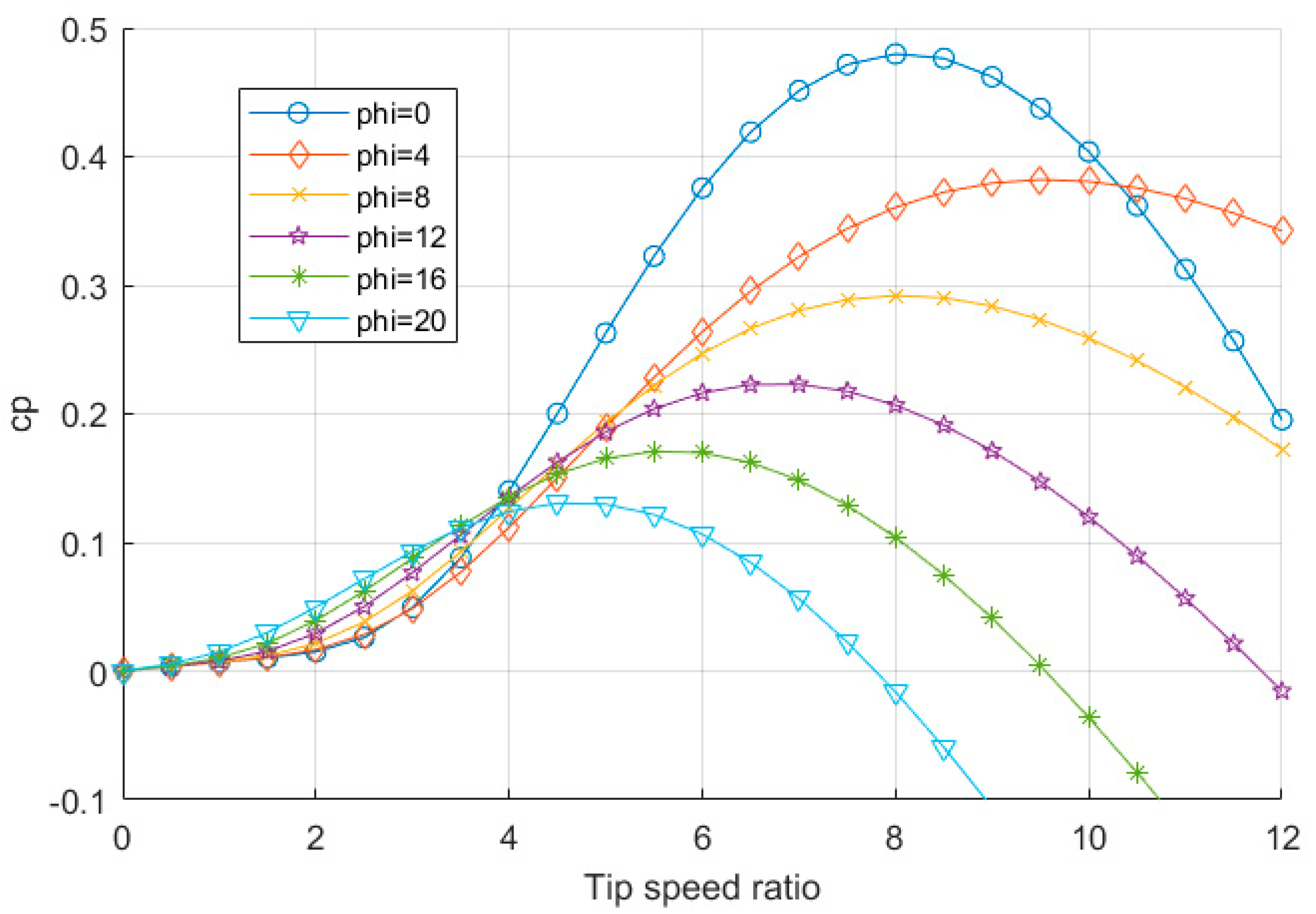
where ${\rho }_{air}$ is the density of the air,$C_T$ and $C_P$ are the thrust and the aerodynamic power coefficients as a function of pitch angle, $\varphi ,$ and tip speed ratio, $\lambda =\frac{{\omega }_r{R}_b}{v}$, respectively. The power coefficient is the product of aerodynamic torque coefficient $(C_Q$) and tip speed ratio ($\lambda$), and the numerical approximation of the aerodynamic power coefficient (Figure 2) is given by the following equation:

$$C_P\left(\lambda ,\varphi \right)=a1\left(\frac{a2}{{\lambda }_i}-a3\varphi -a4\right)e^{-\frac{a5}{{\lambda }_i}}+a6\lambda$$

(50)

where $\frac{1}{{\lambda }_i}=\frac{1}{\lambda +a7\varphi }-\frac{a8}{{\varphi }^3+1}$ and the coefficient values according to [10] are $a1$= 0.5176, $a2$ = 116, $a3$ = 0.4, $a4$ = 5, $a5$ = 21, $a6$ = 0.0068, $a7$ = 0.09, $a8$ = 0.035.

The wind turbine plant transfer functions for pitch control $g_{32}\left(s\right)$ and torque control $g_{33}\left(s\right)$ for the 2 MW and the 5 MW wind turbines are as follows:

$$g_{32}\left(s\right)=\frac{g_{n_{32}}\left(s\right)}{g_{d_{32}}\left(s\right)}=\frac{s^4\left(J_g{J}_w\right)+s^3\left(J_w{C}_h+J_g{C}_l+J_g{C}_h{G}_r{}^2\right)+\cdots \cdots }{s^5\left(J_g{J}_w{J}_r\right)+s^4\left(J_r{J}_g{C}_l+J_r{J}_w{C}_h+J_r{J}_g{C}_h{G}_r{}^2+J_g{J}_w{C}_l\right)+\cdots \cdots }$$

(51)

$$g_{33}\left(s\right)=\frac{g_{n_{33}}\left(s\right)}{g_{d_{33}}\left(s\right)}=\frac{-s^2\left(C_h{C}_l{G}_r\right)-s\left[G_r\left(C_l{S}_h+C_h{S}_l\right)\right]+\cdots \cdots }{s^5\left(J_g{J}_w{J}_r\right)+s^4\left(J_r{J}_g{C}_l+J_r{J}_w{C}_h+J_r{J}_g{C}_h{G}_r{}^2+J_g{J}_w{C}_l\right)+\cdots \cdots }$$

(52)

It should be noted that only the values of the parameters change for 2 MW and 5 MW wind turbines, and the transfer functions remain the same. The same transfer function is used for the case study in Section 6. The 2 MW and the 5 MW wind turbine parameters used for the simulation are of doubly-fed induction generator wind turbines [14,15] as given in

Table 2. Wind turbine parameters.

Parameter	2 MW	5 MW
Cut-in wind speed	4 m/s	3 m/s
Rated wind speed	11 m/s	11 m/s
$\mathrm{Mass}\mathrm{of}\mathrm{hub}\mathrm{and}\mathrm{nacelle}(m_n+m_h)$	75,080 kg	296,780 kg
$\mathrm{Mass}\mathrm{of}\mathrm{each}\mathrm{blade}\left(m_b\right)$	4490 kg	17,740 kg
$\mathrm{Mass}\mathrm{of}\mathrm{the}\mathrm{tower}\left(m_t\right)$	87,900 kg	347,460 kg
$\mathrm{Radius}\mathrm{of}\mathrm{blade}\left(R_b\right)$	40 m	61.5 m
$\mathrm{Rotor}\mathrm{moment}\mathrm{of}\mathrm{inertia}\left(J_r\right)$	5.5 × 106 kg m2	3.5 × 107 kg m2
$\mathrm{Low}-\mathrm{speed}\mathrm{shaft}\mathrm{torsional}\mathrm{damping}\mathrm{coefficient}\left(C_l\right)$	25,000 Nms/rad	1000 Nms/rad
$\mathrm{High}-\mathrm{speed}\mathrm{shaft}\mathrm{torsional}\mathrm{damping}\mathrm{coefficient}\left(C_h\right)$	36 Nms/rad	1 Nms/rad
$\mathrm{Gear}\mathrm{ratio}\left(G_r\right)$	83.33	97
$\mathrm{Tower}\mathrm{damping}\mathrm{coefficient}\left(C_t\right)$	7590 Ns/m	18,970 Ns/m
$\mathrm{Blade}\mathrm{damping}\mathrm{coefficient}\left(C_b\right)$	50 Ns/m	125 Ns/m
$\mathrm{Blade}\mathrm{stiffness}\mathrm{coefficient}\left(S_b\right)$	21,840 N/m	54,590 N/m
$\mathrm{Tower}\mathrm{stiffness}\mathrm{coefficient}\left(S_t\right)$	772,200 N/m	1,930,490 N/m
$\mathrm{Low}-\mathrm{speed}\mathrm{shaft}\mathrm{torsional}\mathrm{stiffness}\mathrm{coefficient}\left(S_l\right)$	1.6 × 108 Nm	7.63 × 109 Nm
$\mathrm{High}-\mathrm{speed}\mathrm{shaft}\mathrm{torsional}\mathrm{stiffness}\mathrm{coefficient}\left(S_h\right)$	2.3 × 104 Nm	3.5 × 105 Nm
$\mathrm{Generator}\mathrm{moment}\mathrm{of}\mathrm{inertia}\left(J_g\right)$	60 kg m2	530 kg m2
$\mathrm{Maximum}\mathrm{generator}\mathrm{torque}(T_{g_{max}}$)	14,000 Nm	47,000 Nm
$\mathrm{Nominal}\mathrm{rotor}\mathrm{speed}\left({\omega }_{r_{nominal}}\right)$	2 rad/s	1.27 rad/s

.

3. Adaptive Control Algorithm

This section focuses on the formulation and the design of a simple direct adaptive control algorithm [16]. Consider the linear time-invariant plant:

$${\dot{x}}_p=A_p{x}_p+B_p{u}_p\hspace{1em}\mathrm{and}\hspace{1em}{y}_p=C_p{x}_p$$

(53)

where $A_p$ and $B_p$ are plant matrices, $x_p$ is the state vector, $u_p$ is the control vector, and $y_p$ is the plant output vector. Elements of $A_p$ and $B_p$ are assumed to be bounded between some upper ($u$) and lower ($l$) bounds:

$${\left(a_{ij}\right)}_l\le a_p\left(i,j\right)\le {\left(a_{ij}\right)}_u\hspace{1em};\hspace{1em}{\left(b_{ij}\right)}_l\le b_p\left(i,j\right)\le {\left(b_{ij}\right)}_u$$

(54)

where $a_p\left(i,j\right)$ and $b_p\left(i,j\right)$ are the ${\left(i,j\right)}^{th}$ elements of $A_p$ and $B_p,$ respectively.

The main objective here is to find a control $u_p$ without explicit knowledge of $A_p$ and $B_p$ that follows the output of the following reference model:

$$\begin{array}{c}{\dot{x}}_m=A_m{x}_m+B_m{u}_m\\ y_m=C_m{x}_m\end{array}$$

(55)

The model has desired plant behavior. However, the model choice is not restricted. The order of the plant may be much larger compared to the reference model such that:

$$\dim \left[x_p\right]\gg \dim \left[x_m\right]$$

(56)

The reference model must have the same number of outputs as the plant. The adaptive control signal composed of the error in the feedback, the model states, and the model input in the feed-forward, as shown in Figure 3, is given below:

$$u_p\left(t\right)=K_e\left(t\right)\left[y_m\left(t\right)-y_p\left(t\right)\right]+K_x\left(t\right)x_m\left(t\right)+K_u\left(t\right)u_m\left(t\right)$$

(57)

where $K_e\left(t\right)$, $K_x\left(t\right)$, $K_u\left(t\right)$ are adaptive gains on error, model state, and model input, respectively, and ($y_m\left(t\right)-y_p\left(t\right)$) is the output error, also denoted as $e_y\left(t\right)$.

The adaptive gain is the sum of proportional gain $K_P$ and integral gain $K_I,$ which are written as follows:

$$K_e=K_{Ie}+K_{Pe}$$

(58)

$$K_x=K_{Ix}+K_{Px}$$

(59)

$$K_u=K_{Iu}+K_{Pu}$$

(60)

where:

$${\dot{K}}_{Ie}=e_y{e}_y^T{T}_{Ie}-\sigma K_{Ie},\hspace{1em}{T}_{Ie}>0$$

(61)

$$K_{Pe}=e_y{e}_y^T{T}_{Pe},\hspace{1em}\hspace{1em}{T}_{Pe}\ge 0$$

(62)

$${\dot{K}}_{Ix}=e_y{x}_m^T{T}_{Ix}-\sigma K_{Ix},T_{Ix}>0$$

(63)

$$K_{Px}=e_y{x}_m^T{T}_{Px},\hspace{1em}\hspace{1em}{T}_{Px}\ge 0$$

(64)

$${\dot{K}}_{Iu}=e_y{u}_y^T{T}_{Iu}-\sigma K_{Iu},T_{Iu}>0$$

(65)

$$K_{Pu}=e_y{u}_m^T{T}_{Pu},\hspace{1em}\hspace{1em}{T}_{Pu}\ge 0$$

(66)

where $T_{Pe}$, $T_{Pu}$ and $T_{Px}$ are time-invariant weighting matrices for proportional gains. $T_{Ie}$, $T_{Ix}$ and $T_{Iu}$ are the time-invariant weighting matrices for integral gains, and $\sigma$ takes values between 0.05 and 0.1.

For asymptotic tracking, the plant must be almost strictly positive real (ASPR), which means there exists a positive definite gain matrix $K$ not needed for implementation such that the closed-loop transfer function:

$$G\left(s\right)={\left[I+P\left(s\right)K\right]}^{-1}P\left(s\right)$$

(67)

is strictly positive real (SPR). $P\left(s\right)$ is the transfer function of the plant in consideration and is ASPR if (a) it is a minimum phase, (b) it has a relative degree of one or zero, (c) it has a positive definite high-frequency gain. In general, most physical plants may not satisfy the ASPR conditions due to the restrictive nature. Such plants of the form $P\left(s\right)=\left(CM\right){\left(sI-\left(AM\right)\right)}^{-1}\left(BM\right)$ given in Equation (28) can be made ASPR with augmentation of a feed-forward compensator $H\left(s\right)$ [16].

$$G_a\left(s\right)=P\left(s\right)+H\left(s\right)=\frac{N_a\left(s\right)}{D_a\left(s\right)}$$

(68)

where $G_a\left(s\right)$ is the augmented ASPR plant transfer function.

Compensator Design

To implement the adaptive control algorithm, the wind turbine plant transfer function must be ASPR, as mentioned above. In region three for the pitch control, the wind turbine plant transfer function for 2 MW and 5 MW given in Equation (51) is ASPR because the relative degree is one, it is a minimum phase, and it has a positive definite high-frequency gain. Hence, there is no need to design a compensator for pitch control. In regions one and two for the torque control, the wind turbine plant transfer function for 2 MW and 5 MW shown in Equation (52) is non-ASPR because it does not satisfy the relative degree condition. In order to make the plant transfer function as an ASPR, a feed-forward compensator has to be augmented in parallel to the plant transfer function.

Assume a non-ASPR plant of the form:

$$P\left(s\right)=\frac{C_m{s}^m+C_{m-1}{s}^{m-1}+C_{m-2}{s}^{m-2}+\cdots \cdots \cdots +C_0}{D_n{s}^n+D_{n-1}{s}^{n-1}+D_{n-2}{s}^{n-2}+\cdots \cdots \cdots +D_0}$$

(69)

where the coefficients $C_{m-k}$ and $D_{n-k}$ can take any values within the given upper (u) bound and lower (l) bound:

$$\begin{gathered} {(C_{m-k})}_u\le C_{m-k}\le {(C_{m-k})}_{l}k=0,1,2\cdots ,m \\ {(D_{n-k})}_u\le D_{n-k}\le {(D_{n-k})}_{l}k=0,1,2\cdots ,n \end{gathered}$$

(70)

It is also assumed that the nominal plant parameters, the upper bound and the lower bound values of the plant, along with the degrees (m, n) are known. The feed-forward compensator is selected such that it has the same order (n) as that of the plant.

$$H\left(s\right)=\frac{f_{n-1}{s}^{n-1}+f_{n-2}{s}^{n-2}+f_{n-3}{s}^{n-3}+\cdots \cdots \cdots +f_0}{s^n+h_{n-1}{s}^{n-1}+h_{n-2}{s}^{n-2}+\cdots \cdots \cdots +h_0}$$

(71)

This compensator will always satisfy the relative degree condition. The denominator coefficients of $H\left(s\right)$ are determined in a way to make the compensator time constant faster than the reference model because of the condition that the feed-forward compensator transients should be much faster than the reference model transients. The numerator polynomial coefficients, which guarantee the stability of the closed-loop characteristic equation, are found using an optimization algorithm as discussed below:

$$\begin{array}{c}minimize\{{\displaystyle \sum }{f}_i^2\}\\ subto:max\left\{Real\left[roots\left(N_a\left(s\right)\right)\right]\right\}<0\end{array}$$

(72)

where $f_i$ is the coefficient of numerator polynomial of the compensator, and $N_a\left(s\right)$ is the numerator polynomial of the augmented plant transfer function, as given in Equation (68). The optimization is carried out using the $fmincon$ command in the MATLAB. The objective function is the summation of squares of the coefficients of numerator polynomial of the compensator $f_i$. The constraints for the optimization are applied using 2 MW parameters as lower bound and 5 MW parameters as upper bound. From the optimization, the coefficients are extracted, and the compensator is designed, which makes the plant ASPR. In the following section, the compensator designed for the plant is given along with the parameter values used for the simulation.

4. Simulation

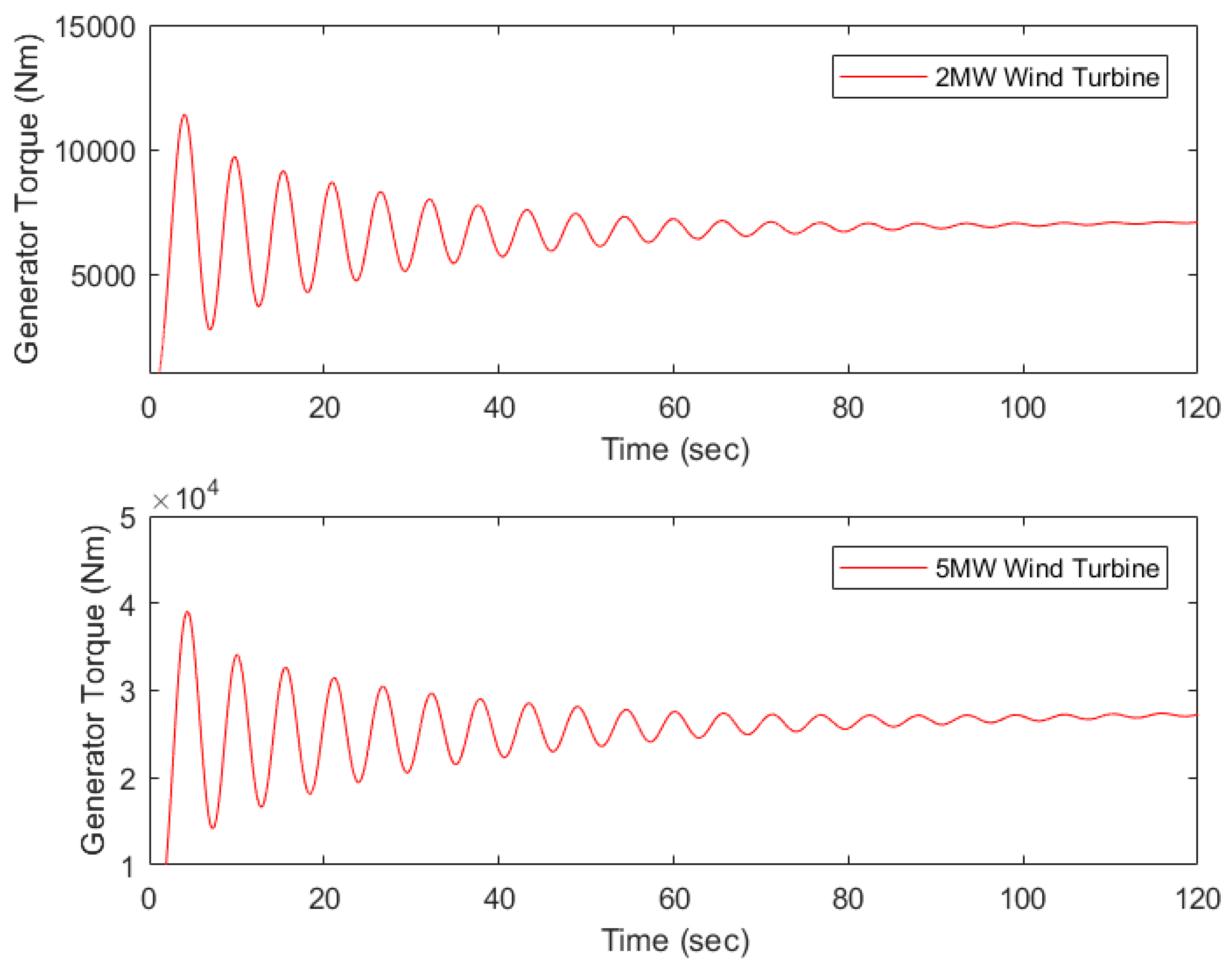
The adaptive control model is designed and implemented on the 2 MW and the 5 MW wind turbine models using MATLAB/Simulink software to analyze the performance and the stability of the higher-order dynamic system of the wind turbine. It is important to note that the same compensator model is used for the 2 MW and the 5 MW wind turbine plants. The simulation is done to verify the rotor speed tracking performance of the designed adaptive control strategy. The wind turbine plant adaptive controller block diagram is as shown in Figure 4. The torque controller is enabled when the wind speed is less than the rated wind speed for region one and region two, where the rotor angular speed is controlled to optimize the aerodynamic efficiency by varying the generator torque (T_g). The pitch controller is enabled when the wind speed is equal to or greater than the rated wind speed for region three, where the rotor speed is controlled to extract the rated wind power, reduce the aerodynamic loads due to high turbulent wind speeds, and maintain the structural safety by varying the pitch angle, phi ($\mathsf{\varphi }$).

The feed-forward compensator initially found as below in Equation (73) has the same order as the plant for the simplicity of calculations. The denominator of the compensator is predetermined such that the compensator poles are much farther from the poles of the plant to eliminate any effects at a steady state or let the transients of the compensator diminishes quickly.

$$H\left(s\right)=\frac{f_4{s}^4+f_3{s}^3+f_2{s}^2+f_{1}s+f_0}{\left(s+3\right)\left(s+4\right)\left(s+6\right)\left(s+9\right)\left(s+15\right)}$$

(73)

The numerator polynomial coefficients are determined using the procedure as discussed in Equation (72). The optimization algorithm returns the following values for the numerator polynomial coefficients, as shown in

Table 3. Compensator numerator coefficients.

Parameter	${\mathit{f}}_4$	${\mathit{f}}_3$	${\mathit{f}}_2$	${\mathit{f}}_1$	${\mathit{f}}_0$
Value	30	30	63.728	36.973	30

.

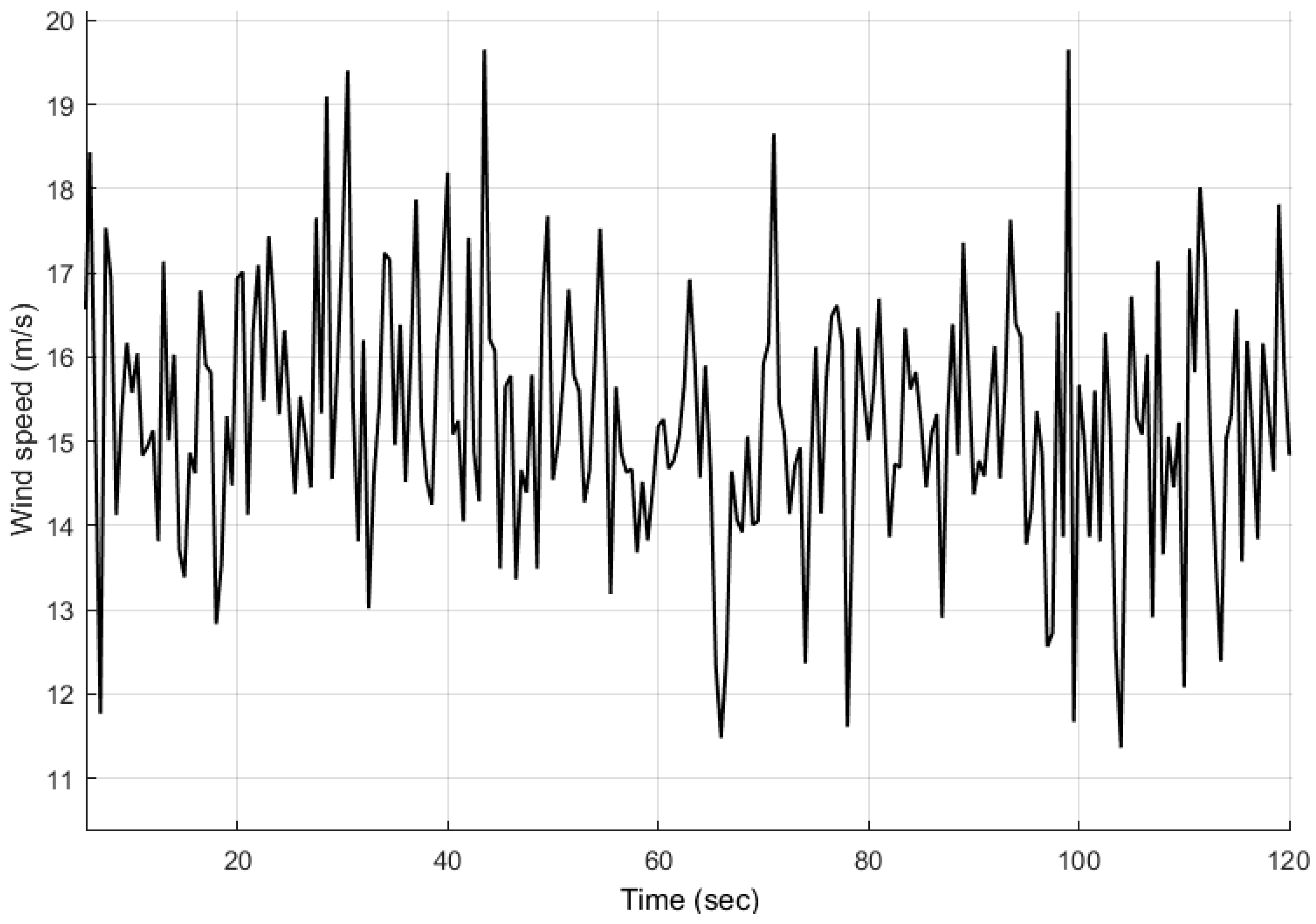
Wind speed distribution used for the simulation is approximated by using Gaussian probability density function [17] given by:

$$f\left(v\right)=\frac{1}{\sigma \sqrt{2\pi }}{\mathrm{e}}^{\left(\frac{-{\left(v-v_m\right)}^2}{2{\sigma }^2}\right)}$$

(74)

where $v$ is the wind speed, $v_m$ is the mean wind speed, and $\sigma$ is the standard deviation of wind speed. The time-invariant weights $T_{Pe}$, $T_{Pu}$, and $T_{Px}$ for proportional gains and $T_{Ie}$, $T_{Ix,}$ and $T_{Iu}$ for integral gains used for the simulation are given in

Table 4. Weights for the adaptive gains.

Parameter	Value	Parameter	Value
$T_{Pe}$	1	$T_{Ie}$	1
$T_{Pu}$	104	$T_{Ix}$	1
$T_{Px}$	104	$T_{Iu}$	104

.

It is important to note that the weights of the adaptive gains remain the same for all the cases of simulation and still could give a satisfactory tracking of the output. The next section presents the results obtained from the simulation done in MATLAB/Simulink for pitch control, torque control, and combined control for the 2 MW and the 5 MW wind turbines.

5. Results and Discussion

The proposed adaptive control is designed and successfully implemented on the two wind turbine models, and the performance characteristics are analyzed using MATLAB/Simulink. The results of the three cases for the two wind turbines based on wind speed are discussed in this section. For all cases, a first-order transfer function is used as a reference model. The nominal value of the rotor speed is given as the input to the reference model. The reference angular speed of the rotor is the output from the reference model, which is fed as input to the controller, as shown in Figure 4. This enables the controller to track the optimal angular speed of the rotor.

5.1. Pitch Control

For the pitch control case, the wind speed is assumed to be above-rated wind speed (11 m/s) and below the cut-off wind speed (20 m/s). The wind speed distribution for this case is approximated using the mean wind speed as 16 m/s with a standard deviation of 2. The adaptive control varies the pitch angle based on the error value between the reference rotor speed (${\omega }_{r\_ref}$) and the rotor speed (${\omega }_r$) from the plant. The plant output in this region is calculated for varying pitch angles by considering the generator torque as a constant value. The wind speed profile for region three is as given in Figure 5. This wind speed is given as disturbance input to the plant for both the 2 MW and the 5 MW wind turbines.

The rotor speed regulation of the 2 MW and the 5 MW wind turbines in the pitch control region are shown in Figure 6. It can be seen that the rotor speed follows the reference rotor speed as close as possible to the values, 2 rad/s for 2 MW wind turbine and 1.27 rad/s for the 5 MW wind turbine. The pitch angle variations and $C_P$ for 2 MW and 5 MW wind turbines are shown in Figure 7. The adaptive control varies the pitch angle to limit the aerodynamic torque at the rotor. The performance of the adaptive control in tracking the rotor speed is satisfactory with no steady-state error for both types of wind turbines. This enables the aerodynamic efficiency of the wind turbine to be optimum in this high wind speed region, which can be seen in the $C_P$ graph with the mean value of 0.45.

5.2. Torque Control

For the torque control case, the wind speed is assumed to be between the cut-in wind speed (4 m/s) and rated wind speed (11 m/s). The disturbance input of the plant is approximated using the mean wind speed as 8 m/s with a standard deviation of two. In this case, the adaptive control varies the generator torque based on the error value between the reference rotor speed (${\omega }_{r\_ref}$) and the rotor speed (${\omega }_r$) from the plant. The plant output is calculated for varying generator torque by maintaining the pitch angle as zero. The wind speed distribution for torque control region is as depicted in Figure 8, which is given as disturbance input to the plant for both the 2 MW and the 5 MW wind turbines.

The adaptive torque controller is activated when the wind speed is less than 11 m/s. The controller in region two works in the same way as region one. For a smooth transition between regions one and three, the rotor speed is kept at optimal value using torque control by varying generator torque. As the wind speed exceeds rated wind speed, the pitch control is enabled, which increases the pitch angle and hence the generator torque gradually decreases to its rated value.

The rotor speed tracking of the 2 MW and the 5 MW wind turbines in the torque control region are shown in Figure 9. The generator torque control inputs for 2 MW and 5 MW wind turbines in regions one and two are as shown in Figure 10. This shows that the compensator designed for the torque control gives a satisfactory performance in tracking the reference rotor speed.

5.3. Combined Control

For the combined case, the wind speed distribution is assumed to be random with all three regions combined. This is approximated by considering the mean speed of 11 m/s and a standard deviation of three. The wind speed profile for the 2 MW and the 5 MW wind turbines in a combined case is as shown in Figure 11.

When the wind speed is below rated speed (11 m/s), torque control is enabled or else the pitch control is enabled. The rotor speed tracking of the 2 MW and the 5 MW wind turbines in the combined case is shown in Figure 12. The small segments of straight lines in the results of rotor speed show the switching between the pitch and the torque control, respectively. It can be seen that, even in the combined case, the designed adaptive control enables the satisfactory tracking of the rotor speed. This shows that the adaptive control designed for the wind turbine can be utilized efficiently for all the operating conditions to maintain the optimum aerodynamic efficiency as well as satisfactory tracking of the rotor angular speed.

6. Case Study

In this case study, the proposed control strategy was validated using the real wind data and the wind turbine working in Chapman Ranch wind farm. Chapman Ranch wind farm is located outside Corpus Christi, Texas with 81 wind turbines operating at an overall capacity of 249.075 MW [18]. The wind turbine has three blades with a rotor diameter of 100 m and a tower height of 90 m. The main parameters [19] of the wind turbine are given in

Table 5. Wind turbine parameters.

Parameter	Value
Rating	3.075 MW
Cut-in wind speed	3.5 m/s
Rated wind speed	11 m/s
Mass of hub and nacelle	137,900 kg
Mass of each blade	8244.8 kg
Mass of tower	161,500 kg
Radius of the blade	49 m
Tower height	90 m
Rotor moment of inertia	1.039 × 107 kg m2
Nominal rotor speed	1.63 rad/s

.

Wind data for the year 2018 were obtained from the historical weather data of Corpus Christi Naval Air Station which is close to the wind farm. Several factors that influence the real-time wind speed, such as temperature, pressure, relative humidity, wind direction, etc., were taken into consideration. The wind speed data at the hub height was obtained using the wind profile power law, as given in Equation (75):

$$v=v_1{\left(\frac{z}{z_1}\right)}^{\mathsf{\alpha }}$$

(75)

where $v$ is the wind speed at tower height $z$ = 90 m, $v_1$ is the wind speed at $z_1$ = 5 m, and $\mathsf{\alpha }$ is the power-law wind shear exponent (0.19 for pasture terrain) [20].

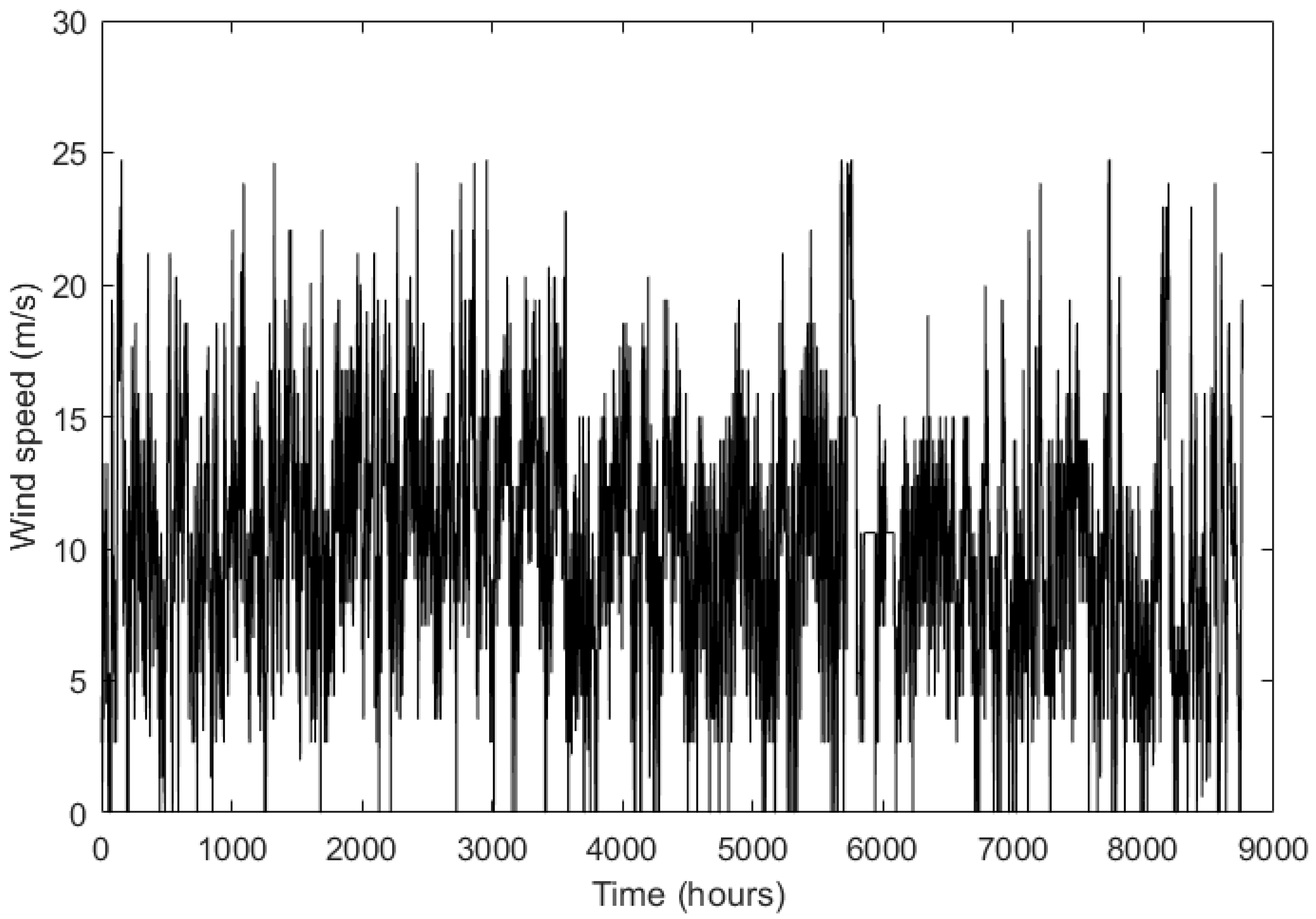
The distribution of wind speed with a range from 0 to 25 m/s for the year 2018 at the Chapman Ranch wind farm is shown in Figure 13. These hourly wind speed values are statistically analyzed to obtain the wind speed series between the successive seconds using Gaussian distribution given by Equation (74). The mean wind speed and the standard deviation used for the Gaussian distribution are 10.38 and three. The wind speed generated using the Gaussian distribution, which is given as disturbance input to the wind turbine model, is shown in Figure 14. The reference model and the compensator model for this case study are the same as the 2 MW and the 5 MW wind turbine plants.

The rotor speed tracking of the wind turbine in the case study is given in Figure 15. The short spikes in the result correspond to the spikes in the wind speed distribution, where the wind speed shifts between the three regions of operation. Similar to the combined case explained in Section 5.3, the adaptive controller design ensures the satisfactory tracking of the rotor speed in all operating regions of the wind turbine.

7. Conclusions

Wind turbine control plays a prominent role in developing wind turbine technology, mainly for pitch control, due to the nonlinear aerodynamics of the rotor at high turbulent wind speeds. This research proposes a robust adaptive control for the complex dynamic system of the wind turbine to design a pitch controller and a torque controller in three operating regions of the wind turbine. For regions one and two, the system is controlled by the adaptive torque control mechanism. For region three, the system output is controlled by an adaptive pitch control algorithm. The proposed control is implemented on 2 MW and 5 MW wind turbines to test its robustness to parameter uncertainty. The results indicate that this adaptive controller can be used for any size of the wind turbine as long as the plant satisfies the ASPR condition. The results also indicate that the rotor speed of the wind turbine is maintained to follow the nominal value in all cases of the simulation. The case study results show that the adaptive controller works efficiently for any kind of uncertainties and always gives a satisfactory tracking of the rotor angular speed.

References

1. Kumar, V.; Pandey, A.S.; Sinha, S.K. Grid integration and power quality issues of wind and solar energy system: A review. In Proceedings of the 2016 International Conference on Emerging Trends in Electrical Electronics & Sustainable Energy Systems (ICETEESES), Sultanpur, India, 11–12 March 2016; pp. 71–80. [Google Scholar]
2. Chamsai, T.; Jirawattana, P.; Radpukdee, T. Robust Adaptive PID controller for a class of uncertain nonlinear systems: An application for speed tracking control of an SI engine. Math. Probl. Eng. 2015, 2015, 1–12. [Google Scholar] [CrossRef]
3. Mattavelli, P.; Rossetto, L.; Spiazzi, G.; Tenti, P. General-purpose fuzzy controller for DC/DC converters. IEEE Trans. Power Electron. 1997. [Google Scholar] [CrossRef] [Green Version]
4. Camblong, H. Digital robust control of a variable speed pitch regulated wind turbine for above rated wind speeds. Control Eng. Pract. 2008, 16, 946–958. [Google Scholar] [CrossRef]
5. Shirazi, F.A.; Grigoriadis, K.M.; Viassolo, D. Wind turbine linear parameter varying control using fast code. In Proceedings of the Volume 2: Legged Locomotion; Mechatronic Systems; Mechatronics; Mechatronics for Aquatic Environments; MEMS Control; Model Predictive Control; Modeling and Model-Based Control of Advanced IC Engines, Fort Lauderdale, FL, USA, 17–19 October 2012; p. 771. [Google Scholar]
6. Ren, Y.; Li, L.; Brindley, J.; Jiang, L. Nonlinear PI control for variable pitch wind turbine. Control Eng. Pract. 2016, 50, 84–94. [Google Scholar] [CrossRef] [Green Version]
7. Schlipf, D.; Schlipf, D.J.; Kühn, M. Nonlinear model predictive control of wind turbines using LIDAR: Nonlinear model predictive control of wind turbines using LIDAR. Wind Energy 2013, 16, 1107–1129. [Google Scholar] [CrossRef]
8. Mullane, A.; Lightbody, G.; Yacamini, R. Adaptive Control of Variable Speed Wind Turbines. Rev. Energ. Ren. Power Eng. 2001, 101–110. [Google Scholar]
9. Kadri, M.B.; Khan, S. Fuzzy adaptive pitch controller of a wind turbine. In Proceedings of the 2012 15th International Multitopic Conference (INMIC), Islamabad, Pakistan, 13–15 December 2012; pp. 105–110. [Google Scholar]
10. Jafarnejadsani, H.; Pieper, J.; Ehlers, J. Adaptive control of a variable-speed variable-pitch wind turbine using radial-basis function neural network. IEEE Trans. Control Syst. Technol. 2013, 21, 2264–2272. [Google Scholar] [CrossRef]
11. Lakshmi, K.V.; Srinivas, P. Fuzzy adaptive PID control of pitch system in variable speed wind turbines. In Proceedings of the 2014 International Conference on Issues and Challenges in Intelligent Computing Techniques (ICICT), Ghaziabad, India, 7–8 February 2014; pp. 52–57. [Google Scholar]
12. Yuan, Y.; Tang, J. Adaptive pitch control of wind turbine for load mitigation under structural uncertainties. Renew. Energy 2017, 105, 483–494. [Google Scholar] [CrossRef] [Green Version]
13. Xiao, Y.; Hong, Y.; Chen, X.; Huo, W. Switching control of wind turbine sub-controllers based on an active disturbance rejection technique. Energies 2016, 9, 793. [Google Scholar] [CrossRef] [Green Version]
14. Garcia-Sanz, M.; Constantine, H. Wind Energy Systems: Control Engineering Design; CRC Press: Boca Raton, FL, USA, 2012. [Google Scholar]
15. Garcia-Sanz, M. Robust Control Engineering: Practical QFT Solutions; CRC Press: Boca Raton, FL, USA, 2017. [Google Scholar]
16. Ozcelik, S.; DeMarchi, J.; Kaufman, H.; Craig, K. Control of an inverted pendulum using direct model reference adaptive control. IFAC Proc. Vol. 1997, 30, 585–590. [Google Scholar] [CrossRef]
17. Aksoy, H.; Fuat Toprak, Z.; Aytek, A.; Erdem Ünal, N. Stochastic generation of hourly mean wind speed data. Renew. Energy 2004, 29, 2111–2131. [Google Scholar] [CrossRef]
18. Hayajneh, H.S.; Bashetty, S.; Salim, M.N.B.; Zhang, X. Techno-economic analysis of a battery energy storage system with combined stationary and mobile applications. In Proceedings of the 2018 IEEE Conference on Technologies for Sustainability (SusTech), Long Beach, CA, USA, 11–13 November 2018; pp. 1–6. [Google Scholar]
19. Zhang, Z.; Basu, B.; Nielsen, S.R.K. Real-time hybrid aeroelastic simulation of wind turbines with various types of full-scale tuned liquid dampers. Wind Energy 2019, 22. [Google Scholar] [CrossRef]
20. Jain, P. Wind Energy Engineering; McGraw-Hill: New York, NY, USA, 2011. [Google Scholar]
Figure 1. Power characteristics for different operating regions of a wind turbine.
Energies 13 01195 g001
Figure 2. Power coefficient ( C P ) vs. tip speed ratio ( λ ) for different pitch angles ( ϕ ).
Energies 13 01195 g002
Figure 3. Adaptive control structure.
Energies 13 01195 g003
Figure 4. Wind turbine adaptive controller block diagram.
Energies 13 01195 g004
Figure 5. Wind speed distribution in region three.
Energies 13 01195 g005
Figure 6. Steady-state rotor speed regulation of the 2 MW and the 5 MW wind turbines in region three.
Energies 13 01195 g006
Figure 7. Pitch angle control input up(t) to the plant and CP in region three.
Energies 13 01195 g007
Figure 8. Wind speed distribution in the torque control region.
Energies 13 01195 g008
Figure 9. Steady-state rotor speed tracking of the 2 MW and the 5 MW wind turbines in the torque control region.
Energies 13 01195 g009
Figure 10. Generator torque control input up(t) to the plant in regions one and two.
Energies 13 01195 g010
Figure 11. Wind speed profile for the wind turbines in combined cases.
Energies 13 01195 g011
Figure 12. Steady-state rotor speed tracking of the 2 MW and the 5 MW wind turbines.
Energies 13 01195 g012
Figure 13. Wind speed distribution at Chapman Ranch wind farm for the year 2018.
Energies 13 01195 g013
Figure 14. Wind speed obtained using Gaussian distribution.
Energies 13 01195 g014
Figure 15. Steady-state rotor speed tracking of the wind turbine in Chapman Ranch.
Energies 13 01195 g015