An Integrated Energy Simulation Model for Buildings


 and
and
Abstract
1. Introduction
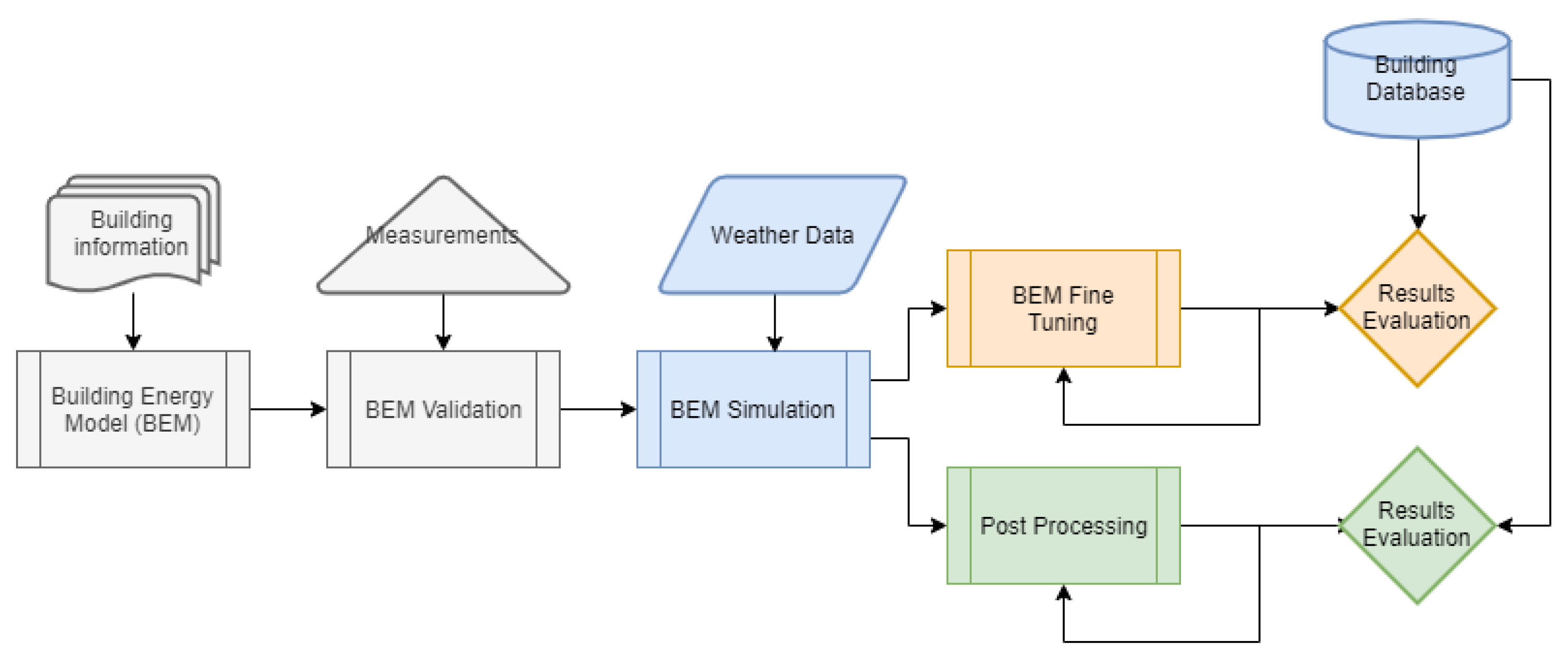
2. Methodology and Modeling Approaches
2.1. The Energy Simulation Model: General Presentation of the Model, Areas of Application, Advantages, and Shortcomings
- is the absorbed direct and diffuse solar (short wavelength) radiation and heat flux
- is the net long wavelength (thermal) radiation flux exchange with the air and surroundings
- is the convective flux exchange with the outside air
- is the conduction heat flux (q/A) into the wall
- is the long-wave emittance of the surface
- is the Stefan–Boltzmann constant
- is the view factor of wall surface to ground surface temperature
- is the view factor of wall surface to sky temperature
- is the view factor of wall surface to air temperature
- is the outside surface temperature
- is the ground surface temperature
- is the sky temperature
- is the air temperature
- is the rate of exterior convective heat transfer
- is the exterior convection coefficient
- A is the surface area
- is the surface temperature
- is the outdoor air temperature
- is the conductive heat flux for the current time step
- T is temperature
- i indicates the internal element of the building
- o indicates the external element of the building
- X,Y are the response factors
- is the outside CTF coefficient, j = 0,1,...nz
- is the cross CTF coefficient, j = 0,1,...nz
- is the inside CTF coefficient, j = 0,1,...nz
- is the flux CTF coefficient, j = 0,1,...nq
- is the inside surface temperature
- is the outside surface temperature
- is the conduction heat flux on the outside face
- is the conduction heat flux on the inside face
- is the sum of convective heat transfer from the zone surfaces
- is the convective heat transfer from the zone surfaces
- is the heat transfer due to infiltration of outside air
- is the heat transfer due to interzone air mixing
- is the air systems output
- is the energy stored in zone air, and
- is the user defined infiltration value (ACH)
- is the zone air temperature at current conditions (deg C)
- is the outdoor air dry-bulb temperature (deg C)
- is a user defined schedule value between 0 and 1
- A is the constant term coefficient
- B is the temperature term coefficient
- C is the velocity term coefficient
- D is the velocity squared coefficient
- is the user defined ventilation value (ACH)
- is the zone air temperature at current conditions (deg C)
- is the outdoor air dry-bulb temperature (deg C)
- is a user defined schedule value between 0 and 1
- A is the constant term coefficient
- B is the temperature term coefficient
- C is the velocity term coefficient
- D is the velocity squared coefficient
2.2. Shape Modeling and Systematic Inefficiencies Correction of the Prediction Model: Presentation of the Properties and Capabilities of the Shape Invariant Model and Implementation in the Current Study
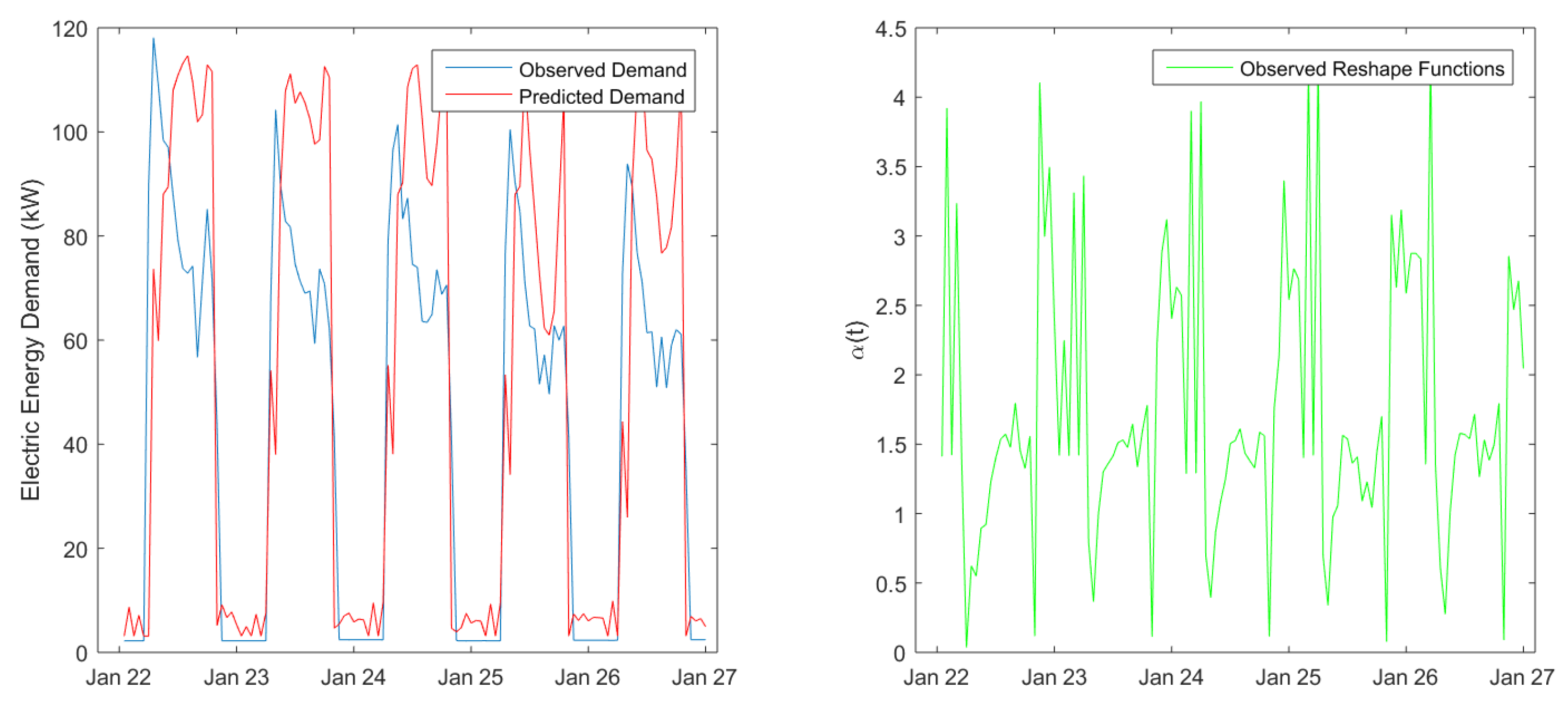
2.2.1. The Shape Model Approach
2.2.2. The Weighted Shape Model Approach
2.3. Postprocessing Using Kalman Filtering: The General Algorithm, Capabilities and Areas of Application, and the Filter Proposed for the Present Work
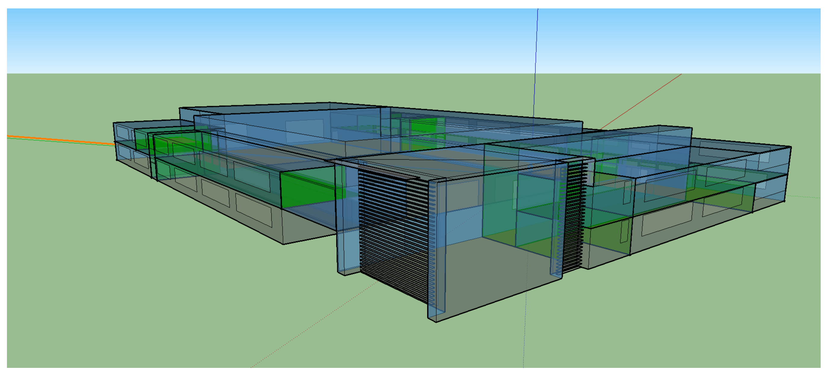
3. Test Cases and Results
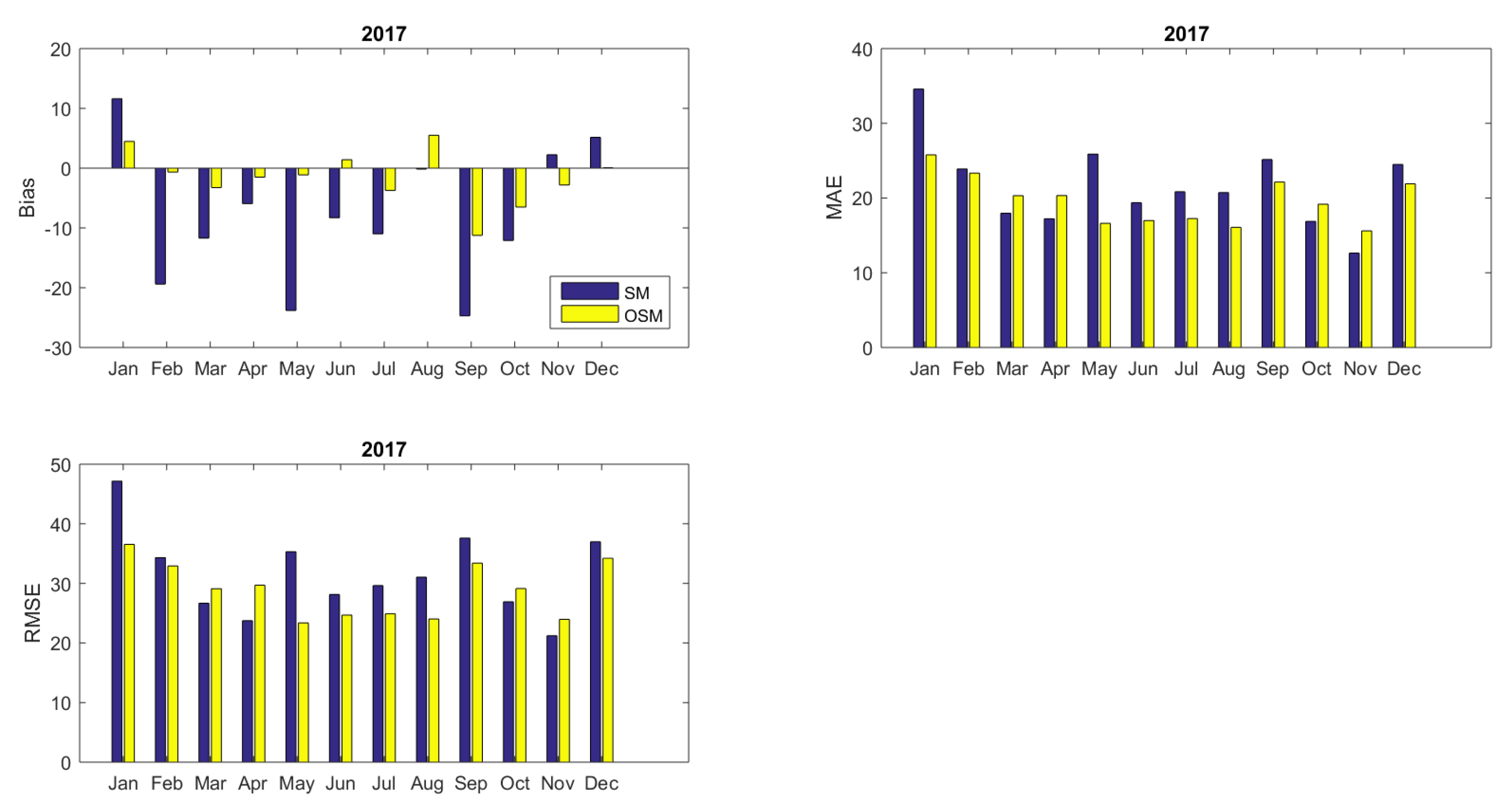
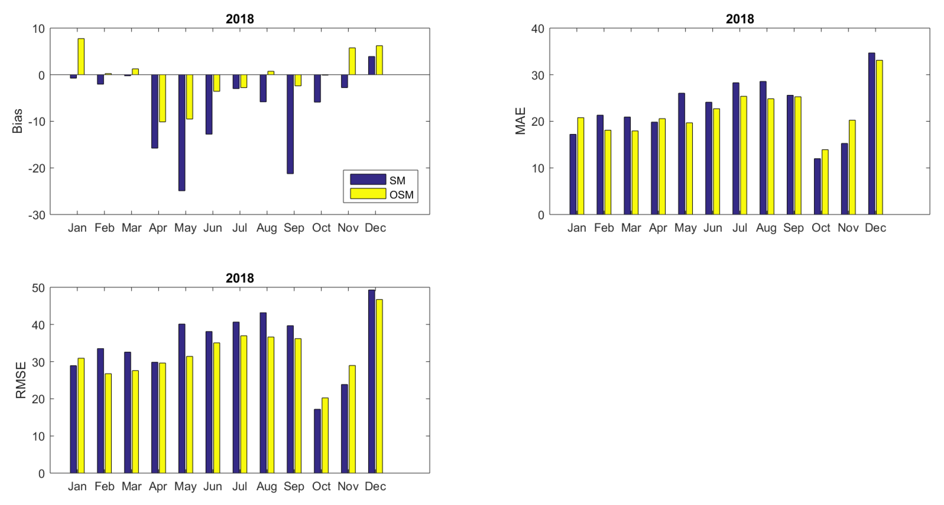
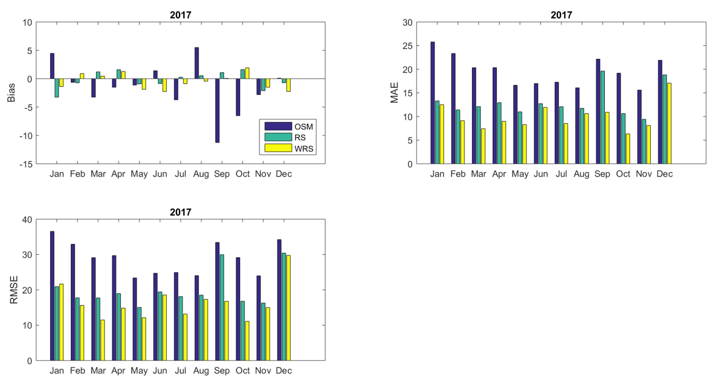
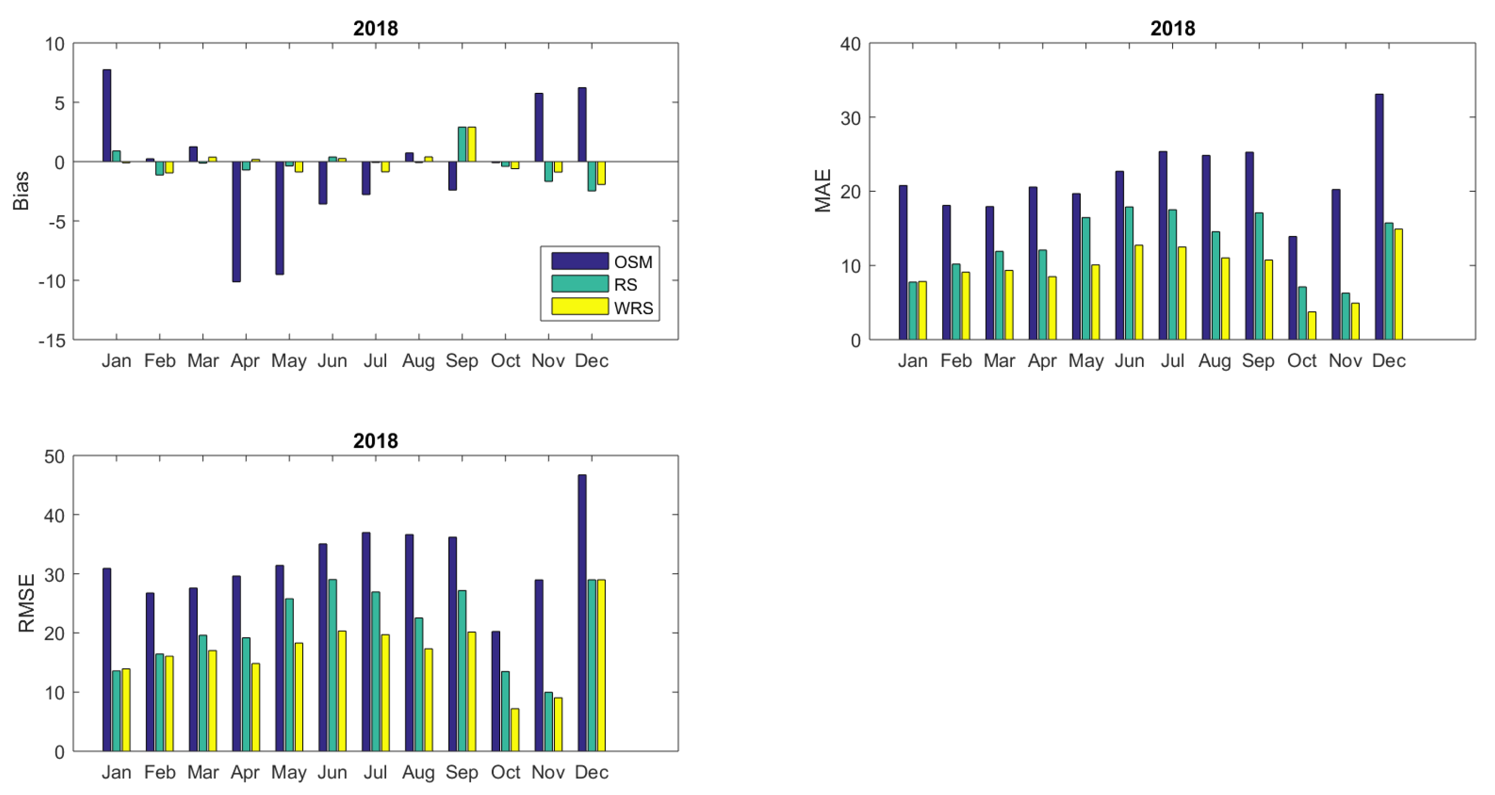
- Prediction Bias, , indicating any systematic underestimation or overestimation of the quantity of interest.
- Mean Absolute Error, , indicating the mean absolute deviance of the model predictions from the true value.
- Root Mean Squared Error, , indicating the mean squared deviance of the model predictions from the true value.
- Nash–Sutcliffe model efficiency coefficient, which is used to assess the predictive power of the model:taking values on where an index equal to zero corresponds to a perfect prediction whereas values below zero corresponds to the case where the prediction model was outperformed by a reference model .
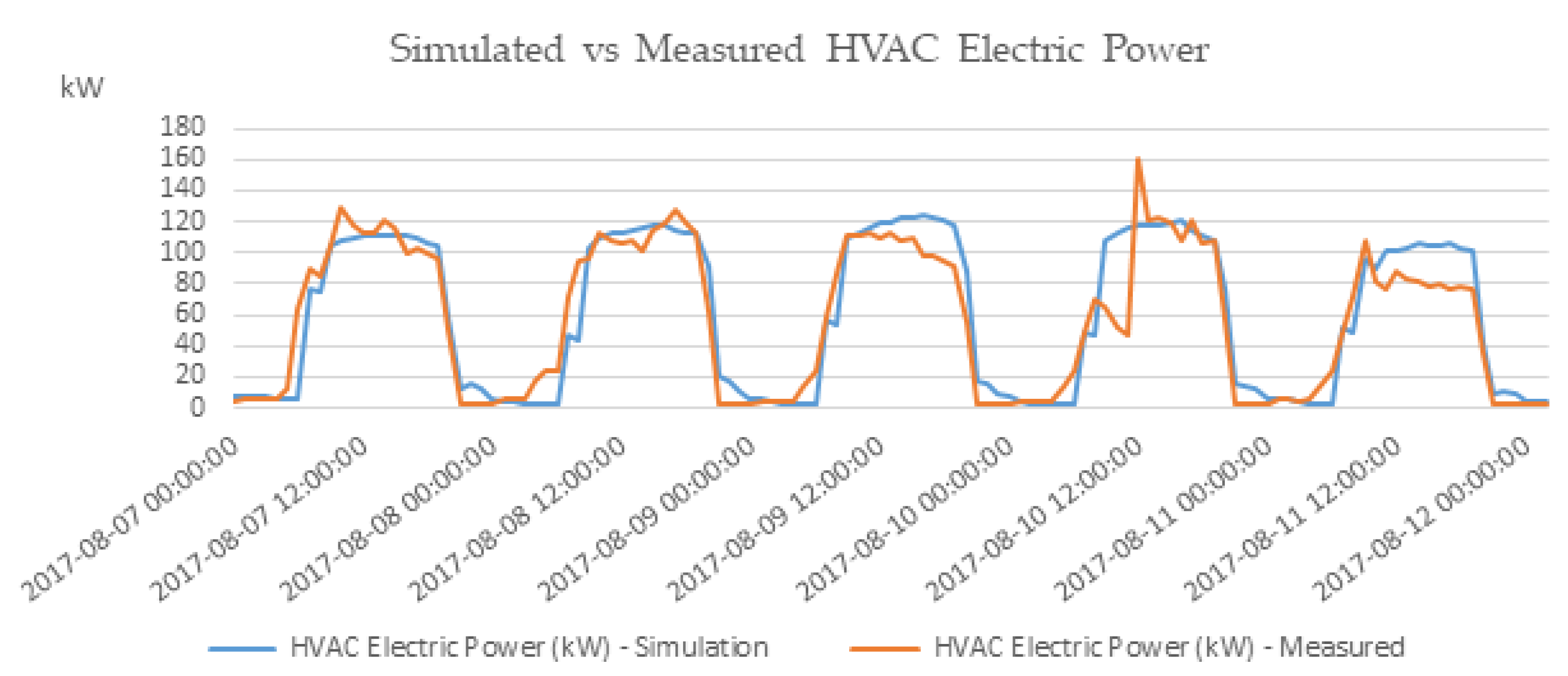
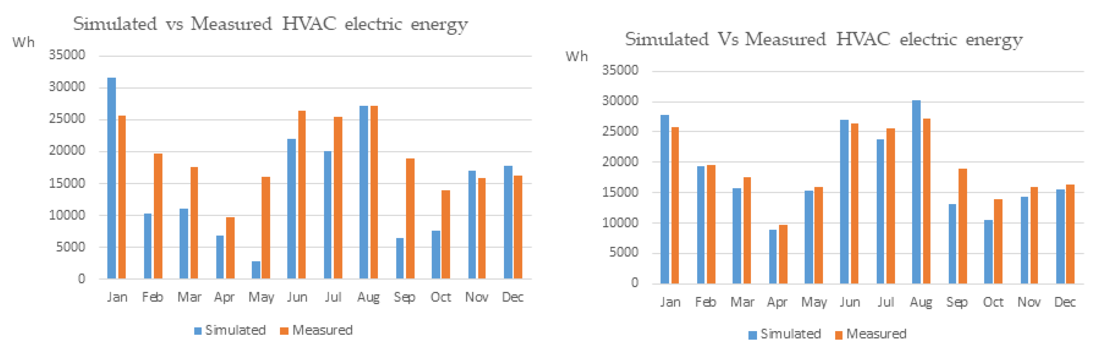
3.1. Indicative Analysis of the Initial Simulation Results: Revealing the Weak Points
3.2. Diagnostic Results for the Complete Model Outputs
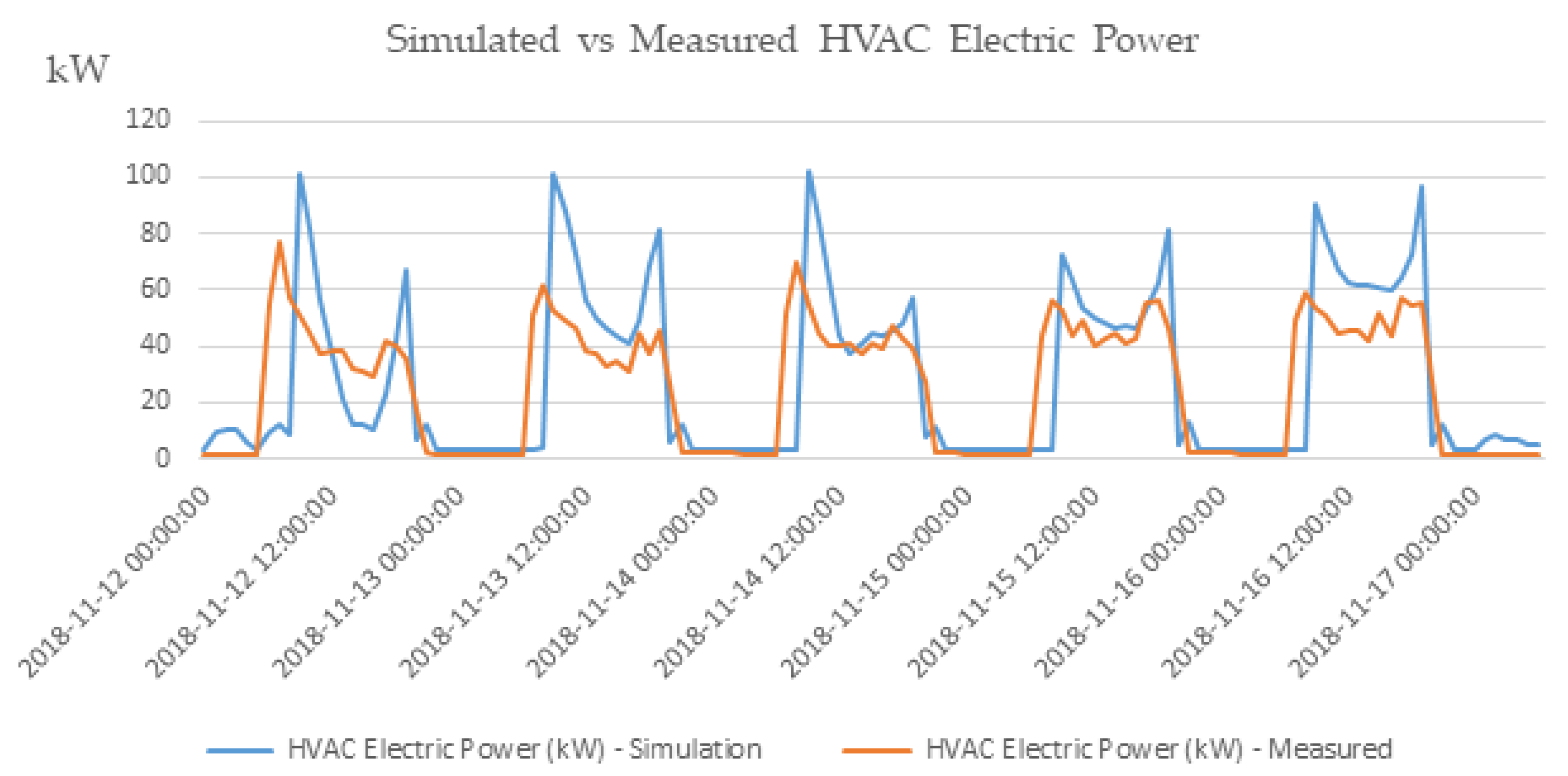
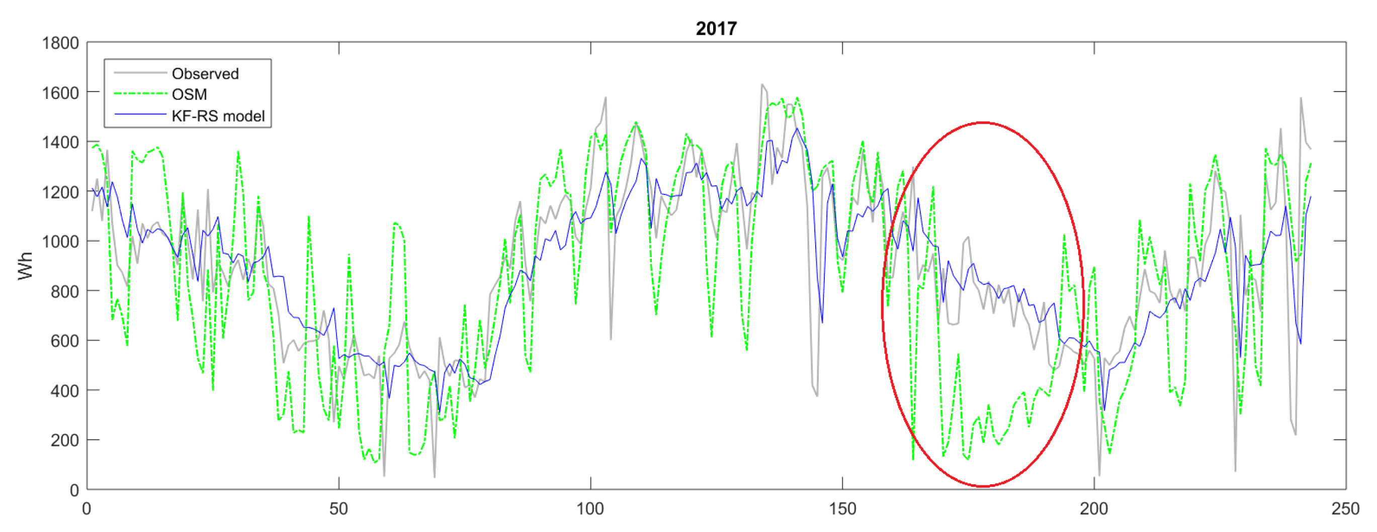
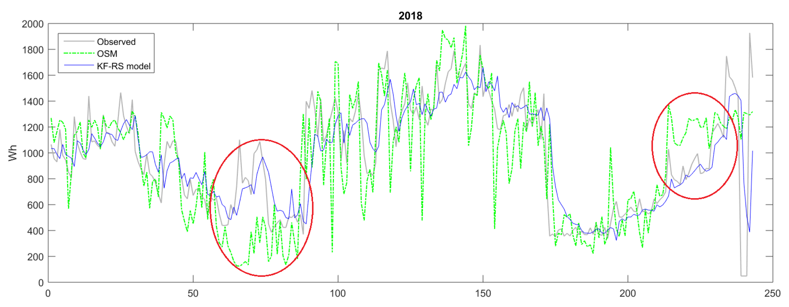
3.2.1. Evaluating Intra-Day Energy Demand Predictions
3.2.2. Evaluating Daily Summaries Energy Demand Predictions
4. Conclusions
Author Contributions
Funding
Conflicts of Interest
References
- International Energy Agency. Available online: https://www.iea.org/topics/energy-efficiency/buildings/ (accessed on 18 September 2019).
- Athienitis, A.K.; O’Brien, W. Modeling, Design, and Optimization of Net-Zero Energy Buildings; Wiley Online Library: Hoboken, NJ, USA, 2015. [Google Scholar]
- Zhao, H.x.; Magoulès, F. A review on the prediction of building energy consumption. Renew. Sustain. Energy Rev. 2012, 16, 3586–3592. [Google Scholar] [CrossRef]
- Santamouris, M. Advances in Building Energy Research; Taylor & Francis: Hoboken, NJ, USA, 2010; Volume 4. [Google Scholar]
- Foucquier, A.; Robert, S.; Suard, F.; Stéphan, L.; Jay, A. State of the art in building modeling and energy performances prediction: A review. Renew. Sustain. Energy Rev. 2013, 23, 272–288. [Google Scholar] [CrossRef]
- SPARK 2.0 REFERENCE MANUAL Simulation Problem Analysis and Research Kernel. Available online: https://simulationresearch.lbl.gov/VS201/doc/SPARKreferenceManual.pdf (accessed on 11 November 2019).
- Harish, V.; Kumar, A. A review on modeling and simulation of building energy systems. Renew. Sustain. Energy Rev. 2016, 56, 1272–1292. [Google Scholar] [CrossRef]
- Naji, S.; Keivani, A.; Shamshirband, S.; Alengaram, U.J.; Jumaat, M.Z.; Mansor, Z.; Lee, M. Estimating building energy consumption using extreme learning machine method. Energy 2016, 97, 506–516. [Google Scholar] [CrossRef]
- Robinson, C.; Dilkina, B.; Hubbs, J.; Zhang, W.; Guhathakurta, S.; Brown, M.A.; Pendyala, R.M. Machine learning approaches for estimating commercial building energy consumption. Appl. Energy 2017, 208, 889–904. [Google Scholar] [CrossRef]
- Amasyali, K.; El-Gohary, N.M. A review of data-driven building energy consumption prediction studies. Renew. Sustain. Energy Rev. 2018, 81, 1192–1205. [Google Scholar] [CrossRef]
- Wei, Y.; Zhang, X.; Shi, Y.; Xia, L.; Pan, S.; Wu, J.; Han, M.; Zhao, X. A review of data-driven approaches for prediction and classification of building energy consumption. Renew. Sustain. Energy Rev. 2018, 82, 1027–1047. [Google Scholar] [CrossRef]
- De Wit, S.; Augenbroe, G. Analysis of uncertainty in building design evaluations and its implications. Energy Build. 2002, 34, 951–958. [Google Scholar] [CrossRef]
- Ryan, E.M.; Sanquist, T.F. Validation of building energy modeling tools under idealized and realistic conditions. Energy Build. 2012, 47, 375–382. [Google Scholar] [CrossRef]
- Maile, T.; Bazjanac, V.; Fischer, M. A method to compare simulated and measured data to assess building energy performance. Build. Environ. 2012, 56, 241–251. [Google Scholar] [CrossRef]
- Coakley, D.; Raftery, P.; Keane, M. A review of methods to match building energy simulation models to measured data. Renew. Sustain. Energy Rev. 2014, 37, 123–141. [Google Scholar] [CrossRef]
- M & V Guidelines: Measurement and Verification for Performance-Based Contracts Version 4.0. Available online: https://www.energy.gov/sites/prod/files/2016/01/f28/mv_guide_4_0.pdf (accessed on 12 August 2019).
- Royapoor, M.; Roskilly, T. Building model calibration using energy and environmental data. Energy Build. 2015, 94, 109–120. [Google Scholar] [CrossRef]
- O’Neill, Z.D.; Bailey, T.G.; Eisenhower, B.A.; Fonoberov, V.A. Calibration of a building energy model considering parametric uncertainty. ASHRAE Trans. 2012, 118, 189–196. [Google Scholar]
- O’Neill, Z.D.; Eisenhower, B.A.; Bailey, T.G.; Narayanan, S.; Fonoberov, V.A. Modeling and calibration of energy models for a DoD building. ASHRAE Trans. 2011, 117, 358–365. [Google Scholar]
- EnergyPlusTM, Engineering Reference Documentation Version 9.1.0, National Renewable Energy Laboratory. 2019. Available online: https://energyplus.net (accessed on 12 August 2019).
- Brackney, L.; Parker, A.; Macumber, D.; Benne, K. Building Energy Modeling with OpenStudio; Springer: Berlin, Germany, 2018. [Google Scholar]
- Wand, M.P.; Jones, M.C. Kernel Smoothing; Chapman and Hall/CRC: Boca Raton, FL, USA, 1994. [Google Scholar]
- Ramsay, J.O.; Silverman, B.W. Applied Functional Data Analysis: Methods and Case Studies; Springer: New York, NY, USA, 2007. [Google Scholar]
- Gu, C. Smoothing Spline ANOVA Models; Springer Science & Business Media: Berlin, Germany, 2013; Volume 297. [Google Scholar]
- Lawton, W.; Sylvestre, E.; Maggio, M. Self modeling nonlinear regression. Technometrics 1972, 14, 513–532. [Google Scholar] [CrossRef]
- Kneip, A.; Engel, J. Model estimation in nonlinear regression under shape invariance. Annals Stat. 1995, 23, 551–570. [Google Scholar] [CrossRef]
- Gervini, D.; Gasser, T. Self-modeling warping functions. J. R. Stat. Soc. Ser. B (Statistical Methodol.) 2004, 66, 959–971. [Google Scholar] [CrossRef]
- Papayiannis, G.I.; Giakoumakis, E.A.; Manios, E.D.; Moulopoulos, S.D.; Stamatelopoulos, K.S.; Toumanidis, S.T.; Zakopoulos, N.A.; Yannacopoulos, A.N. A functional supervised learning approach to the study of blood pressure data. Stat. Med. 2018, 37, 1359–1375. [Google Scholar] [CrossRef]
- Fréchet, M. Les éléments aléatoires de nature quelconque dans un espace distancié. Ann. De L’institut Henri Poincaré 1948, 10, 215–310. [Google Scholar]
- Izem, R.; Marron, J.S. Analysis of nonlinear modes of variation for functional data. Electron. J. Stat. 2007, 1, 641–676. [Google Scholar] [CrossRef]
- Bigot, J.; Charlier, B. On the consistency of Fréchet means in deformable models for curve and image analysis. Electron. J. Stat. 2011, 5, 1054–1089. [Google Scholar] [CrossRef]
- Kalman, R.E. A new approach to linear filtering and prediction problems. J. Basic Eng. 1960, 82, 34–45. [Google Scholar] [CrossRef]
- Kalman, R.E.; Bucy, R.S. New results in linear filtering and prediction theory. J. Basic Eng. 1961, 83, 95–108. [Google Scholar] [CrossRef]
- Kalnay, E. Atmospheric Modeling, Data Assimilation and Predictability; Cambridge University Press: Cambridge, UK, 2003. [Google Scholar]
- Crochet, P. Adaptive Kalman filtering of 2-metre temperature and 10-metre wind-speed forecasts in Iceland. Meteorol. Appl. 2004, 11, 173–187. [Google Scholar] [CrossRef]
- Galanis, G.; Anadranistakis, M. A one-dimensional Kalman filter for the correction of near surface temperature forecasts. Meteorol. Appl. 2002, 9, 437–441. [Google Scholar] [CrossRef]
- Emmanouil, G.; Galanis, G.; Kallos, G. Statistical methods for the prediction of night-time cooling and minimum temperature. Meteorol. Appl. 2006, 13, 169–178. [Google Scholar] [CrossRef][Green Version]
- Galanis, G.; Louka, P.; Katsafados, P.; Pytharoulis, I.; Kallos, G. Applications of Kalman filters based on non-linear functions to numerical weather predictions. Ann. Geophys. 2006, 24, 2451–2460. [Google Scholar] [CrossRef]
- Hua, S.; Wang, S.; Jin, S.; Feng, S.; Wang, B. Wind speed optimisation method of numerical prediction for wind farm based on Kalman filter method. J. Eng. 2017, 2017, 1146–1149. [Google Scholar] [CrossRef]
- Emmanouil, G.; Galanis, G.; Kallos, G. Combination of statistical Kalman filters and data assimilation for improving ocean waves analysis and forecasting. Ocean Model. 2012, 59, 11–23. [Google Scholar] [CrossRef]
- Galanis, G.; Emmanouil, G.; Chu, P.C.; Kallos, G. A new methodology for the extension of the impact of data assimilation on ocean wave prediction. Ocean Dyn. 2009, 59, 523–535. [Google Scholar] [CrossRef]
- Galanis, G.; Chu, P.C.; Kallos, G. Statistical post processes for the improvement of the results of numerical wave prediction models. A combination of Kolmogorov-Zurbenko and Kalman filters. J. Oper. Oceanogr. 2011, 4, 23–31. [Google Scholar] [CrossRef][Green Version]
- Patlakas, P.; Drakaki, E.; Galanis, G.; Spyrou, C.; Kallos, G. Wind gust estimation by combining a numerical weather prediction model and statistical postprocessing. Energy Procedia 2017, 125, 190–198. [Google Scholar] [CrossRef]
- Samalot, A.; Astitha, M.; Yang, J.; Galanis, G. Combined kalman filter and universal kriging to improve storm wind speed predictions for the northeastern United States. Weather Forecast. 2019, 34, 587–601. [Google Scholar] [CrossRef]
- Louka, P.; Galanis, G.; Siebert, N.; Kariniotakis, G.; Katsafados, P.; Pytharoulis, I.; Kallos, G. Improvements in wind speed forecasts for wind power prediction purposes using Kalman filtering. J. Wind Eng. Ind. Aerodyn. 2008, 96, 2348–2362. [Google Scholar] [CrossRef]
- Pelland, S.; Galanis, G.; Kallos, G. Solar and photovoltaic forecasting through postprocessing of the Global Environmental Multiscale numerical weather prediction model. Prog. Photovoltaics: Res. Appl. 2013, 21, 284–296. [Google Scholar] [CrossRef]
- Stathopoulos, C.; Kaperoni, A.; Galanis, G.; Kallos, G. Wind power prediction based on numerical and statistical models. J. Wind Eng. Ind. Aerodyn. 2013, 112, 25–38. [Google Scholar] [CrossRef]
- MyLeaf Platform - Loccioni Group. Available online: https://https://myleaf2.loccioni.com (accessed on 26 July 2018).
- Provata, E.; Kolokotsa, D.; Papantoniou, S.; Pietrini, M.; Giovannelli, A.; Romiti, G. Development of optimization algorithms for the Leaf Community microgrid. Renew. Energy 2015, 74, 782–795. [Google Scholar] [CrossRef]
- Kampelis, N.; Gobakis, K.; Vagias, V.; Kolokotsa, D.; Standardi, L.; Isidori, D.; Cristalli, C.; Montagnino, F.; Paredes, F.; Muratore, P.; et al. Evaluation of the performance gap in industrial, residential & tertiary near-Zero energy buildings. Energy Build. 2017, 148, 58–73. [Google Scholar]


| 2017 | Simulated - Baseline Model (MWh) | Simulated - Optimized Model (MWh) | Measured (MWh) |
|---|---|---|---|
| Jan | 31.55 | 27.79 | 25.72 |
| Feb | 10.26 | 19.27 | 19.61 |
| Mar | 11.09 | 15.76 | 17.55 |
| Apr | 6.79 | 8.92 | 9.64 |
| May | 2.90 | 15.40 | 16.02 |
| Jun | 21.97 | 27.10 | 26.34 |
| Jul | 20.02 | 23.69 | 25.55 |
| Aug | 27.19 | 30.31 | 27.27 |
| Sep | 6.39 | 13.15 | 18.87 |
| Oct | 7.62 | 10.56 | 14.00 |
| Nov | 17.05 | 14.38 | 15.86 |
| Dec | 17.70 | 15.62 | 16.24 |
| 2018 | Simulated - Baseline Model (MWh) | Simulated - Optimized Model (MWh) | Measured (MWh) |
|---|---|---|---|
| Jan | 22.60 | 27.29 | 23.02 |
| Feb | 21.42 | 22.52 | 22.49 |
| Mar | 20.29 | 21.07 | 20.40 |
| Apr | 5.92 | 8.76 | 13.85 |
| May | 3.27 | 11.76 | 17.01 |
| Jun | 17.65 | 22.30 | 24.09 |
| Jul | 29.32 | 29.45 | 30.90 |
| Aug | 30.94 | 34.56 | 34.16 |
| Sep | 9.92 | 18.99 | 20.13 |
| Oct | 6.88 | 10.06 | 10.11 |
| Nov | 14.29 | 18.80 | 15.75 |
| Dec | 17.96 | 18.46 | 18.14 |
| Model | Bias | MAE | RMSE | NSE | Bias | MAE | RMSE | NSE |
|---|---|---|---|---|---|---|---|---|
| 2017 | 2018 | |||||||
| SM | −8.67 | 21.32 | 31.66 | 0.00 | −7.67 | 22.66 | 35.56 | 0.00 |
| OSM | −1.79 | 19.39 | 28.80 | 0.17 | −0.63 | 21.77 | 32.58 | 0.16 |
| RS | −0.14 | 12.92 | 20.46 | 0.58 | −0.25 | 12.91 | 22.01 | 0.62 |
| w−RS | −0.51 | 9.91 | 17.03 | 0.71 | −0.18 | 9.58 | 17.65 | 0.75 |
| KF−RS | 0.20 | 11.33 | 17.60 | 0.70 | −0.36 | 12.67 | 18.73 | 0.73 |
| Model | Bias | MAE | RMSE | NSE | Bias | MAE | RMSE | NSE |
|---|---|---|---|---|---|---|---|---|
| 2017 | 2018 | |||||||
| SM | −195.00 | 344.65 | 423.71 | 0.00 | −182.59 | 306.54 | 413.80 | 0.00 |
| OSM | −37.54 | 237.38 | 304.32 | 0.30 | −12.80 | 232.49 | 328.62 | 0.30 |
| RS | −1.90 | 192.54 | 272.03 | 0.44 | −6.09 | 194.10 | 295.32 | 0.32 |
| w−RS | −11.18 | 144.97 | 226.93 | 0.61 | −4.39 | 139.18 | 238.78 | 0.50 |
| KF−RS | −0.73 | 143.46 | 207.51 | 0.66 | −1.70 | 155.74 | 247.69 | 0.51 |
© 2020 by the authors. Licensee MDPI, Basel, Switzerland. This article is an open access article distributed under the terms and conditions of the Creative Commons Attribution (CC BY) license (http://creativecommons.org/licenses/by/4.0/).
Share and Cite
Kampelis, N.; Papayiannis, G.I.; Kolokotsa, D.; Galanis, G.N.; Isidori, D.; Cristalli, C.; Yannacopoulos, A.N. An Integrated Energy Simulation Model for Buildings. Energies 2020, 13, 1170. https://doi.org/10.3390/en13051170
Kampelis N, Papayiannis GI, Kolokotsa D, Galanis GN, Isidori D, Cristalli C, Yannacopoulos AN. An Integrated Energy Simulation Model for Buildings. Energies. 2020; 13(5):1170. https://doi.org/10.3390/en13051170
Chicago/Turabian StyleKampelis, Nikolaos, Georgios I. Papayiannis, Dionysia Kolokotsa, Georgios N. Galanis, Daniela Isidori, Cristina Cristalli, and Athanasios N. Yannacopoulos. 2020. "An Integrated Energy Simulation Model for Buildings" Energies 13, no. 5: 1170. https://doi.org/10.3390/en13051170
APA StyleKampelis, N., Papayiannis, G. I., Kolokotsa, D., Galanis, G. N., Isidori, D., Cristalli, C., & Yannacopoulos, A. N. (2020). An Integrated Energy Simulation Model for Buildings. Energies, 13(5), 1170. https://doi.org/10.3390/en13051170