Abstract
The operation of buildings is linked to approximately 36% of the global energy consumption, 40% of greenhouse gas emissions, and climate change. Assessing the energy consumption and efficiency of buildings is a complex task addressed by a variety of methods. Building energy modeling is among the dominant methodologies in evaluating the energy efficiency of buildings commonly applied for evaluating design and renovation energy efficiency measures. Although building energy modeling is a valuable tool, it is rarely the case that simulation results are assessed against the building’s actual energy performance. In this context, the simulation results of the HVAC energy consumption in the case of a smart industrial near-zero energy building are used to explore areas of uncertainty and deviation of the building energy model against measured data. Initial model results are improved based on a trial and error approach to minimize deviation based on key identified parameters. In addition, a novel approach based on functional shape modeling and Kalman filtering is developed and applied to further minimize systematic discrepancies. Results indicate a significant initial performance gap between the initial model and the actual energy consumption. The efficiency and the effectiveness of the developed integrated model is highlighted.
1. Introduction
Energy consumption in the building sector (combined with buildings construction) is associated with 36% of global final energy consumption and approximately 40% of total direct and indirect CO emissions. Associated figures rise every year mainly due to (a) improved energy access levels in developing countries, (b) increased ownership levels of energy consuming devices, and (c) the growth of global buildings floor area [1]. Measures to reduce energy consumption at building level include passive and active energy efficiency measures, storage, energy management, and building integrated renewable energy systems (e.g., solar, geothermal, and wind). Design and modeling of integrated energy systems in net zero energy buildings is discussed by Athienitis and O’Brien [2].
Assessing energy efficiency in buildings is a complex task which varies according to the aim of the analysis and the specificity of each case. In any case, expert knowledge and a set of technical and non-technical information is required. Technical information usually concerns the geometry and thermal characteristics of the building envelope, the design and operation of HVAC system, as well as data from measurements regarding indoor/outdoor climate conditions and energy end usage. Non-technical data in some cases are associated with occupancy levels, clothing levels, users behavior, perceptions, personal economics, and preferences.
Several decades now, significant research efforts have been directed towards evaluating energy efficiency in buildings. Research results have been applied in advancing state-of-the-art, knowledge and understanding, fostering new policies, better regulation, and innovations. In this context, several methods have been developed and evolved along with the creation of custom software applications built to match the needs of certain research and development fields. Various new techniques have been developed and applied to include the physical or “white box” approach, the statistical or machine learning “black box” and the hybrid “gray box” approach. A comparison of the models and applications for predicting building energy consumption in terms of complexity, easiness to use, running speed, input requirements, and accuracy is conducted by Zhao and Magoulès [3].
Physical models are developed to evaluate energy consumption in buildings by using equations of heat and mass transfer between the building and the surrounding environment as well as energy conservation among the building spaces and system components. Such physical models are classified based on the deployed approach and whether it is defined as single (well-mixed) zone [4], multi-zone, or zonal as provided in the state-of-the-art building modeling and energy prediction review by Foucquier et al. [5]. The zonal method is a simplification of CFD in the sense that the thermal zone is divided into several cells and in some cases representation in 2D is feasible. The advantage of the zonal approach is linked to the capability of dealing with large volumes in moderate computation time. SPARK [6] is such an example of a zonal approach software application. According to the multi-zone approach, each one zone or building element (e.g., wall and window) or system (e.g., HVAC system) or specific load (e.g., due to occupancy) is considered as one node for which the heat transfer equations are calculated. Each thermal zone is considered as homogeneous and represented by uniform state variables such as temperature, pressure, relative humidity, etc. The multi-zone or nodal approach is particularly effective when evaluating the energy performance of a building with many thermal zones since computational time for a year round simulation is relatively small. Therefore, the multi-zone approach is suitable for testing the impact of alternative energy efficiency measures provided that a reliable validated model has been created. The main disadvantage of this approach is related to the difficulty in creating a valid building model especially in the absence of holistic information of the building as built, systems installed, operational aspects, and data from measurements. EnergyPlus, ESP-r, and TrnSys are among the most robust and frequently used multi-zone software programs. Benchmarking between building energy simulation software programs reported in the literature is available by Harish et al. [7].
Data-driven methods on the other hand require no physical information, i.e., thermal or geometrical parameters, as they do not deploy heat transfer equations. Regression, Artificial Neural Network (ANN), Genetic Algorithm (GA), and Support Vector Machine (SVM) are some of the techniques used in building energy forecasting based solely on measurements of parameters such as temperature, relative humidity, solar radiation, wind velocity, and energy consumption/production. Machine learning techniques for estimating building energy consumption are exploited by Naji et al. [8] and by Robinson et al. [9]. The main drawback of data-driven methods concerns the interpretation of results in physical terms. Data-driven methods for building energy prediction and classification studies are reviewed by Amasyali and El-Gohary [10] and by Wei et al [11]. Hybrid or “gray box” methods combine physical modeling with data-driven techniques to counterbalance the weaknesses of the “white” and “black” box approaches. Machine learning techniques can be used for parameter estimation, e.g., by coupling a multi-zone model with GA. Another hybrid approach is to use statistical models to improve the performance of physical models with respect to end-uses, which are often unknown and hard to be modeled in a deterministic way.
In contrast with data-driven methods, detailed simulation models do not require conditions monitoring to predict the building performance. However, various sources of uncertainty can lead to significant discrepancies between model predictions and metered energy use. Such sources of uncertainty can be distinguished to specification-related, modeling-related, and scenario-related as discussed by De Wit and Augenbroe [12]. Furthermore, embedding realistic occupant behavior on building modeling and its impact on energy predictions is investigated and addressed as a significant and complex problem by Ryan and Sanquist [13]. Overall, performance gaps can be attributed to a variety of discrepancies in building modeling. A methodology to identify building energy performance problems related to operational, measurements, or simulation aspects is proposed by Maile et al. [14].
Essentially, validation is a critical step to assess the simulation model’s plausibility and reliability. This is especially important for the investigation of energy efficiency measures and the assessment of the actual (not the relative) potential impact in terms of energy and cost savings, environmental performance, thermal comfort, etc. Methods for model validation (otherwise referred to as calibration) are reviewed by Coakley et al. [15], and indicators used in relevant standards (ASHRAE Guideline 14, IPMVP, FEMP) to address acceptance thresholds are discussed [16] by Royapoor and Roskilly [17]. Calibration of a building energy model based on actual measurements is extensively investigated by O’Neil et al. [18]. The building under study hosts offices and conferences rooms, and the authors perform an extensive sensitivity analysis including more than 2000 parameters automatically refined using analytic meta-model-based optimization. A similar approach is followed by O’Neil et al. [19] incorporating EnergyPlus and TRNSYS in their investigation and over 1000 parameters for model calibration.
This paper investigates (i) the validation of a Near-Zero Energy Building (NZEB) simulation model through trial and error approach of important model parameters and (ii) a novel postprocessing approach is proposed which improves the simulation model’s accuracy, combining techniques of functional statistics through appropriate energy shape modeling (employing the concept of deformable models) and Kalman filtering to reduce the remaining biases. Initially, a physical model of the Leaf Lab industrial NZEB in Italy is used to conduct a simulation of the building’s energy consumption for two consecutive years using weather data recorded from onsite meteorological stations. HVAC electric consumption obtained from the simulation is compared to actual measured values to establish the initial (baseline) performance gap. Subsequently, through a trial and error approach, important model parameters are identified and fine-tuned until an improved acceptable correlation between simulated and recorded HVAC electric energy consumption is reached. At a second stage, inconsistencies in the shape of the optimized energy prediction are corrected through an appropriate functional shape/reshape modeling task by comparing recent measured energy demand outputs to predictions and appropriately estimating expected deviations which are used to improve the shape model’s output. At the last step, Kalman filtering is incorporated to remove remaining systematic biases where is needed. Therefore, the original physical model’s results are passed through this integrated model where meaningful interventions are performed to better predict the true situation without neglecting the physical interpretation of the model output. The benefits from the proposed approach are illustrated in the later section (Section 3) with substantial reduction in the error magnitude.
2. Methodology and Modeling Approaches
In this section, we describe the modeling approaches that are used throughout the paper for the prediction of the energy demand. In particular we present (a) the initial energy simulation model and its optimized version by appropriate parameter tuning, (b) the shape model approach in which the optimized output of the energy simulation model is reshaped to further reduce systematic inefficiencies related to discrepancies from the actual shape of the energy demand, and (c) postprocessing using Kalman filtering which reduces remaining systematic errors not captured by the shape model approach. A flowchart of the methodology is presented in Figure 1.
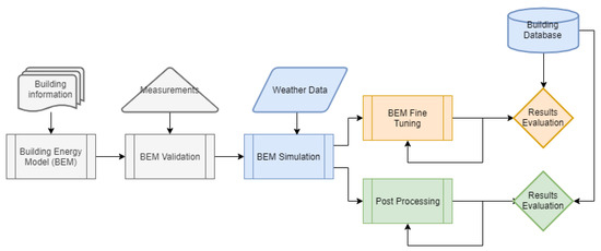
Figure 1.
Flowchart of the high level methodology followed.
2.1. The Energy Simulation Model: General Presentation of the Model, Areas of Application, Advantages, and Shortcomings
EnergyPlus is the simulation engine software used to conduct an integrated simulation of the building, system, and plant whereby supply and demand are matched based on successive iteration substitution following Gauss–Seidel updating [20]. Open Studio is used as the API software for developing and parameterizing the model following the principles outlined by Brackney et al. [21]. Ambient temperature, relative humidity, solar radiation, and wind speed data for 2017 and 2018 was obtained from local meteorological equipment and converted to two yearly weather files. Data of total HVAC energy consumption, for the years 2017 and 2018, are exploited for providing the baseline against which model based results are evaluated.
The simulation model contains, on the one hand, the geometry, construction components and materials of the building under study. For opaque material thickness (m), thermal conductivity (W/mK), density (kg/m), and thermal absorptance properties are edited. For transparent materials, such as glass in windows and sky windows thickness (m), thermal conductivity (W/mK) and optical properties, such as solar, visible, and infrared transmittance, are inserted. On the other hand, a model of the HVAC system is designed based on the installed technologies and adjusted accordingly to the actual key performance heat pump technical parameters such as Coefficients of Performance (COP), fan maximum flow power (m/s), pressure rise, and efficiency. Other parameters such as rated total heating/cooling capacity, and rated and maximum air flow rated are automatically sized based on the software’s calculations. Furthermore, with respect to the operation of the major installed systems, the simulation model takes into account the temperature set points of the HVAC system, ventilation, and infiltration rates (ACH) and a number of schedules to determine artificial lighting, electric equipment, and occupancy. Moreover, humidity control is exercised using appropriate schedules controlling the operation of the HVAC to ensure that the relative humidity during working hours in the various thermal zones varies between 40% and 60%. Subsequently, an intensive search of the parameters that affected the daily, monthly, and annual power distribution profiles is followed to improve the initial results of the model based by minimizing deviation from HVAC power consumption data. Through the trial and error various combinations and fine-tuning of the all of the above parameters is carried out to reach the optimum results when assessing intra-day, monthly, and annual deviation levels.
EnergyPlus simulation is based on heat balance calculations solved simultaneously with the aid of on an integration solution manager, which includes surface heat balance, air heat balance, and building systems simulation blocks. The heat balance of outside surfaces is calculated based on the equation
where
- is the absorbed direct and diffuse solar (short wavelength) radiation and heat flux
- is the net long wavelength (thermal) radiation flux exchange with the air and surroundings
- is the convective flux exchange with the outside air
- is the conduction heat flux (q/A) into the wall
Clearly, is influenced by parameters such as location, surface angle and tilt, surface material, and weather conditions. is determined by radiation exchange between the surface and the ground, sky and air. It is dependent on the absorptivity and emissivity of the surface; the temperature of the surface, sky, ground, and air; and corresponding view factors. Assumptions such that each surface is at uniform temperature and energy flux leaving a surface is evenly distributed are considered reasonable for building energy simulation. Using the Stefan–Boltzmann Law in the above equation yields
where
- is the long-wave emittance of the surface
- is the Stefan–Boltzmann constant
- is the view factor of wall surface to ground surface temperature
- is the view factor of wall surface to sky temperature
- is the view factor of wall surface to air temperature
- is the outside surface temperature
- is the ground surface temperature
- is the sky temperature
- is the air temperature
The above equation is converted by introducing linear radiative heat transfer coefficients such that
where
Exterior convection is modeled using equation
where
- is the rate of exterior convective heat transfer
- is the exterior convection coefficient
- A is the surface area
- is the surface temperature
- is the outdoor air temperature
Conduction heat fluxes are modeled based on equation
where
- is the conductive heat flux for the current time step
- T is temperature
- i indicates the internal element of the building
- o indicates the external element of the building
- X,Y are the response factors
In more detail, Conduction Transfer Functions (CTFs) as shown in (9) and (10) below are used to estimate the heat fluxes on either side of the building elements based on previous temperature values of interior and exterior surfaces as well as previous interior flux values.
where
- is the outside CTF coefficient, j = 0,1,...nz
- is the cross CTF coefficient, j = 0,1,...nz
- is the inside CTF coefficient, j = 0,1,...nz
- is the flux CTF coefficient, j = 0,1,...nq
- is the inside surface temperature
- is the outside surface temperature
- is the conduction heat flux on the outside face
- is the conduction heat flux on the inside face
In addition, for each thermal zone EnergyPlus simulation is based on an integration of energy and moisture balance as shown in the Equation (11) below.
where
- is the sum of convective heat transfer from the zone surfaces
- is the convective heat transfer from the zone surfaces
- is the heat transfer due to infiltration of outside air
- is the heat transfer due to interzone air mixing
- is the air systems output
- is the energy stored in zone air, and
Infiltration is outdoor air unintentionally entering the building due to the opening of doors as well as air leakage through windows and other openings. Infiltrated air is mixed with air in the various thermal zones of the building. Determining infiltration (or air tightness) values contains significant uncertainty, as it requires a complex and elaborate procedure often referred to as blower door test. Infiltrated air is commonly modeled as the number of air changes per hour (ACH) and taken into account in the air heat balance at temperature equal to that of ambient air. In EnergyPlus, infiltration is modeled based on Equation (12).
where
- is the user defined infiltration value (ACH)
- is the zone air temperature at current conditions (deg C)
- is the outdoor air dry-bulb temperature (deg C)
- is a user defined schedule value between 0 and 1
- A is the constant term coefficient
- B is the temperature term coefficient
- C is the velocity term coefficient
- D is the velocity squared coefficient
Similarly, ventilation can be modeled using a schedule, maximum and minimum values, as well as delta temperature values, and is determined by the equation
where
- is the user defined ventilation value (ACH)
- is the zone air temperature at current conditions (deg C)
- is the outdoor air dry-bulb temperature (deg C)
- is a user defined schedule value between 0 and 1
- A is the constant term coefficient
- B is the temperature term coefficient
- C is the velocity term coefficient
- D is the velocity squared coefficient
Furthermore, the energy provided to each thermal zone by the HVAC system, , is given by Equation (14).
2.2. Shape Modeling and Systematic Inefficiencies Correction of the Prediction Model: Presentation of the Properties and Capabilities of the Shape Invariant Model and Implementation in the Current Study
At the first stage, the energy simulation model was carefully tuned to reduce prediction errors. However, there are some sources of error that cannot be effectively treated only through parameter tuning. Therefore, advanced statistical modeling approaches are considered to further reduce the prediction model’s deviance from the true situation. At this postprocess stage, the actual phenomena of energy and mass transfer between the environment and the building as well as within the building itself are not explicitly modeled. Instead, this is a functional modeling approach, wherein the shape of the prediction for the energy demand is appropriately modeled and rearranged to better approximate the actual (measured) energy shape. As a result, the proposed shape modeling approach obsoletes deficiencies caused on the difference of the shape between prediction–reality while the remaining biases are further treated through appropriate Kalman filtering procedures discussed in Section 2.3.
2.2.1. The Shape Model Approach
Let us denote by the observations representing the energy demand at a specified day j where represents the hour of the day and the observed energy demand at time instant t. In general, these measurements are available only on certain time segments (e.g., per hour); therefore, the accurate daily shape is not known. That means that although the true shape of the energy demand is a continuous function with respect to time parameter t, in practice only some points of this shape are known at specified time segments ; therefore, the available data are of the form , which can be considered as landmarks. As we are interested in working with the shapes of the daily energy demands, we need to consider the shape of the day j as a function with respect to time, i.e., . Then, using the available data from day j we are able to estimate a smoothed version of the energy shape employing any typical interpolation method or nonparametric filters (e.g., spline smoothers, kernel-based smoothing methods, etc. [22,23,24]) by choosing appropriately the mollification parameters in order not to lose important aspects of the information. In this manner, the shape function of the intra-day power demand is sufficiently recovered with the advantage that we can get estimates for the demand even in time instants that no data are available and allowing to treat data with functional statistics techniques.
The daily shape of the energy demand is not expected to change dramatically between two days given that we consider typical working days (i.e., not weekends or public holidays). As a result, a standard energy-demand picture is expected to be observed with small fluctuations from one day to another, where these fluctuations can be efficiently calibrated by appropriate shape model considerations. Consider, for example, that for an arbitrary day j, denotes the observed energy demand and denotes the prediction obtained by the simulation model discussed in Section 2.1. Clearly, as the simulation model prediction is not expected to coincide with the true state of the energy demand, if systematic inefficiencies are presented between the prediction and reality, then a shape correction procedure could remarkably reduce errors caused to daily energy shape deviances. We discuss an approach under which we expect to provide corrections to the simulation model prediction by properly “reshaping” the simulation output in order to better match the observed energy shapes based on previous data. Such an approach is possible under the framework of deformation models (see, e.g., [25,26,27,28]) where the observed function (i.e., observed energy shape) is considered as a deformation of the prediction model (predicted energy shape), and this relation is mathematically expressed through the model
where is called a deformation function and is considered as a white noise process. Although several models can be proposed to parameterize the deformation function (e.g., shape-invariant model [25,26,27]), for the particular nature of the data we consider in this paper, we may propose a simpler model which consists of modeling the reshape function defined by
If the modeler had knowledge of the reshape function, then he/she could perfectly adjust the initial prediction , provided by the simulation model discussed in Section 2.1, to obtain exactly the true energy demand . In particular, knowledge of the exact functional form for would allow predictions even at intermediate time instants for which observations are not available. In this section, we propose a functional statistical model to estimate the reshape function from past data of initial simulation model discrepancies from the actual measured energy shapes, so that it can be used for future predictions.
As the exact knowledge of the reshape function is not an option, we can estimate it using data from the previous days (we should choose a small time window ~5–10 days) to model the “typical” reshape function that is observed in the near past. Clearly, using the information provided from the last N days, let us define the set of reshape functions . For the case under consideration, it is expected that there are certain aspects of the daily energy shape which the prediction model cannot efficiently calibrate and systematically does not capture, and as a result, the reshape functions must be very similar objects as shown for example for a typical set of observations in Figure 2. In such a case, the approach we propose here is valid.
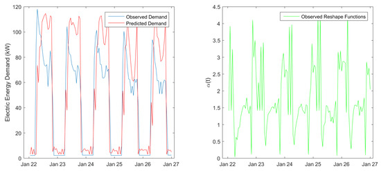
Figure 2.
Example of the observed and simulated daily energy demand (per hour) and the corresponding reshape functions for the time period 22/01/2018 to 26/01/2018.
Under this consideration, for an appropriately chosen period of time each function, should not present significant fluctuations from the reshape function that is considered as the “typical” one. Therefore, an appropriate notion of mean regarding the set of reshape functions is needed to properly define/represent the mean element in the set. The latter task requires the calculation of the mean element among a number of functions living in a space which does not necessarily has linear structure, therefore the notion of Fréchet mean needs to be exploited [29,30] for this purpose. In the context we discuss here, each reshape function is considered as a deformation to the mean element (i.e., Fréchet mean) with respect to which an appropriate notion of deviance is defined and its minimization will provide the mean element (please see [31] for technical details on this subject). A general model like the shape-invariant model [26] can be used for the parameterization of the functional characteristics of the reshape functions in order to define a consistent parametric form for the Fréchet mean. According to the shape-invariant model, shape deformations like vertical (scale) and horizontal (time) shifts can be efficiently captured. The standard shape-invariant model applied to the energy reshape functions can be written as
where denotes the mean pattern of the energy reshape function, and introduce vertical shifts parameterization, while introduces time-shift parameterization. Recall that any is considered as a deformation of the observed mean pattern (Fréchet mean) of the set . As a result, the incurred mean energy reshape function estimated by the data from the previous N days can be calculated through the equation
where vector contains all the deformation parameters. Clearly, as these parameters uniquely define the mean reshape function must be selected to minimize the mean model variance from the set , i.e., the vector is chosen as
where represents the time period within a day and represents the space of the deformation parameters which are subjected to some normalization constraints, i.e.,
Clearly, the estimation of the reshape function for the day will be used to improve the initial prediction, provided by the simulation model, for the energy demand of this day through the model
where the error term is considered as a white noise process. After the initial mean reshape function estimation from the first batch of data corresponding to the initial N days has been obtained, an exponentially weighted scheme can be used to update appropriately the reshape functions taking into account both the effect of the initial reshape function and more recent observations on the reshape function. In particular, the proposed scheme can be described through the following steps.
Initial Step
Step 1
Given the new measurement set , and .
Step 2
Set as the Fréchet mean of and with weights and , respectively.
Step 3
Given the simulation model prediction provide the improved (reshaped) prediction .
The exponential weighting is used to reduce the effect of older observations to the new predictions, i.e., for the prediction on the day using the weight parameter we could weight the most recent information (last observed reshape function ) by and the older observations by . In this manner, choosing close to 1 we allocate more weight to the most recent realizations and reduce the effect of the older observations. Otherwise, choosing close to zero, we forget the older observations with a very slow rate allowing the past information to contribute more to the prediction. Clearly, the choice of this parameter is critical to the quality of the prediction, and the final choice of this parameter depends strongly to the nature of the application that the prediction model is employed to. Note also that at each step the Fréchet mean of previous reshape functions is taken into account as an observation through the term although it is not. However, this modification allows to simultaneously condense and appropriately weight (according to our preferences provided by the choice of ) the past information into a single term.
2.2.2. The Weighted Shape Model Approach
In practice, it has been proved that there are periods of time that the prediction models do not provide reliable predictions and they may significantly deviate from the true situation. An example of such a situation is the energy demand prediction of the building during the period of summer holidays discussed in Section 3. In such cases, it is very important to quickly perceive when this happens and rapidly adjust the prediction to an acceptable level of deviance from the reality. For such purposes, we present here a small variation of the scheme presented in Section 2.2.1 where a weighted version of the reshape model is used.
The main idea is to divide the prediction into two parts: (a) the prediction provided by the reshape model and weight it by a proportion and (b) the prediction provided by previous observed energy shapes (measurements only) weighted by the proportion . For the second part, the same procedure that used for the estimation of the mean reshape function is used, i.e., given the past measurements of the daily energy shapes their Fréchet mean is estimated by (19)–(20) substituting with . The Fréchet mean in this case is interpreted as the most typical energy shape observed in the previous days without taking into account any information provided by the energy simulation model (predictive model). Then, one could shape the prediction either by constantly setting the weighting parameter w to a specific value or by changing this value each time new data become available to adjust the weighted shape model as close as it is possible to the true situation as observed until that time instant. Such a weight allocation criterion could be constructed as follows. Define by the weighted prediction, where denotes the mean energy shape as estimated until day j and denotes the shape model’s prediction for the day derived from the approach discussed in Section 2.2.1. Then, given the measurement of the day , , the weight w for the next prediction (i.e., the day ) is chosen as the minimizer to the criterion
Clearly, if the prediction provided by the simulation model is completely misplaced, then this criterion will act rapidly as a safety filter and will provide a prediction that is based more on the empirical data (previously observed energy shapes); otherwise, the prediction will be based on the simulation model. Therefore, criterion (23) will act as a detection mechanism of significant inconsistencies of the estimates provided by the simulation model and if such a significant shift occurs, will immediately properly adjust the prediction and improve its accuracy. Moreover, monitoring the value of w for a reasonable period of time, provides a measure of efficiency for the prediction model that is used. Ideally, we expect the value of w to remain in high levels (near to 1) except of some periods that major changes happen where the simulation model has not yet re-adjusted.
2.3. Postprocessing Using Kalman Filtering: The General Algorithm, Capabilities and Areas of Application, and the Filter Proposed for the Present Work
Numerical simulation models in several applications, including energy prediction systems, are exposed to systematic or non-systematic biases, an issue in which a wide number of internal or external parameters are involved: inability of simulating sub-scale phenomena, limitations in the parameterization of all the engaged parameters, and numerical schemes problems can be listed among them.
Towards the limitation of the problems above and in the framework of integrated forecasting systems, statistical postprocesses and bias removal techniques have a critical role. In particular, Kalman filters [32,33,34] provide a very popular approach for systematic bias removal, combining recursively available records with direct modeled outputs, by using weights that minimize the corresponding biases, requiring limited CPU resources and data backlog. Kalman filters have been successfully applied to a wide number of numerical models including atmospheric parameters (see, for example, [35,36,37,38,39]), sea state (see, e.g., [40,41,42]), extreme events (see, e.g., [43,44]), as well as renewable power resources (see, e.g., [45,46,47]). A general description of the basic Kalman filter algorithm is summarized below.
The main target is the simulation of two parameters that evolve in time in parallel. The state vector x and the observation corresponding y. The change of the two processes in time are described by the system and the observation equations, respectively:
The coefficient matrices, and , are defined as the system and the observation matrix, respectively. The corresponding covariance matrices , of the random vectors and , respectively, should be determined before the application of the filter while and need to be independently distributed according to Gaussian probability laws. The Kalman filter theory provides a method for the recursive estimation of the unknown state utilizing all the observation values y up to time t. The following equations describe a full integration step of the Kalman algorithm.
where
and the covariance matrix of the unknown state x is given by
where
In the present work, a linear filter has been adopted for the reduction of possible systematic biases in previous simulations steps. In particular, the estimation of the bias in time is estimated by means of the direct model output (where ):
The above provides the observation equation of the filter with observation matrix and state vector . The covariance matrices and of the state and observation errors are estimated by utilizing a training window for the observed and modeled data (see [38,41,42]). The estimated by the filter bias values are utilized for the improvement of model outputs in the next time steps. It is worth noticing that the optimum training windows as well as initial values are case sensitive and should be estimated separately for every application under study.
3. Test Cases and Results
In this section, the proposed integrated model presented in Section 2 is implemented to the prediction of the daily and hourly energy demand of Leaf Lab for the time period 2017–2018.
The Leaf Lab is an industrial Near-Zero Energy Building (NZEB) of 6000 m total floor area, integrating energy efficiency measures, advanced automations, renewable energy generation, and storage. The building envelope is highly insulated and consists of walls and double glazed windows with U values of 0.226 W/mK and 1.793–3.194 W/mK, respectively. The HVAC system of the Leaf Lab is composed of ground water source heat pumps with a nominal heating COP of 4.8 and a cooling EER of 6.2–7. The HVAC is coupled to a thermal storage water tank which is heated or cooled using excess PV power. The roof of the Leaf Lab is covered by a PV system of 236.5 kWp. Energy systems are integrated by MyLeaf platform, which allows monitoring of measurements and advanced control functions [48]. Leaf lab is part of the Leaf Community, a microgrid integrating industrial and office buildings with various renewable energy systems (biPVs, tracker PVs, and micro-hydro power system), storage (electrochemical and thermal), and electric vehicles [49]. A complete description of the Leaf Lab and systems installed along with details of the building modeling and validation procedure are available in [50]. The 3D representation of the Leaf Lab simulation model is presented in Figure 3.
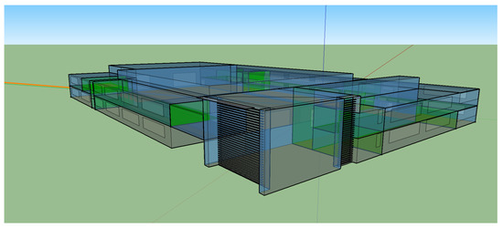
Figure 3.
The Leaf Lab 3D simulation model.
First, an indicative analysis is performed to the initial simulation model outputs comparing to the energy demand measurements to reveal and discuss the weak points of the non-optimized simulation model (SM) and what improvements are obtained from its optimized version (OSM) discussed in Section 2.1. Next, we present the improvements in energy prediction that are obtained by adopting the shape modeling approach (Section 2.2) and Kalman filtering (Section 2.3) in the postprocessing stage. For the model performance assessment, standard statistical indices are incorporated that are widely used for measuring the performance of prediction models. Let us denote by the under study model predictions for the energy demand at certain time instants and as the true (measured/observed) energy demand stature at the same time instants. In particular, the following statistical indices are used.
- Prediction Bias, , indicating any systematic underestimation or overestimation of the quantity of interest.
- Mean Absolute Error, , indicating the mean absolute deviance of the model predictions from the true value.
- Root Mean Squared Error, , indicating the mean squared deviance of the model predictions from the true value.
- Nash–Sutcliffe model efficiency coefficient, which is used to assess the predictive power of the model:taking values on where an index equal to zero corresponds to a perfect prediction whereas values below zero corresponds to the case where the prediction model was outperformed by a reference model .
3.1. Indicative Analysis of the Initial Simulation Results: Revealing the Weak Points
A snapshot of the simulated versus measured HVAC electric power for working days of the week from 7/8/17 to 11/8/17 is presented in Figure 4. Simulated versus actual measured total HVAC electric energy consumption for the year 2017 is presented in Figure 5a. It is noted that there are significant deviations on a monthly basis which become more evident for months of unstable environmental conditions such as March, May, and September, as well as in February. The total annual HVAC electrical energy consumption in 2017 for Leaf Lab was 285,719 kWh (47.61 kWh/m), whereas the respective simulated value is 197,305 kWh (32.88 kWh/m). The corresponding values excluding weekends is 232,669 kWh and 180,522 kWh, which correspond to an unacceptably high level of monthly CVRMSE equal to 40.7%.
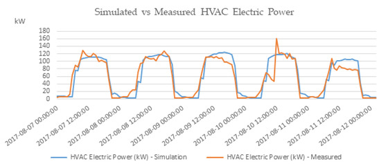
Figure 4.
Simulated vs. measured HVAC electric power for the week from 7/8/17 to 11/8/17.
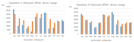
Figure 5.
Measured total HVAC electrical energy consumption for the year 2017 versus: (a) initial model (baseline) (left plot) and (b) parameterized model (optimized) (right plot).
Following parameterization of the model monthly deviation in HVAC, electric energy consumption are minimized to a percentage difference ranging from 1.78% in February to 30.28% in September and an acceptable CVRMSE of 13.89% (Figure 5b). Total simulated HVAC electric energy in this optimized case is 252,689 kWh or 221,946 kWh excluding weekends associated to a percentage difference of 11.5% and 4.6%, respectively.
Table 1 contains monthly measured HVAC electrical energy consumption values and the corresponding simulated ones obtained from the baseline and optimized models for 2017.

Table 1.
Monthly measured HVAC electrical energy consumption values and the corresponding simulated ones obtained from the baseline and optimized models for 2017.
Similarly, results from the initial simulation in 2018 are presented in Figure 6a. Notably, there are significant levels of underprediction especially in April, May, and September. The total annual HVAC electrical energy consumption in 2018 for Leaf Lab was 290,760 kWh (48.46 kWh/m), whereas the respective simulated value is 221,136 kWh (36.85 kWh/m), which equals a percentage difference of 23.9%. The corresponding values excluding weekends is 250,042 kWh and 200,461 kWh, which correspond to an unacceptably high level of monthly CVRMSE equal to 31.42%.
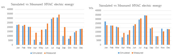
Figure 6.
Measured total HVAC electrical energy consumption for the year 2018 versus: (a) initial model (baseline) (left plot) and (b) parameterized model (optimized) (right plot).
Table 2 contains monthly measured HVAC electrical energy consumption values and the corresponding simulated ones obtained from the baseline and optimized models for 2018.
Table 2.
Monthly measured HVAC electrical energy consumption values and the corresponding simulated ones obtained from the baseline and optimized models for 2018.
An intensive search of the parameters that affect the daily, monthly, and annual power distribution profiles is presented in the following to improve the initial results of the model based by minimizing deviation from HVAC power consumption data. Through trial and error various combinations and fine-tuning of the all of key parameters are carried out to reach the optimum results both when assessing deviation at intra-day, monthly, and annual timescale. During this approach, the two key parameters identified as critical to decreasing the model’s deviation from actual metered energy consumption are the COP and infiltration rates. COP nominal values are initially used but as they are representative of standard conditions, validation is required to better estimate their performance in dynamic conditions. Furthermore, the energy model uses performance curves to simulate the dynamic behavior of heat pump systems which is hard to define in the absence of very elaborate measuring equipment especially for systems customized to provide heating and cooling for large facilities. Besides, fine-tuning model parameters to match the actual performance in such systems is further justified by the fact that user behavior is not recorded and even if it was, modeling of such a complex activity is not feasible provided the current features of energy building software tools. Indicatively, the opening of external windows, the entry (or exit) of people or industrial equipment and the manual control of the temperature set point in the various thermal zones are some factors of uncertainty as to the actual thermal energy exchanges of a building such as the Leaf Lab.
Following careful fine-tuning of the model, simulation results are improved as shown in Figure 6b. Specifically, parameters related to the infiltration, ventilation, internal loads (electric equipment and lighting), and occupancy of the various zones were varied until the best possible correlation was established. Although some noticeable at monthly level differences remain especially in April and May, overall, the simulated results approach actual measured values as revealed by CVRMSE of 14.33%. In Figure 7, simulated versus measured HVAC electric power for a week in November 2018 is presented. In this case, the simulated pattern follows the actual measured values; however, there clear deviations especially with respect to the peaks early in the morning and late in the afternoon are observed.
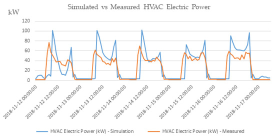
Figure 7.
Simulated versus measured HVAC electric power for the week from 12/11/18 to 17/11/18.
In Figure 8 and Figure 9, the evolution of statistical indices (Bias, MAE, and RMSE) regarding the deviance of the initial simulation model is illustrated, and its optimized parameterized version comparing to the measured energy demand for the years 2017–2018. With regards to Bias, the optimized model significantly outperforms the initial energy model of the building which underestimates energy consumption for most months in 2017. Concerning MAE and RMSE, it is demonstrated that the optimized model generally performs better except for months March, April, October, and November for which the initial model performs slightly better. Similarly, in 2018, the results of the optimized model are associated with a Bias error of lower magnitude for months from April to October. MAE and RMSE, in this case, are lower in the case of the optimized model compared to the baseline model for months from February to November. In contrast, the initial model performs marginally better for estimating energy consumption in January, October, and November.
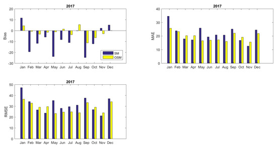
Figure 8.
Statistical error indices for the energy prediction through the simulation model (SM) and the optimized simulation model (OSM) for the year 2017 (per month).
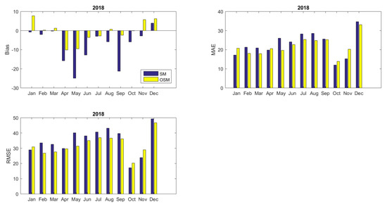
Figure 9.
Statistical error indices for the energy prediction through the simulation model (SM) and the optimized simulation model (OSM) for the year 2018 (per month).
3.2. Diagnostic Results for the Complete Model Outputs
In this section, we discuss the improvements obtained to the energy consumption prediction for the Leaf Lab building for the time period 2017–2018 by implementing the postprocess part of the integrated model, i.e., the shape modeling approach and Kalman filtering. For convenience, let us introduce the abbreviations (SM) for the initial (benchmark) simulation model, (OSM) for the optimized/parameterized simulation model, (RS) for the reshaped simulation model, (w-RS) for the weighted reshaped model, and (KF-RS) for the integrated model by implementing Kalman filtering at the later stage of the reshape model output. For illustration purposes, we divide our analysis into two parts: (a) regarding the intra-day (hourly) energy demand prediction and (b) regarding the prediction of daily summary of the energy demand (total energy demand on the whole day).
3.2.1. Evaluating Intra-Day Energy Demand Predictions
In Table 3, the yearly diagnostic results of the intra-day energy demand predictions (hourly), provided by all incorporated prediction models for the years 2017 and 2018, are presented. Note that the NSE coefficient is calculated using as reference model the initial simulation model (SM). Based on the various indices, it is clearly demonstrated that the reshape modeling provides much higher levels of accuracy compared to the model’s simulated outputs. Specifically, it is observed that RMSE in both years is reduced ~50%. The Kalman filtering procedure does not further improve the intra-day prediction performance of the reshaped model, indicating that the utilized shape model filters out efficiently most systematic sources of error affecting the intra-day (hourly) energy demand prediction.
Table 3.
Model diagnostic results for intra-day energy demand predictions (hourly) for the years 2017 and 2018.
Figure 10 and Figure 11 illustrate the monthly Bias, MAE, and RMSE values for both reshaped models RS and w-RS computed for the intra-day performance of the models compared to the results obtained by the optimized simulation model (OSM). Both reshaped models perform better as all statistical indices in the majority of cases are significantly improved indicating the superior predictability of the reshaped approach.
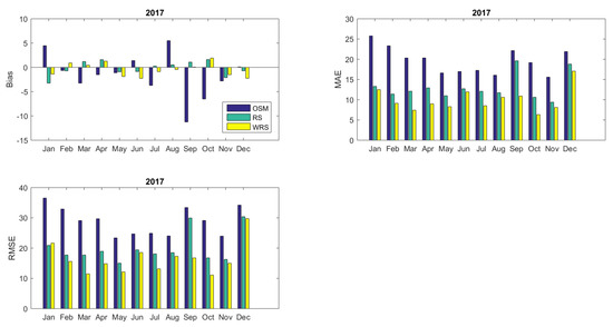
Figure 10.
Statistical error indices for the Reshaped Simulation Model (RS) and the Weighted Reshaped Simulation Model (w-RS) for the year 2017 (per month).
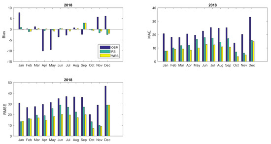
Figure 11.
Statistical error indices for the Reshaped Simulation Model (RS) and the Weighted Reshaped Simulation Model (w-RS) for the year 2018 (per month).
3.2.2. Evaluating Daily Summaries Energy Demand Predictions
At a second stage, we are interested in the performance of the incorporated models in predicting the total energy demand per day. The same model approaches are tested, and their results are illustrated in Table 4. In this case, the Kalman filtering step further improves the prediction since the model biases are reduced significantly and the best NSE values are obtained through the KF-RS model. This happens because although the RS and w-RS models efficiently capture intra-day effects in the shape of the energy demand, when we are interested in the daily summary, these effects are mutually canceled and become obsolete. However, the KF-RS model, in general, improves the average biases, as it detects these inefficiencies as systematic ones from the perspective of daily summaries, and therefore it further improves the model outputs.
Table 4.
Model diagnostic results for the predictions on the daily energy demand (summaries) for the years 2017 and 2018.
In Figure 12 and Figure 13, the performance of the KF-RS model in predicting the daily energy demand (summaries) is illustrated, comparing again to the OSM model. It is evident that the later model is significantly improved by correcting major inconsistencies in certain time periods throughout the year and more accurately approximating the true levels of energy needed. In particular, for special cases where systematic biases are present (see, e.g., highlighted periods in Figure 12 and Figure 13), the KF-RS model proves able to eliminate systematic over- or underestimations.
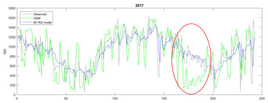
Figure 12.
Prediction of the daily energy demand (summary) obtained by optimized simulation model (OSM) and Kalman filter-enhanced reshaped simulation model (KF-RS) for the year 2017.
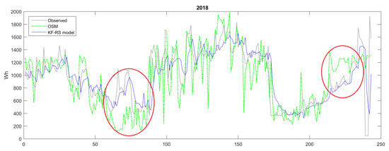
Figure 13.
Prediction of the daily energy demand (summary) obtained by optimized simulation model (OSM) and Kalman filter-enhanced reshaped simulation model (KF-RS) for the year 2018.
4. Conclusions
In this paper, validation of the building energy model of an industrial near-zero energy building is investigated over a two-year period. It is demonstrated that manual extensive fine-tuning of key model parameters is valuable to improve initial overall error levels using trial and error of key parameters. However, this process requires a high level of expertise, deep knowledge of the facility under study, and it is very time-consuming. Furthermore, it is demonstrated that systematic deficiencies continue to occur even after careful fine-tuning of key model parameters. On the one hand, this is due to the complicated issue of modeling the behavior of users as well as of equipment use in a large industrial facility. On the other hand, the dynamic performance of custom-built HVAC systems requires specific measurements if it is not to be solely defined at a high level and modeled based on nominal performance coefficients. To address this problem two modeling approaches are integrated: (a) the shape and weighted shape model and (b) Kalman filtering postprocessing. The above methods are applied in a postprocessing stage, which is tested and evaluated. Initial, optimized simulation results and results from postprocessing are analyzed compared with the aid of bias error, mean absolute error, root mean squared error, and the Nash–Sutcliffe model efficiency coefficient. Results are explored to demonstrate the effectiveness of the method in capturing and reducing intra-day systematic deviations as well as the overall performance gap. Overall, the proposed integrated approach proves to be very effective in eliminating systematic over or under estimations and critically reduces the magnitude of deviations and as a result significantly reduces the performance gap compared to the optimized simulation model. In particular, the integrated prediction model succeeded in reducing the RMSE (in mean values) approximately 39% and 43% for the hourly predictions in years 2017 and 2018, respectively, and approximately 32% and 25% for the daily energy demand for the same years which are rather impressive improvements. Note also that in all cases, the integrated prediction model substantially increased model efficiency coefficient (NS) at least 70% comparing to the efficiency of the optimized simulation model (OSM). The proposed approach is applicable in several types of buildings (i.e., residential, commercial, public, etc.) provided that reliable data of energy consumption and of human activity are available over a significant period of time (ideally more than one year). As a future step, the presented approach could be deployed and tested across several types of buildings that fall into different energy efficiency categories to assess its performance over a wide spectrum of applications.
Author Contributions
Conceptualization, N.K., G.I.P., D.K., G.N.G. and A.N.Y.; Data curation, N.K., G.I.P. and D.I.; Formal analysis, N.K., G.I.P., G.N.G. and A.N.Y.; Funding acquisition, N.K., D.K. and C.C.; Investigation, N.K., G.I.P., D.K., G.N.G. and A.N.Y.; Methodology, N.K., G.I.P., D.K., G.N.G. and A.N.Y.; Project administration, C.C.; Resources, D.K., G.N.G., D.I., C.C. and A.N.Y.; Supervision, D.K. and C.C.; Validation, G.I.P.; Visualization, N.K. and G.I.P.; Writing – original draft, N.K., G.I.P., G.N.G. and A.N.Y.; Writing – review & editing, N.K., G.I.P., D.K., G.N.G., D.I. and A.N.Y. All authors have read and agreed to the published version of the manuscript.
Funding
This project has received funding from the European Union’s Horizon 2020 research and innovation programme under the Marie Skeodowska-Curie grant agreement No 645677.
Conflicts of Interest
The authors declare no conflict of interest.
References
- International Energy Agency. Available online: https://www.iea.org/topics/energy-efficiency/buildings/ (accessed on 18 September 2019).
- Athienitis, A.K.; O’Brien, W. Modeling, Design, and Optimization of Net-Zero Energy Buildings; Wiley Online Library: Hoboken, NJ, USA, 2015. [Google Scholar]
- Zhao, H.x.; Magoulès, F. A review on the prediction of building energy consumption. Renew. Sustain. Energy Rev. 2012, 16, 3586–3592. [Google Scholar] [CrossRef]
- Santamouris, M. Advances in Building Energy Research; Taylor & Francis: Hoboken, NJ, USA, 2010; Volume 4. [Google Scholar]
- Foucquier, A.; Robert, S.; Suard, F.; Stéphan, L.; Jay, A. State of the art in building modeling and energy performances prediction: A review. Renew. Sustain. Energy Rev. 2013, 23, 272–288. [Google Scholar] [CrossRef]
- SPARK 2.0 REFERENCE MANUAL Simulation Problem Analysis and Research Kernel. Available online: https://simulationresearch.lbl.gov/VS201/doc/SPARKreferenceManual.pdf (accessed on 11 November 2019).
- Harish, V.; Kumar, A. A review on modeling and simulation of building energy systems. Renew. Sustain. Energy Rev. 2016, 56, 1272–1292. [Google Scholar] [CrossRef]
- Naji, S.; Keivani, A.; Shamshirband, S.; Alengaram, U.J.; Jumaat, M.Z.; Mansor, Z.; Lee, M. Estimating building energy consumption using extreme learning machine method. Energy 2016, 97, 506–516. [Google Scholar] [CrossRef]
- Robinson, C.; Dilkina, B.; Hubbs, J.; Zhang, W.; Guhathakurta, S.; Brown, M.A.; Pendyala, R.M. Machine learning approaches for estimating commercial building energy consumption. Appl. Energy 2017, 208, 889–904. [Google Scholar] [CrossRef]
- Amasyali, K.; El-Gohary, N.M. A review of data-driven building energy consumption prediction studies. Renew. Sustain. Energy Rev. 2018, 81, 1192–1205. [Google Scholar] [CrossRef]
- Wei, Y.; Zhang, X.; Shi, Y.; Xia, L.; Pan, S.; Wu, J.; Han, M.; Zhao, X. A review of data-driven approaches for prediction and classification of building energy consumption. Renew. Sustain. Energy Rev. 2018, 82, 1027–1047. [Google Scholar] [CrossRef]
- De Wit, S.; Augenbroe, G. Analysis of uncertainty in building design evaluations and its implications. Energy Build. 2002, 34, 951–958. [Google Scholar] [CrossRef]
- Ryan, E.M.; Sanquist, T.F. Validation of building energy modeling tools under idealized and realistic conditions. Energy Build. 2012, 47, 375–382. [Google Scholar] [CrossRef]
- Maile, T.; Bazjanac, V.; Fischer, M. A method to compare simulated and measured data to assess building energy performance. Build. Environ. 2012, 56, 241–251. [Google Scholar] [CrossRef]
- Coakley, D.; Raftery, P.; Keane, M. A review of methods to match building energy simulation models to measured data. Renew. Sustain. Energy Rev. 2014, 37, 123–141. [Google Scholar] [CrossRef]
- M & V Guidelines: Measurement and Verification for Performance-Based Contracts Version 4.0. Available online: https://www.energy.gov/sites/prod/files/2016/01/f28/mv_guide_4_0.pdf (accessed on 12 August 2019).
- Royapoor, M.; Roskilly, T. Building model calibration using energy and environmental data. Energy Build. 2015, 94, 109–120. [Google Scholar] [CrossRef]
- O’Neill, Z.D.; Bailey, T.G.; Eisenhower, B.A.; Fonoberov, V.A. Calibration of a building energy model considering parametric uncertainty. ASHRAE Trans. 2012, 118, 189–196. [Google Scholar]
- O’Neill, Z.D.; Eisenhower, B.A.; Bailey, T.G.; Narayanan, S.; Fonoberov, V.A. Modeling and calibration of energy models for a DoD building. ASHRAE Trans. 2011, 117, 358–365. [Google Scholar]
- EnergyPlusTM, Engineering Reference Documentation Version 9.1.0, National Renewable Energy Laboratory. 2019. Available online: https://energyplus.net (accessed on 12 August 2019).
- Brackney, L.; Parker, A.; Macumber, D.; Benne, K. Building Energy Modeling with OpenStudio; Springer: Berlin, Germany, 2018. [Google Scholar]
- Wand, M.P.; Jones, M.C. Kernel Smoothing; Chapman and Hall/CRC: Boca Raton, FL, USA, 1994. [Google Scholar]
- Ramsay, J.O.; Silverman, B.W. Applied Functional Data Analysis: Methods and Case Studies; Springer: New York, NY, USA, 2007. [Google Scholar]
- Gu, C. Smoothing Spline ANOVA Models; Springer Science & Business Media: Berlin, Germany, 2013; Volume 297. [Google Scholar]
- Lawton, W.; Sylvestre, E.; Maggio, M. Self modeling nonlinear regression. Technometrics 1972, 14, 513–532. [Google Scholar] [CrossRef]
- Kneip, A.; Engel, J. Model estimation in nonlinear regression under shape invariance. Annals Stat. 1995, 23, 551–570. [Google Scholar] [CrossRef]
- Gervini, D.; Gasser, T. Self-modeling warping functions. J. R. Stat. Soc. Ser. B (Statistical Methodol.) 2004, 66, 959–971. [Google Scholar] [CrossRef]
- Papayiannis, G.I.; Giakoumakis, E.A.; Manios, E.D.; Moulopoulos, S.D.; Stamatelopoulos, K.S.; Toumanidis, S.T.; Zakopoulos, N.A.; Yannacopoulos, A.N. A functional supervised learning approach to the study of blood pressure data. Stat. Med. 2018, 37, 1359–1375. [Google Scholar] [CrossRef]
- Fréchet, M. Les éléments aléatoires de nature quelconque dans un espace distancié. Ann. De L’institut Henri Poincaré 1948, 10, 215–310. [Google Scholar]
- Izem, R.; Marron, J.S. Analysis of nonlinear modes of variation for functional data. Electron. J. Stat. 2007, 1, 641–676. [Google Scholar] [CrossRef]
- Bigot, J.; Charlier, B. On the consistency of Fréchet means in deformable models for curve and image analysis. Electron. J. Stat. 2011, 5, 1054–1089. [Google Scholar] [CrossRef]
- Kalman, R.E. A new approach to linear filtering and prediction problems. J. Basic Eng. 1960, 82, 34–45. [Google Scholar] [CrossRef]
- Kalman, R.E.; Bucy, R.S. New results in linear filtering and prediction theory. J. Basic Eng. 1961, 83, 95–108. [Google Scholar] [CrossRef]
- Kalnay, E. Atmospheric Modeling, Data Assimilation and Predictability; Cambridge University Press: Cambridge, UK, 2003. [Google Scholar]
- Crochet, P. Adaptive Kalman filtering of 2-metre temperature and 10-metre wind-speed forecasts in Iceland. Meteorol. Appl. 2004, 11, 173–187. [Google Scholar] [CrossRef]
- Galanis, G.; Anadranistakis, M. A one-dimensional Kalman filter for the correction of near surface temperature forecasts. Meteorol. Appl. 2002, 9, 437–441. [Google Scholar] [CrossRef]
- Emmanouil, G.; Galanis, G.; Kallos, G. Statistical methods for the prediction of night-time cooling and minimum temperature. Meteorol. Appl. 2006, 13, 169–178. [Google Scholar] [CrossRef][Green Version]
- Galanis, G.; Louka, P.; Katsafados, P.; Pytharoulis, I.; Kallos, G. Applications of Kalman filters based on non-linear functions to numerical weather predictions. Ann. Geophys. 2006, 24, 2451–2460. [Google Scholar] [CrossRef]
- Hua, S.; Wang, S.; Jin, S.; Feng, S.; Wang, B. Wind speed optimisation method of numerical prediction for wind farm based on Kalman filter method. J. Eng. 2017, 2017, 1146–1149. [Google Scholar] [CrossRef]
- Emmanouil, G.; Galanis, G.; Kallos, G. Combination of statistical Kalman filters and data assimilation for improving ocean waves analysis and forecasting. Ocean Model. 2012, 59, 11–23. [Google Scholar] [CrossRef]
- Galanis, G.; Emmanouil, G.; Chu, P.C.; Kallos, G. A new methodology for the extension of the impact of data assimilation on ocean wave prediction. Ocean Dyn. 2009, 59, 523–535. [Google Scholar] [CrossRef]
- Galanis, G.; Chu, P.C.; Kallos, G. Statistical post processes for the improvement of the results of numerical wave prediction models. A combination of Kolmogorov-Zurbenko and Kalman filters. J. Oper. Oceanogr. 2011, 4, 23–31. [Google Scholar] [CrossRef][Green Version]
- Patlakas, P.; Drakaki, E.; Galanis, G.; Spyrou, C.; Kallos, G. Wind gust estimation by combining a numerical weather prediction model and statistical postprocessing. Energy Procedia 2017, 125, 190–198. [Google Scholar] [CrossRef]
- Samalot, A.; Astitha, M.; Yang, J.; Galanis, G. Combined kalman filter and universal kriging to improve storm wind speed predictions for the northeastern United States. Weather Forecast. 2019, 34, 587–601. [Google Scholar] [CrossRef]
- Louka, P.; Galanis, G.; Siebert, N.; Kariniotakis, G.; Katsafados, P.; Pytharoulis, I.; Kallos, G. Improvements in wind speed forecasts for wind power prediction purposes using Kalman filtering. J. Wind Eng. Ind. Aerodyn. 2008, 96, 2348–2362. [Google Scholar] [CrossRef]
- Pelland, S.; Galanis, G.; Kallos, G. Solar and photovoltaic forecasting through postprocessing of the Global Environmental Multiscale numerical weather prediction model. Prog. Photovoltaics: Res. Appl. 2013, 21, 284–296. [Google Scholar] [CrossRef]
- Stathopoulos, C.; Kaperoni, A.; Galanis, G.; Kallos, G. Wind power prediction based on numerical and statistical models. J. Wind Eng. Ind. Aerodyn. 2013, 112, 25–38. [Google Scholar] [CrossRef]
- MyLeaf Platform - Loccioni Group. Available online: https://https://myleaf2.loccioni.com (accessed on 26 July 2018).
- Provata, E.; Kolokotsa, D.; Papantoniou, S.; Pietrini, M.; Giovannelli, A.; Romiti, G. Development of optimization algorithms for the Leaf Community microgrid. Renew. Energy 2015, 74, 782–795. [Google Scholar] [CrossRef]
- Kampelis, N.; Gobakis, K.; Vagias, V.; Kolokotsa, D.; Standardi, L.; Isidori, D.; Cristalli, C.; Montagnino, F.; Paredes, F.; Muratore, P.; et al. Evaluation of the performance gap in industrial, residential & tertiary near-Zero energy buildings. Energy Build. 2017, 148, 58–73. [Google Scholar]
© 2020 by the authors. Licensee MDPI, Basel, Switzerland. This article is an open access article distributed under the terms and conditions of the Creative Commons Attribution (CC BY) license (http://creativecommons.org/licenses/by/4.0/).