Predicting Frequency, Time-To-Repair and Costs of Wind Turbine Failures

Abstract

Operation and maintenance (O&M) costs, and associated uncertainty, for wind turbines (WTs) is a significant burden for wind farm operators. Many wind turbine failures are unpredictable while causing loss of energy production, and may also cause loss of asset. This study utilized 753 O&M event data from 21 wind turbines operating in Germany, to improve the prediction of failure frequency and associated costs. We applied Bayesian updating to predict wind turbine failure frequency and time-to-repair (TTR), in conjunction to machine learning techniques for assessing costs associated with failures. We found that time-to-failure (TTF), time-to-repair and the cost of failures depend on operational and environmental conditions. High elevation (>100 m) of the wind turbine installation was found to increase both the probability of failures and probability of delayed repairs. Furthermore, it was determined that direct-drive turbines are more favorable at locations with high capacity factor (more than 40%) whereas geared-drive turbines show lower failure costs than direct-drive ones at temperate-coastal locations with medium capacity factors (between 20% and 40%). Based on these findings, we developed a decision support tool that can guide a site-specific selection of wind turbine types, while providing a thorough estimation of O&M budgets.

1. Introduction

Operation and maintenance (O&M) of wind turbines (WTs) can be a burden to wind farm operators. Many failures of wind turbines are unpredictable, and the uncertainty presents risks of loss of energy production, loss of asset and lacking O&M monetary budget. Mone et al. (2017) [1] determined O&M cost of wind turbines as high as $14.6/MWh for a 2 MW onshore wind turbine in a 200 MW-project, and $49.6/MWh for a 4.14 MW offshore wind turbine in a 600 MW-project. The corresponding total, during a 20 years-lifetime, O&M costs were around 2$M and 14.8$M for the onshore and the offshore wind turbine, respectively [1]. This was in addition to the cost for lost energy production during the failure and maintenance periods. Proactive maintenance is expected to decrease downtime and the cost of failure but the extent and frequency of needed maintenance is debatable [2,3].

There are several studies in the literature on wind turbine reliability prediction and maintenance optimization. Faultsich et al. (2011) [4] studied topographical and environmental factors causing wind turbine failures and concluded that turbines close to seawater and at high land locations (the elevation is not specified) with high wind speed suffer the highest failure rates. Wilson and McMillan (2014) [5] assessed wind farm reliability but they only used weather dependent failure rates. Slimacek and Lindqvist (2016) [6] applied Poisson and survival analyses to analyze wind turbine failure frequencies accounting for type and size of turbines, harshness of environment, time from installation, and seasonal effects. They found that lightning, icing and high wind increased the failure rate by 1.7 times. Consequently, Reder et al. (2018) [7] proposed a framework consisting of data mining and k-means clustering techniques, to determine the effects of weather conditions on wind turbine failures by analyzing Supervisory Control and Data Acquisition (SCADA) data. Contrary to Slimacek and Lindqvist, they found that wind speed did not impact failure occurrences; they also reported that failure frequencies were increased in the winter. Reder and Melero (2018) [8] proposed using Bayes Belief Networks (BBN) to predict wind turbine failures based on weather conditions. They have utilized failure data from 948 wind turbines operating during 87 wind turbine-years, and concluded that BBN is capable of reliably predicting wind turbine failures. However, their study was limited to 1.1 month of operation per turbine on average and lacked maintenance cost prediction.

Regarding the cost and benefit of preventive maintenance, Besnard (2009) [2] estimated that employing a condition monitoring system would result to savings of 190,000 € for a 3 MW wind turbine. They also determined the optimal interval for visual inspection to be four months and for blades to be one year. Ortegon et al. (2014) [3] investigated typical failure rates and maintenance cost to evaluate the cost-benefit of applying preventive maintenance. They determined that corrective maintenance would cost $511,596 if there is no preventive maintenance, whereas the total O&M cost would be $77,542 if there are two preventive maintenance events per year per turbine in its entire life using average failure probability values from various O&M databases. Leigh and Dunnett (2016) [9] developed a mathematical model for the maintenance of wind turbines considering three types of maintenance, namely periodic, conditional and corrective for an offshore 5 MW turbine. The model evaluated the number of corrective maintenances required for a lifetime of the turbine for every subsystem [9]. Carlos et al. (2013) [10] applied Monte Carlo simulations for maintenance optimization purposes using generic failure database and wind speed data from a Spanish database. They concluded that the optimum scheduled maintenance interval should be 113 days instead of a typical industry schedule of 180 days, whereas Kerres et al. (2014) [11] found that corrective maintenance done upon a failure, is a better option for a V44-600 kW turbine. Raza and Ulansky (2019) [12] applied imperfect continuous condition monitoring which considers correct and incorrect decisions about preventive maintenance for wind turbines. They concluded that a preventive maintenance could reduce the average lifetime maintenance cost 11.8 times comparing the corrective maintenance for wind turbine blades.

Overall, several of the previous studies diverse in their findings and new approaches to data analysis and modeling may be needed to provide more cohesive guidance to wind turbine O&M managers. In an effort to better elucidate O&M risks and burdens, we recently investigated the impact of climatic region and turbine gear type by using Failure Modes Effects and Criticality Analysis (FMECA) and found that colder climates have more effect on some subsystems and parts (e.g., blade shells) while turbine gear type mainly impact the frequency and repair time of subsystems and parts [13]. Subsequently, we assessed risk factors for wind turbine reliability applying survival analysis [14]. Our previous findings show that scheduled maintenance can increase the survival of a wind turbine system and electrical subsystems up to 2.8 and 3.8 times, respectively. The current study uses the risk factors determined in [13,14] to improve the prediction of the frequency of wind turbine failures and associated repair times Bayesian updating. In addition, we employ machine learning techniques on the risk factors, to assess wind turbine failure costs [13,14].

Bayesian updating has not been used before in probabilistic assessments of time-to-failure (TTF) and time-to-repair (TTR) and machine learning techniques were not used previously in determining costs of failures for wind turbines although they were used for component condition monitoring [15,16,17] and for other applications [18,19,20,21]. The major contributions of this paper are two-fold: (1) Bayesian updating is used at the first time in probabilistic assessments of time-to-failure and time-to-repair of wind turbines. (2) It is a novel use of machine learning applications to estimate cost of wind turbine failures using operational and environmental conditions.

Predicting time-to-failure, time-to-repair and cost of failures should offer valuable guidance to the wind turbine industry. Thus, the goal of this study is two-fold. Firstly, to evaluate time-to-failure (TTF) probabilities for every month of operation and estimating time-to-repair (TTR) probabilities for TTR ≤ 8 h, 8 h < TTR ≤ 16 h, 16 h < TTR ≤ 24 h, and more than 1-day time intervals based on operational and environmental conditions using Bayesian updating. Secondly, to develop a decision support tool for estimating cost of failures of wind turbines from operational and environmental conditions in a German database, using machine learning techniques. The decision support tool can be utilized by wind farm investors for site and turbine type selection and for wind farm operators for allocating O&M budgets and evaluating the cost and benefit of O&M services offered by third parties.

This paper contains six sections covering the following:

• The first section introduces wind turbine O&M costs and related literature review of reliability prediction and modeling; maintenance optimization and cost and benefit of preventive maintenance. The goal of the paper is also stated in the first section.
• In the second section, materials, data and variable categories are explained.
• In the third section, methodologies for failure frequency, time-to-repair prediction and cost of failure estimation methods are explained.
• In the fourth section development of a decision tool is explained step-by-step.
• The fifth section presents the results based on two different applications of Bayesian updating and machine learning techniques.
• In the last section conclusions are drawn.

2. Data and Selected Variables

2.1. Reliability Data

The Wind Monitor and Evaluation Program (WMEP) database, which is utilized as reliability data in this study, is a comprehensive maintenance database covering 19 years (1989 to 2008) of wind turbine operations in Germany [4]; unfortunately, this database has not been extended to recent years. Twenty-one wind turbines with capacities of 500 kW, 600 kW and 1500 kW are selected as representative of two different designs, namely geared and direct-drive turbines. Thirteen turbines have 500 kW, 2 turbines have 600 kW and 6 turbines have 1500 kW capacities. In this study the turbines are surveyed for all their maintenance activities, and this created 753 O&M data points.

The aim of this study is to identify and evaluate methodologies for predicting wind turbine failure frequency, time-to-repair and cost of repair. The only detailed data available to us for illustrating the considered methodologies covered the period 1989–2008. Considering the evolution of wind turbines in recent years, the results from these data may not be applicable to current wind turbines. However, data descriptive of newer types can be used in the methodologies we presented to derive more up to date results.

2.1.1. Selected Variables

Six independent variables are selected for determining factors affecting wind turbine reliability. These variables are in two main categories which consist of operational and environmental conditions. Operational factors include turbine design type, number of previous failures (NOPF) and capacity factors (CF), whereas environmental factors include geography, mean annual wind speed (MAWS) and climatic regions of turbine locations.

2.1.2. Operational Variables

Turbine design type: There are two operational designs represented in the WMEP database; these are of geared-drive and electrically induced direct-drive turbines.

Number of previous failures (NOPF): Operation cases are distinguished in low (0–20) and high-number of previous failures (21–more) there is a clear distinction between time-to-failure values of two cases of turbines with less than or equal to 20 and more than 20 failures.

Capacity factor (CF): Wind turbine operation cases are divided into three categories; low (20% > CF), medium (20 ≤ CF ≤ 40%) and high (40% ≤ CF) capacity factors.

2.1.3. Environmental Variables

Geography: Geographical regions are categorized as coastal, high inland and low inland [4]. Coastal turbine operations take place within 20 km of coastal region and less than or equal to 100 m elevation from sea level, high inland turbine operations take place at locations with elevation of more than 100 m from sea level, with the rest of turbine operations classified as low inland turbine operations.

Mean Annual Wind Speed (MAWS): Turbine operations are classified into low level (<6.25 m/s) and high level (≥6.25 m/s) based on the values from global wind atlas [22]; these wind speed levels correspond to the hub height of the wind turbines.

Climatic region: Koppen-Geiger climatic regions are utilized for climate classification [13]. Germany includes temperate and cold Koppen-Geiger climatic regions. For the cold climatic region, average temperature of the coldest month is less than or equal to 0 °C whereas for the temperate climatic region, average temperature of the coldest month is between 0 °C and 18 °C [23].

In this study we have employed environmental variables with long term effects aiming to develop models for predicting monthly or annual wind turbine operation. However, additional higher-resolution environmental data could be used in the outlined methodology in order to derive short term failure prediction models.

The number of data and their share in the considered categories of variables are shown in

Table 1. Summary of number of data points based on variables.

Variable	Categories	Frequency	Share
Design type	Direct	602	80%
	Geared	151	20%
Geography	Coastal	325	43%
	High Inland	311	41%
	Low Inland	117	16%
Number of previous failures	(0–20)	232	31%
	(21–more)	521	69%
Mean annual wind speed	High	332	44%
	Low	421	56%
Climatic regions	Cold	299	40%
	Temperate	454	60%
Capacity factor	High	112	15%
	Low	328	43%
	Medium	313	42%

.

3. Methodology

Two approaches were applied to determine wind turbine frequencies of failure and associated times to repair; namely Bayesian updating and machine learning. A Bayesian updating is used to predict discrete time-to-failure and time-to-repair probabilities for wind turbines based on their known operational and environmental parameters. Cost of failures are predicted from the probabilities of time-time-to-failure and of time-to-repair which are derived by machine learning methods. These methods included logistic regression, artificial neural network, k-nearest neighbor and support vector machine learning.

3.1. Turbine-Based Failure Frequency and Time-to-Repair Prediction

3.1.1. Bayes Theorem

The Bayes theorem is first introduced by Thomas Bayes in 1950s and has been used in various applications. In statistics, the Bayesian approach is used to utilize prior knowledge and data from current experiment (x) to obtain posterior distribution of unknown parameter θ [18]. An important advantage of Bayesian inference is that it enables to update the probability of a failure when more data are available [19]. Let P(θ) represents the prior distribution of θ and let L(x, θ) denote the likelihood function and P(θ|x) is posterior distribution then Bayes theorem can be expressed as in the Equation (1) [18]:

$$\mathrm{P}(\mathsf{\theta }|x)=\frac{L(x,\mathsf{\theta })\mathrm{P}(\mathsf{\theta })}{{\displaystyle {\int }_{-\infty }^{\infty }L(x,\mathsf{\theta })\mathrm{P}(\mathsf{\theta })\mathrm{d}\mathsf{\theta }}}$$

(1)

3.1.2. Likelihood Function

For observed data, x, the function L(x, θ) = f(x|θ) which is considered as a function of θ is called as likelihood function. Given a set of observed data x₁, x₂, x₃, …, x_n which represent a random sample from a population of X with principal density f_x(X), the probability of observing this set of variables assuming that the parameter of the distribution is θ, is given in Equation (2) [18].

$$\mathrm{L}(x,\mathsf{\theta })={\displaystyle {\prod }_{i=1}^n{f}_x}(x_i|\mathsf{\theta })$$

(2)

3.1.3. Prior Knowledge

In Bayesian approach, prior knowledge comes from historical data, prior beliefs or previous work. A prior distribution, P(θ), which is so-called conjugate prior simplifies the application of Bayes theorem for obtaining posterior distribution. For instance, the class of normal densities is a conjugate family for normal priors which can be used for obtaining posterior density of θ given x is normal [21].

3.1.4. Posterior Distribution

Posterior distribution, P(θ|x), is calculated by Equation (1) and represents combination of beliefs from the prior knowledge about θ and beliefs which come from observed sample data x [19].

3.1.5. Beta Distribution

In probability theory and statistics beta distribution is used for binomial distributions which include discrete data. Since we consider discrete number of turbine-failures for time-to-failure and time-to-repair we use beta distribution for prior and posterior distributions in this study. Beta distribution has two parameters, namely α and β which control the shape of the distribution [24]. A Keisan-Casio online calculator is utilized for posterior beta distribution calculations [25].

3.1.6. Bayesian Updating

Generic scheduled maintenance interval for wind turbines in the industry is every three months for the first year of operation and after that every six months or every year depending on the turbine type [3]. To capture these schedules, we examined the failure probabilities on a monthly basis. Estimated probabilities of failure for the first seven months of operation at high inland locations of direct-drive wind turbines, are shown in

Table 2. An example of calculations for monthly probability of failure.

TTF (months)	Number of WT-Failures	Summation of WT-Failures (z)	Total Number of WT-Failures–Summation of WT-Failures (N–z)	Alpha (α)	Beta (β)	Probability of Failure
1	173	173	65	174	66	0.73
2	35	208	30	209	31	0.87
3	17	225	13	226	14	0.95
4	7	232	6	233	7	0.97
5	3	235	3	236	4	0.99
6	1	236	2	237	3	0.99
7	2	238	0	239	1	1

. There were 238 wind turbine-failures in total, of which 173 occurred over the course of the first month of operation. A uniform distribution was assumed for prior knowledge, since there were not prior monthly-based failure data. Therefore, alpha and beta values are added to 174 and 66, respectively which gives a 73% probability by using beta distribution mode value (Beta (174, 66)) [15]. This calculation is repeated for the rest of the months in a similar way. TTR probabilities are estimated by the same approach, considering time-to-repair intervals of TTR ≤ 8 h, 8 h < TTR ≤ 16 h, 16 h < TTR ≤ 24 h, and longer than 1-day. The rationale behind these intervals is that maintenance work shifts are mostly allotted for eight hours in the wind industry.

3.2. Predicting Cost of Failures

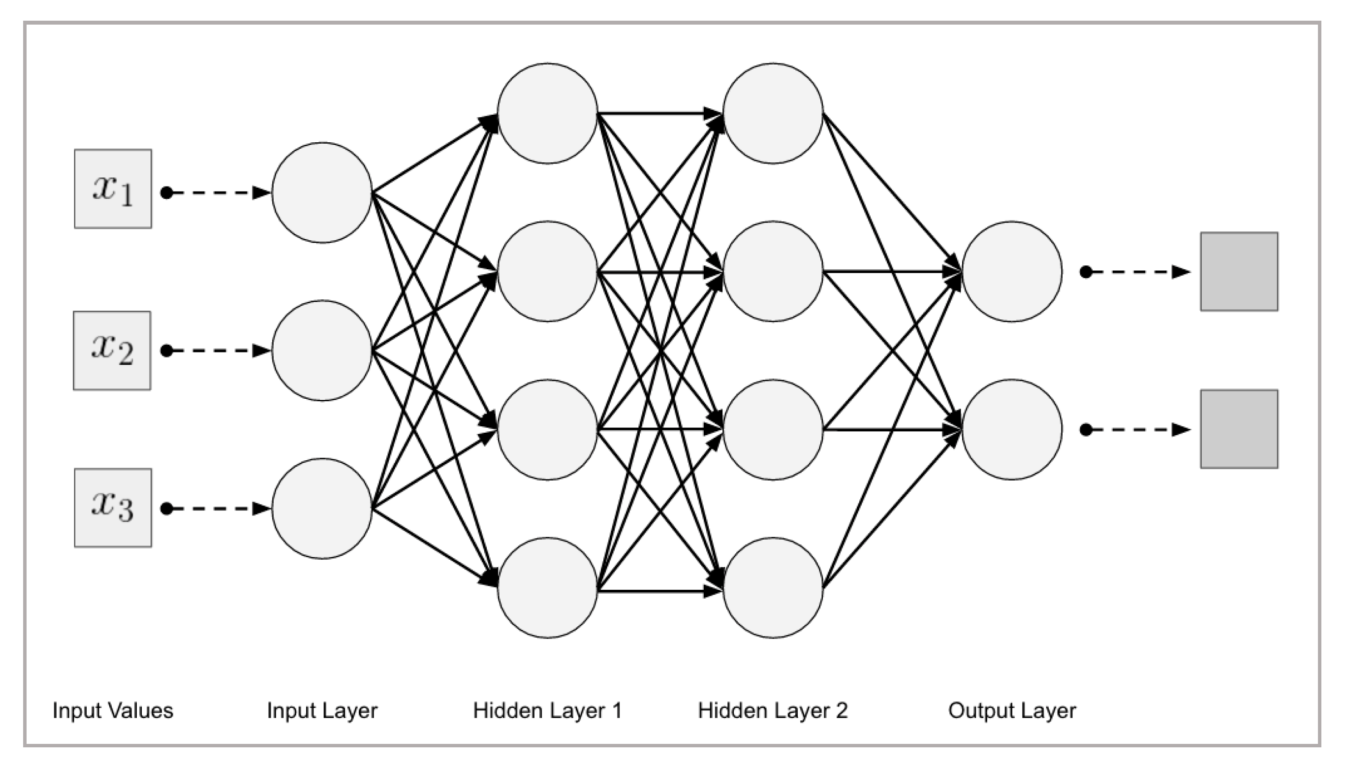
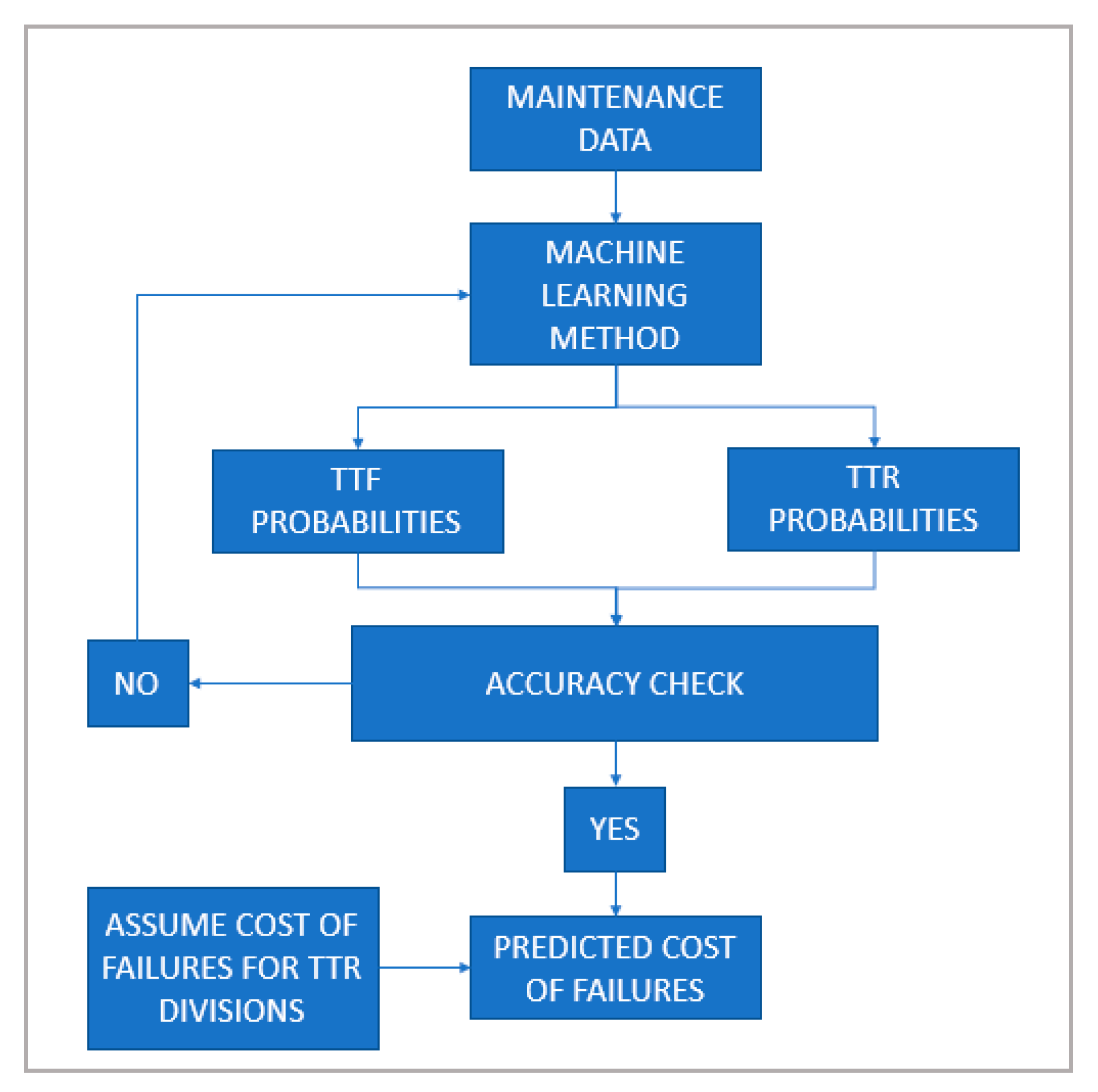
To predict the cost of failures, time-to-failure and time-to-repair, probabilities are evaluated for every combination of operational and environmental conditions by using machine learning methods; subsequently, the results are multiplied by the cost of failure for each capacity factor. Time-to-failure probabilities are estimated based on the classes of less than 60-days of operation and more than 60-days of operation since the mean value of time-to-failure of all operations is 60 days. Time-to-repair probability classes are TTR ≤ 8 h, 8 h < TTR ≤ 16 h, 16 h < TTR ≤ 24 h, and more than 1-day. Figure 1 shows a schematic illustration of a machine learning method while Figure 2 shows the schematic of developing the decision support tool.

3.2.1. Machine Learning Methods

Four machine learning methods namely logistic regression (LR), artificial neural network (ANN), k-nearest neighbor (kNN) and support vector machines (SVM) are used in this study. Machine learning methods are applied to determine the output probabilities based on input variables. The input parameters are operational and environmental variables which are given in Table 1. Output values are probability of having a failure within 60 days of operation and time-to-repair probabilities based on the time intervals which are TTR ≤ 8 h, 8 h < TTR ≤ 16 h, 16 h < TTR ≤ 24 h.

3.2.2. Logistic Regression (LR)

Logistic regression is a machine learning method which examines relationship between some input parameters and outcomes [26]. In this study, input parameters are operational and environmental variables while outcomes are failing or non-failing within 60 days of operation and time-to-repair intervals. The procedure for best fitting is done by applying several iterations until the outcome prediction ability is maximized. The mathematical expression of logistic regression is give in Equation (3).

$$\mathrm{Log}(\frac{p}{1-p})=B_0+B_1{X}_1+\dots +B_n{X}_n$$

(3)

where B₀ is a constant B₁, B₂, …, B_n are regression coefficients of the variables X₁, X₂, …, X_n. Therefore, probability of X can be calculated as in Equation (4):

$$\mathrm{P}(X)=\frac{e^{B_0+B_1{X}_1+\cdots +B_n{X}_n}}{1+e^{B_0+B_1{X}_1+\cdots +B_n{X}_n}}$$

(4)

Logistic regression (LR) uses maximum likelihood method to produce a best-fitting function to the data [18]. The procedure for best fitting is applied by several iterations to maximize the probability of the observed data to be part of the correct classified outcome given the regression coefficients.

3.2.3. Artificial Neural Networks (ANN)

The Artificial Neural Network (ANN) is a machine learning technique to model complex problems and predict outcomes utilizing collected data and independent variables [26]. The method mimics the learning and recalling behavior of human brain which consists of massive number of neurons [24]. Neurons in ANN are fully connected within three different layers, namely input layer, hidden layers and output layer as illustrated in Figure 1 [26].

Input layer has all information from the input pattern whereas hidden layer connects the input layer to the output layer by an activation function and the outcome layer transforms the hidden layer activation into the scale of desired output. The most widely used neural network which is multi-layer feed forward (MLF) with back propagation learning is used in this study. The activation function is selected as hyperbolic tangent because of its differentiable nature and use of classification purpose. The neural networks algorithm repeats feed-forwarding and back propagating until it minimizes the outcome error [26].

3.2.4. K-nearest Neighbor (KNN)

K-nearest neighbor (KNN) is a simple and widely used machine learning technique. The algorithm classifies an unknown object based on the highest vote of classes from k number of neighbors [27]. The training process aims to maximize the prediction accuracy for all data points training with different number of k’s. The steps in the KNN algorithm are as follows [28]:

• 1st step: Calculating the distances from all data point to the data point of interest.
• 2nd step: Ranking all the distances.
• 3rd step: Determining the optimal k value by training the data set until it reaches the maximum prediction accuracy.
• 4th step: Classifying the unknown data point by using the optimal k nearest neighbor number.

In a KNN algorithm a data point is classified based on their neighbors where the algorithm finds the nearest neighbor which maximizes the efficiency while minimizing the error [27].

3.2.5. Support Vector Machines (SVM)

Support vector machine (SVM) is a machine learning method which classifies data points using hyperplanes [29]. In support vector machines, every data point is considered as p dimensional vector which consists of a list of p values and SVM finds the linear hyperplane to classify data points based on a selected function [29]. The SVM algorithm tries to maximize the distance between the classes by drawing hyperplanes. Support vectors are the closest data points from the classes to the hyperplanes. Kernel functions provide separation boundaries between classes. There are different kernel options such as linear, radial basis function (Gaussian), polynomial and sigmoid [29]. All kernel options must be tried to obtain maximum prediction accuracy.

3.2.6. K-Fold Cross Validation

Cross validation is applied on the data to determine performances of machine learning methods. Generally, cross-validation for machine learning techniques is done by splitting data into ten pieces. Nine pieces are used for training and one piece is used for test for every fold of cross validation. 10-fold cross validation is applied by repeating the process until every piece of ten becomes a test case. Cross-validation is done using Orange machine learning software [30].

4. Development of a Decision Tool

This section describes a decision tool that we developed to assist forecasting of wind turbine failure costs based on operational and environmental conditions of wind turbines.

The following steps are applied, as shown in Figure 2, to predict the cost of failure of wind turbines:

• Calculate time-to-failure and time-to-repair probabilities for all the combinations of various conditions.
• Assume cost of failure for time-to-repair classes.
• Multiply probability of frequent failures with the cost for time-to-repair classes.
• Sum all cost shares for time-to-repair classes for a given condition.

An example of cost of failure prediction is given for a direct-drive wind turbine operating at high capacity factor (50%), present at temperate coastal, high mean annual wind speed location and having 10 previous failures as in the following:

i. Calculating time-to-failure and time-to-repair probabilities for all condition combinations.

In order to calculate probabilities of time-to-failure (TTF) and time-to-repair (TTR), a machine learning method is adopted. Two different machine learning applications are used to obtain time-to-failure and time-to-repair probabilities, and 10-fold cross validation is applied to evaluate the performance of those models. In order to obtain the highest prediction accuracy, the criterion is the highest overall prediction accuracy. The TTF and TTR probabilities are provided in Appendix A. These values are probabilities of TTF and TTR for every possible operational and environmental condition of wind turbines.

As an example; probability of failure in less than or equal to 60 days and time-to-repair probability classes are given for direct drive-high CF-coastal-temperate-high MAWS and low NOPF combination in

Table 3. Example of probabilities of time-to-failure (TTF) and time-to-repair (TTR) classes.

Conditions	Direct–High CF
	P (TTF ≤ 60 days)	P (TTR ≤ 8 hrs)	P (8 hrs < TTR ≤ 16 hrs)	P (16 hrs < TTR ≤ 24 hrs)	P (TTR > 1 day)
Coastal-Temperate-High MAWS, Low NOPF	0.82	0.71	0.13	0.05	0.1

. As shown in Table 3, the probability of failure within 60 days of operation is 82% which is considerably high for a direct-drive turbine operating at high capacity, located at coastal, temperate and high MAWS location and having less than 20 failure history. We also see that 84% of the failures are repaired within 16 h, which is a relatively short downtime.

ii. Assuming cost of failures for time-to-repair classes.

The cost of failures is estimated by considering the cost of repair and the cost of lost energy production per MW capacity of a wind turbine. The cost of failure values used in this study were derived from sample break downs of reported annual cost values [31]. The end-users can use their own cost of repair values based on their experience and judgement. The assumed costs of wind turbine failures are given in

Table 4. Assumed cost of failures in this study.

Categories		Cost of Failure per MW ($)
		0–8 h	8–16 h	16–24 h	>1 day
Capacity Factor	Low (CF < 20%)	1000	1750	2500	10,000
	Medium (40% ≥ CF ≥ 20%)	1500	2750	3500	12,500
	High (CF > 40%)	2000	3500	5000	15,000

for three energy production levels.

iii. Multiplying probability of being frequently-failing with the cost for time-to-repair classes.

Cost of failures are calculated for every class of time-to-repair (e.g., 0–8 h) by multiplying the probability of being associated with high frequently failing and cost of failures. For example, the failure frequently of a direct-drive wind turbine operating with a 50% capacity factor (at temperate coastal and high mean annual wind speed location, and having 10 previous failures, is 82% (Table 3). Cost of 0–8 h repair for turbine in these conditions is assumed as $2000. The probability of having 0–8 h repair for given wind turbine is 71% as shown Table 3. The associated cost is calculated by Equations (5) and (6). Equation (5) is the base for calculations of proposed decision support tool.

C (T) = Probability of failure × Cost of failure × Probability of time-to-repair

(5)

C (0–8 h) = 0.82 × 2000 ($) × 0.71 = $1164

(6)

iv. Summing all cost shares for time-to-repair classes for a given condition.

Total probabilistic cost of failures for 60-days of operation for wind turbines are calculated by summing five classes of time-to-repair. Costs for 0–8 h, 8–16 h, 16–24 h and more than 1-day time-to-repair divisions along with total estimated cost for a direct-drive wind turbine operating at high capacity factor (50%), present at coastal, high mean annual wind speed location and having 10 previous failures is given in

Table 5. Summary of cost of failures for every time-to-repair class.

Conditions	Cost of Failure ($)
	0–8 h	8–16 h	16–24 h	>1 day	Total
Direct-High CF-Temperate-Coastal-High MAWS, Low NOPF	1164	373	205	1230	2973

.

The four steps outlined above can be set in a spreadsheet to comprise a user-friendly tool of analysis of O&M risks and financial burdens.

5. Results

Time-to-failure and time-to-repair probabilities are explained in Section 5.1 and Section 5.2, respectively. Cost of failure prediction results are explained in Section 5.3.

5.1. Time-to-Failure Probabilities by Bayesian Updating

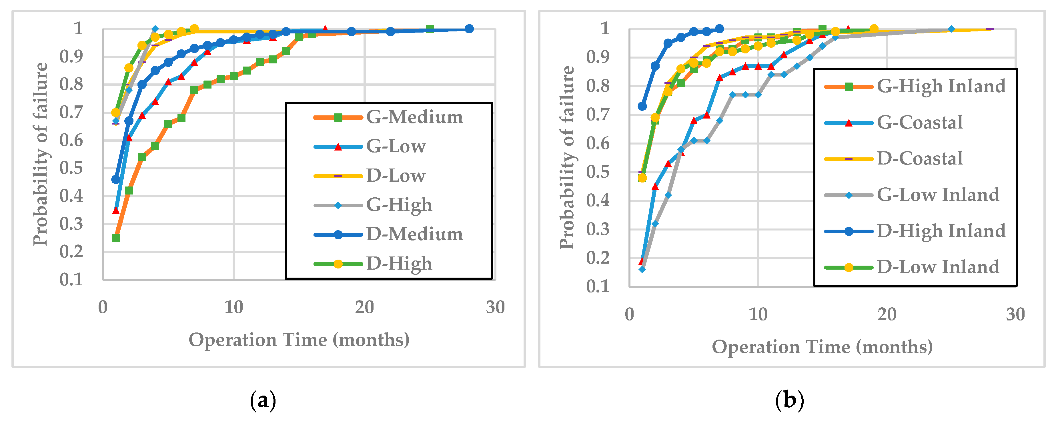
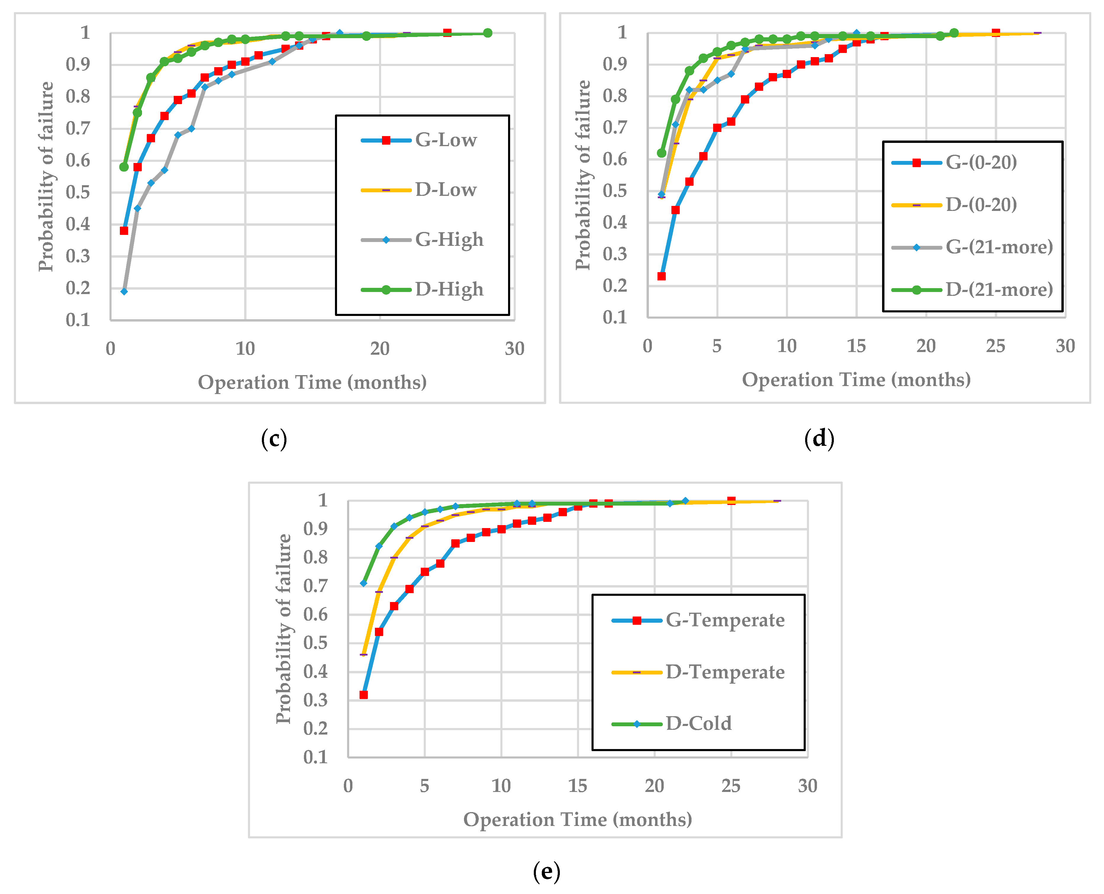
Failure probabilities for every month of operation are estimated by using Bayesian updating; results are shown in Figure 3. Failure probabilities vary depending on the operational and environmental condition of wind turbines. Figure 3a shows that geared-drive turbines with medium capacity factor have the lowest probability of failures for most of the time, while direct-drive turbines with high capacity factor have the highest probabilities of failures. Geared-drive turbines at low inland locations have the lowest probability of failure while direct-drive high inland turbines have the highest probability of failures as can be seen in Figure 3b. In the first three month of operation only 40% of the failures occurred for low inland geared-drive turbines while 95% of the failures occurred for direct-drive high inland turbines. Figure 3c shows that geared-drive wind turbines at high MAWS locations have the lowest probability of failures whereas direct-drive turbines regardless of their mean annual wind speed they have the highest probability of failures at every month of operation. Geared-drive wind turbines with low number of previous failures have the lowest probability of failures whereas direct-drive turbines with high number of failures have the highest probability of failures as seen in Figure 3d. It is seen on Figure 3e that geared-drive at temperate climates have the lowest probability of failure comparing to direct-drive turbines in both temperate and cold regions. It is also seen from Figure 3e that direct-drive turbines in cold climatic regions have higher probability of failures comparing to the ones in temperate-climates. Overall, direct drive wind turbines with high capacity factor at high inland, high mean annual wind speed at cold regions with high number of previous failures have a greater monthly probability of failures.

5.2. Time-to-Repair Probabilities by Bayesian Updating

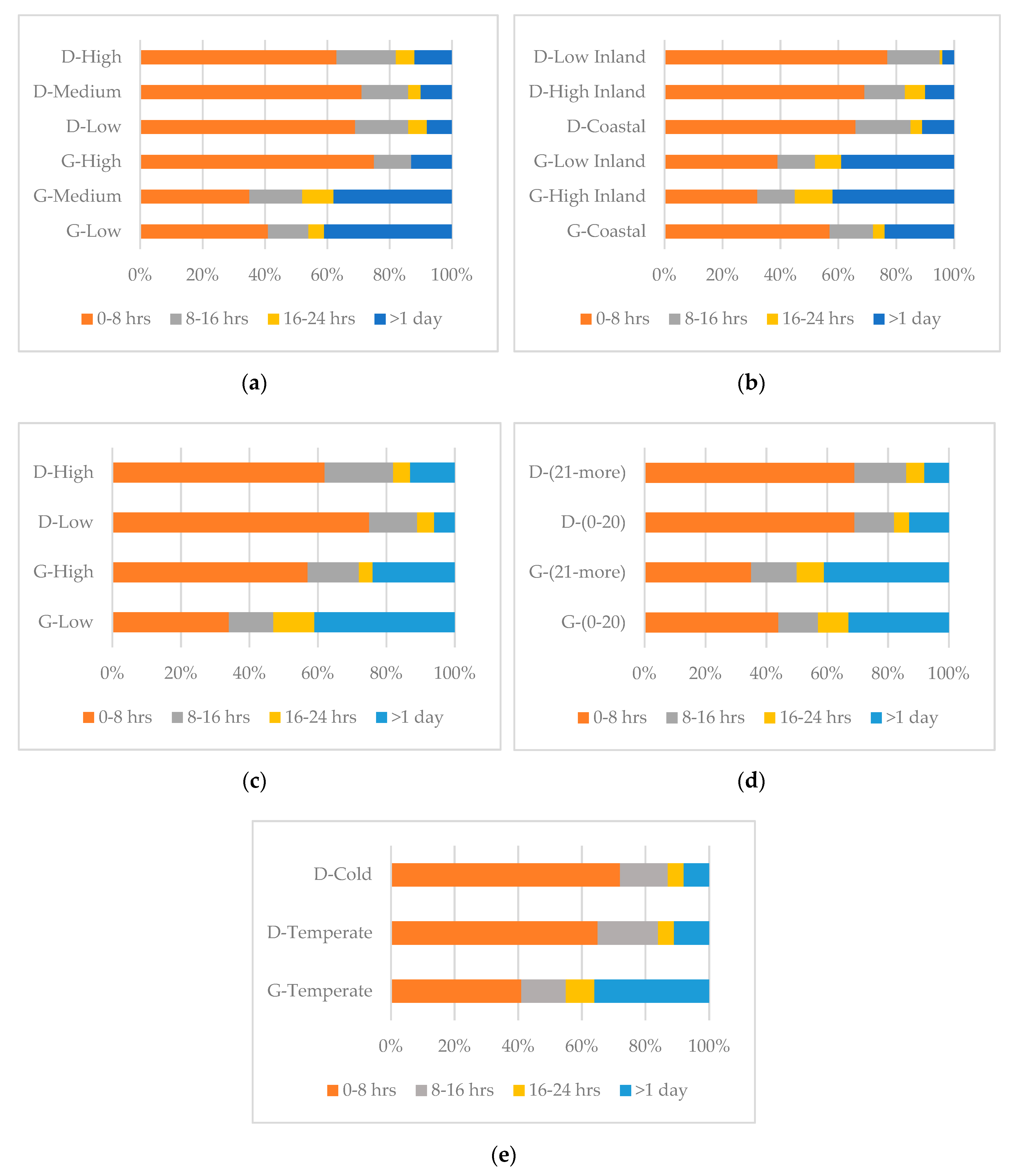
Bayesian updating results are shown in Figure 4 for time-to-repair probabilities based on turbine design type and other environmental and operational conditions. Figure 4a shows the results of time-to-repair probabilities as a function of wind turbine capacity factors of. From these results, it is inferred that direct-drive turbines with high capacity factor have the highest probability of quick repairs and the lowest probability of delayed repairs, whereas geared-drive turbines with medium capacity factor have the lowest probability of quick repairs and highest probability of delayed repairs. It is also shown in Figure 4a that geared-drive turbines with high capacity factor have the highest probability of quick repairs in geared-drive turbines. Figure 4b shows that direct-drive turbines at low inland locations have the lowest probability of delayed repairs such that 96% of the failures are repaired in less than one day. On the other hand, geared-drive turbines at high inland locations have the highest probability of delayed repairs such that 42% of the failures is repaired in more than one day. Figure 4c shows that there is not a common pattern for TTR probabilities of different design types of wind turbines based on mean annual wind speed. Direct-drive turbines at low MAWS locations have the highest probability of quick repairs and lowest probability of delayed repairs, contrarily, geared-drive turbines at low MAWS locations have the highest probability of delayed repairs and lowest probability of quick repairs. Figure 4d shows that number of previous failures do not change the share of probability of TTR values significantly for direct-drive wind turbines. However, geared-drive turbines which have less than 20 failures have 44% of time-to-repair in less than 8 h, whereas geared-drive turbines which have more than 20-failures history have 65% of time-to-repair in more than 8 h. It is observed from Figure 4e that there is a slight impact of temperate climate on time-to-repair for direct-drive turbines. In temperate climates, direct-drive wind turbines have lower share of quick repairs and higher share of delayed repairs comparing to cold climates. Since there is no data from cold climates for geared-drive wind turbines the only comparison can be done against direct-drive wind turbines at temperate locations. It is seen from Figure 4e that geared-drive turbines in temperate climate have lower share of quick repairs and higher share of delayed repairs comparing to the direct-drive turbines at cold climates. Overall, geared-drive wind turbines with low capacity factor and high number of previous failures at high inland, low mean annual wind speed and temperate locations have a higher than on day probability of delayed repair time.

5.3. Predicting Cost of Failures

As discussed in Section 3, we used machine learning methods to predict times-to-failure (TTF) and times-to-repair (TTR).

Table 6. Comparison of prediction accuracies.

Method	Output	Prediction Accuracy	Overall Prediction Accuracy
LR	TTF	0.744	0.694
	TTR	0.643
ANN	TTF	0.742	0.697
	TTR	0.652
KNN	TTF	0.733	0.687
	TTR	0.641
SVM	TTF	0.741	0.686
	TTR	0.631

shows the TTF and TTR prediction accuracies obtained via machine learning from four methods, based on 10-fold cross validation.

A 10-fold cross validation showed that ANN has 74.2% prediction accuracy with a single hidden layer and eight neurons for TTF and 65.2% prediction accuracy for TTR classifications with a single hidden layer and nine neurons; these are deemed to be satisfactorily accurate [11]. For KNN applications, parameters are used as k = 100 and weighted distance with Euclidian distances. Since ANN is determined as giving the greatest overall accuracy, thus 69.7%, among all four techniques, TTF and TTR prediction results from ANN are integrated to predict wind turbine cost of failures depending on their operational and environmental conditions of wind turbines. All machine learning applications are done in an Orange machine learning toolbox [30]. The TTF and TTR probability matrices from the considered ANN models are presented in Appendix A. The following sections explain the results based on three different capacity factors.

5.3.1. Low Capacity Factor

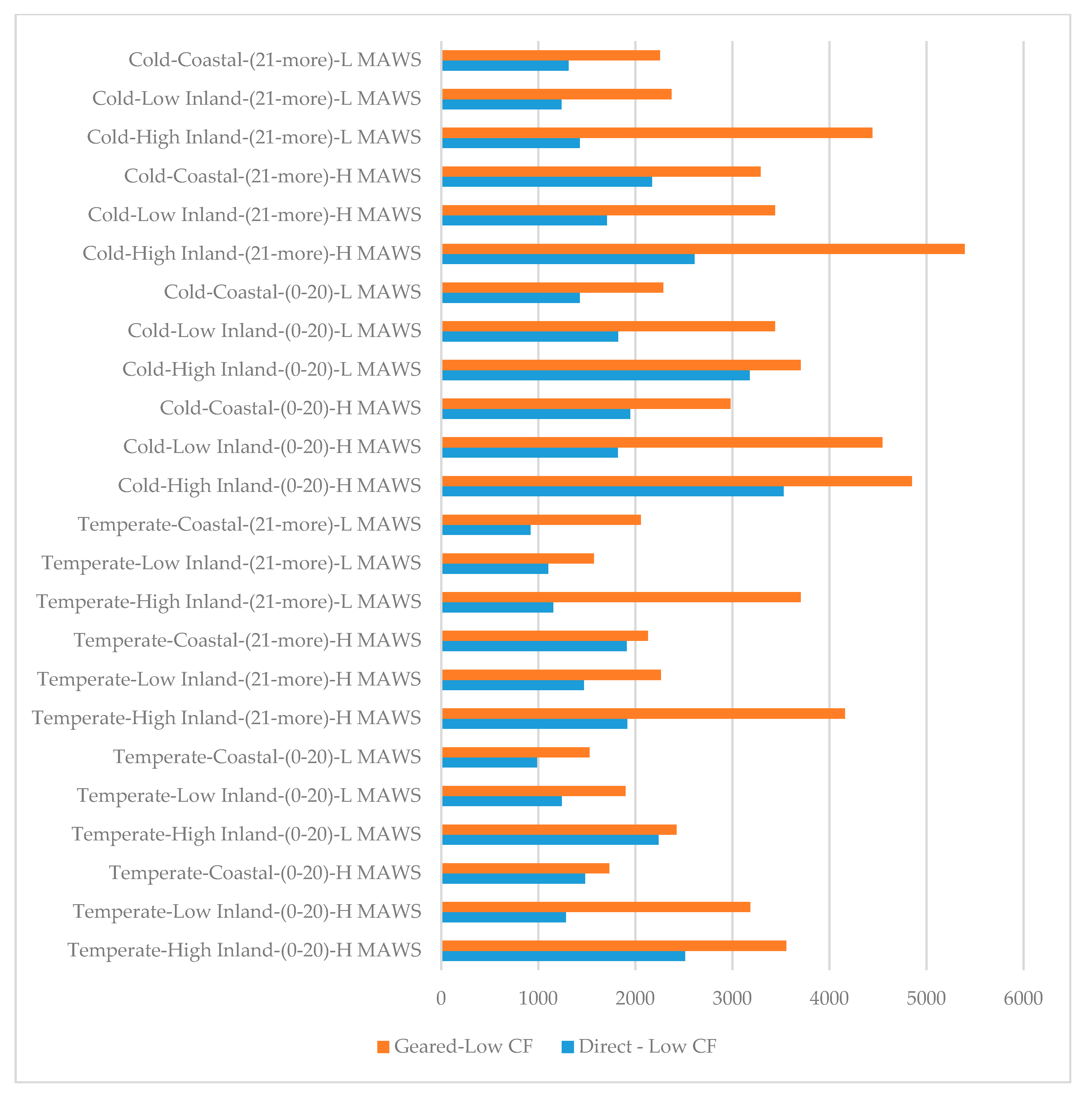
Figure 5 shows that geared-drive wind turbines operating at low capacity, have higher estimated costs at high inland locations than direct-drive turbines which operate at a low capacity factor. The highest distinction between the two types of turbines is noted at the high inland locations with low mean average wind speed (MAWS) regardless of their number of previous failures and climatic regions. This can be attributed to the increased numbers of start-stop events at low capacity factors as well as the potential increase of gust and time-to-access to the site for maintenance. In other words, geared-drive turbines would tend to have failures that result to more costs than direct-drive turbines Although there is no combination of factors that make geared-drive wind turbines more favorable, it is noted that temperate locations with coastal and low inland geography are the locations with the least distinction of cost of failure between direct-drive and geared-drive wind turbines. Overall, cold weather and high inland locations with higher MAWS direct-drive turbines exhibit lower repair-associated costs, whereas at temperate and coastal or low inland locations with lower MAWS geared-drive wind turbines are more favorable considering higher initial cost of direct-drive wind turbines.

5.3.2. Medium Capacity Factor

Figure 6 shows that at medium capacity factor locations the distinction between direct-drive and geared-drive turbines become closer. This can be attributed to the lower number of start-stop times where geared-drive turbines remain active with a medium energy production level comparing to the low-capacity factor areas. In other words, the wear and tear potential due to start-stop is reduced for geared-drive turbines at medium capacity factor in comparison with low-capacity factor locations. The highest distinction between the two types of wind turbines is noticed at high inland locations with higher NOPF and lower MAWS regardless of climatic region for the favor of direct-drive wind turbines. Geared-drive wind turbines become more favorable at temperate costal locations with higher MAWS regardless of number of previous failures with medium capacity factor. Overall, temperate and low inland or coastal locations are the most favorable locations for a geared-drive wind turbine considering higher initial cost of direct-drive wind turbines comparing to geared-drive wind turbines. This can be attributed to the shorter repair time and lower probability of failures of geared-drive wind turbines at medium capacity factor locations.

5.3.3. High Capacity Factor

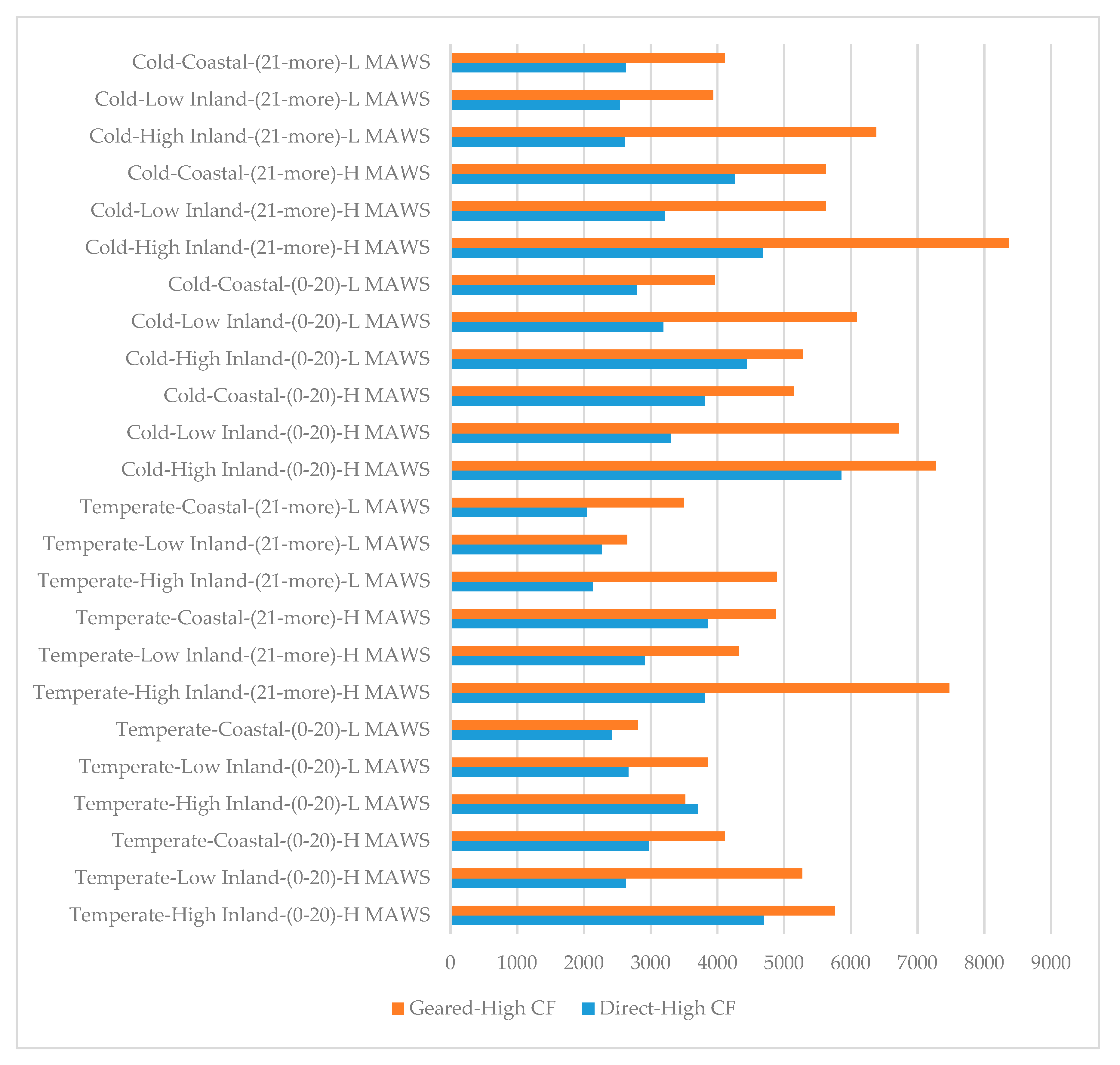
As shown in Figure 7, geared-drive turbines which operate with high capacity factor have higher estimated costs than direct-drive turbines which operate at a high capacity factor, regardless of geography, mean annual wind speed and previous failure history. The highest distinction between the two turbine designs is noted in high inland locations with the factors of higher number of previous failures and higher mean annual wind speed. This can be attributed to the fatigue of geared-drive wind turbines which would lead to higher probability of delayed repair-time at high capacity factor locations. On the other hand, on a temperate high inland location with low MAWS and low NOPF geared-drive turbines become more favorable in terms of failure costs. The cost of failure for direct drive wind turbines are generally the most favorable (repair cost wise) at coastal and low inland locations and the least favorable on high inland locations regardless of the other risk factors. This can be attributed to more steady wind regime and lower gust probability at coastal and low inland locations. However, for geared-drive wind turbines, low inland locations become unfavorable over high inland locations in cases of low NOPF and low MAWS, although high inland locations are generally the least favorable.

6. Conclusions

This study presents applications of two reliability prediction approaches: The first is Bayesian updating for wind turbine failure probability and repair time estimation based on wind turbine design type and environmental and operational conditions. The second approach is prediction of cost of failures for wind turbines based on combinations of environmental and operational factors, using machine learning methods. This study culminated to a decision support tool for wind farm operators to predict cost of failures from wind turbines based on environmental and operation conditions. Consequently, the tool can guide investment decisions associated with specific sites and wind turbine types. Furthermore, this tool can be utilized for decision-making in accepting or rejecting a third-party service provider’s O&M contract offers. The following conclusions are drawn from this study:

• Time-to-failure and time-to-repair values for wind turbines vary according to operational and environmental conditions.
• A high probability of failure is noted at the high inland locations for direct-drive turbines; a 73% probability of failure within the first month of operation is predicted. However, it should be noted that 69% of the failures for direct-drive turbines at high inland locations are fixed in less than 8 h.
• Higher probability of delayed repairs (more than 1 day) is noted at high inland locations for geared-drive turbine types with medium capacity factor and high number of previous failures.
• Geared drive turbines have greater expected cost of failures at high inland and high capacity factor locations that increase the cost of failure differences between geared and direct drive turbines, except for the temperate climates.
• High inland locations increase both probability of failures and probability of delayed time-to-repair.
• Medium capacity factor (20 ≤ CF ≤ 40%) lowers failure frequency, but increases delayed time-to-repair probability for geared-drive wind turbines.
• Direct-drive turbines are more favorable (have lower costs associated with repairs and unavailability) for locations with high capacity factor (more than 40%) and low capacity factor (less than 20%) whereas geared-drive turbines are shown to have lower repair and failure costs at temperate-coastal locations with medium capacity factor (between 20% and 40%) and high mean annual wind speed (MAWS).

To the authors’ knowledge, this is the first application of Bayesian updating for predicting wind turbine failures and time-to-repair in conjunction to wind turbine failure cost estimation using artificial neural network. This study collaborated previous studies that show an increase of failure probability associated high elevation and high capacity factors [4,8]. Additional studies can involve the following: (a) Up-to-date repair costs. The costs of time-to-repair are assumed to be fixed for geared and direct-drive wind turbines; however, the material costs might differ in different wind turbine types, and if those are known, the associated values should be introduced in the decision tool. (b) Our study involves wind turbines which have at most 14 years of operation, and it does not specifically consider a potential wear-out phase towards the last years of a wind turbine lifetime. Therefore, more detailed time-to-failure and cost for time-to-repair estimations are needed. (c) Future studies should also gather and investigate data from wind turbine reliability in more distinct climatic conditions and additional wind turbine types, than those included in the WMEP database.

References

1. Mone, C.; Hand, M.; Bolinger, M.; Rand, J.; Heimiller, D.; Ho, J. 2015 Cost of Wind Energy Review; National Renewable Energy Lab. (NREL): Golden, CO, USA, 2017. [CrossRef]
2. Besnard, F. On Optimal Maintenance Management for Wind Power Systems. DIVA, 2009. Available online: http://urn.kb.se/resolve?urn=urn:nbn:se:kth:diva-11793 (accessed on 5 January 2019).
3. Ortegon, K.; Nies, L.F.; Sutherland, J.W. The Impact of Maintenance and Technology Change on Remanufacturing as a Recovery Alternative for Used Wind Turbines. Procedia Cirp 21st Cirp Conf. Life Cycle Eng. 2014, 15, 182–188. [Google Scholar] [CrossRef] [Green Version]
4. Faulstich, S.; Hahn, B.; Tavner, P.J. Wind Turbine Downtime and Its Importance for Offshore Deployment. Wind Energy 2011, 14, 327–337. [Google Scholar] [CrossRef]
5. Wilson, G.; McMillan, D. Assessing Wind Farm Reliability Using Weather Dependent Failure Rates. J. Phys. Conf. Ser. 2014, 524, 012181. [Google Scholar] [CrossRef] [Green Version]
6. Slimacek, V.; Lindqvist, B.H. Reliability of Wind Turbines Modeled by a Poisson Process with Covariates, Unobserved Heterogeneity and Seasonality. Wind Energy 2016, 19, 1991–2002. [Google Scholar] [CrossRef]
7. Reder, M.; Yürüşen, N.Y.; Melero, J.J. Data-Driven Learning Framework for Associating Weather Conditions and Wind Turbine Failures. Reliab. Eng. Syst. Saf. 2018, 169, 554–569. [Google Scholar] [CrossRef] [Green Version]
8. Reder, M.; Melero, J.J. A Bayesian Approach for Predicting Wind Turbine Failures Based on Meteorological Conditions. J. Phys. Conf. Ser. 2018, 1037, 062003. [Google Scholar] [CrossRef] [Green Version]
9. Leigh, J.M.; Dunnett, S.J. Use of Petri Nets to Model the Maintenance of Wind Turbines. Qual. Reliab. Eng. Int. 2016, 32, 167–180. [Google Scholar] [CrossRef] [Green Version]
10. Carlos, S.; Sánchez, A.; Martorell, S.; Marton, I. Public Key Services and Infrastructures EUROPKI-2010-Mathematical Modelling in Engineering & Human Behaviour 2011. Math. Comput. Model. 2013, 57, 1884–1890. [Google Scholar] [CrossRef]
11. Kerres, B.; Fischer, K.; Madlener, R. Economic Evaluation of Maintenance Strategies for Wind Turbines: A Stochastic Analysis; SSRN Scholarly Paper Social Science Research Network, 1 March 2014; Rochester: New York, NY, USA, 2014; Available online: https://papers.ssrn.com/abstract=2469795 (accessed on 5 January 2019).
12. Raza, A.; Ulansky, V. Optimal Preventive Maintenance of Wind Turbine Components with Imperfect Continuous Condition Monitoring. Energies 2019, 12, 3801. [Google Scholar] [CrossRef] [Green Version]
13. Ozturk, S.; Fthenakis, V.; Faulstich, S. Failure Modes, Effects and Criticality Analysis for Wind Turbines Considering Climatic Regions and Comparing Geared and Direct Drive Wind Turbines. Energies 2018, 11, 2317. [Google Scholar] [CrossRef]
14. Ozturk, S.; Fthenakis, V.; Faulstich, S. Assessing the Factors Impacting on the Reliability of Wind Turbines via Survival Analysis—A Case Study. Energies 2018, 11, 3034. [Google Scholar] [CrossRef] [Green Version]
15. Arcos Jiménez, A.; Gómez Muñoz, C.Q.; García Márquez, F.P. Machine Learning for Wind Turbine Blades Maintenance Management. Energies 2018, 11, 13. [Google Scholar] [CrossRef] [Green Version]
16. Elasha, F.; Shanbr, S.; Li, X.; Mba, D. Prognosis of a Wind Turbine Gearbox Bearing Using Supervised Machine Learning. Sensors 2019, 19, 3092. [Google Scholar] [CrossRef] [PubMed] [Green Version]
17. Zhang, L.; Liu, K.; Wang, Y.; Omariba, Z.B. Ice Detection Model of Wind Turbine Blades Based on Random Forest Classifier. Energies 2018, 11, 2548. [Google Scholar] [CrossRef] [Green Version]
18. Lu, Y.; Madanat, S. Bayesian Updating of Infrastructure Deterioration Models. Transp. Res. Rec. 1994, 15, 110–114. [Google Scholar]
19. Ghonima, O. Statistical Modeling of United States Highway Concrete Bridge Decks. Thesis, University of Delaware, 2017. Available online: http://udspace.udel.edu/handle/19716/23068 (accessed on 23 December 2018).
20. Asri, H.; Mousannif, H.; Moatassime, H.A.; Noel, T. Using Machine Learning Algorithms for Breast Cancer Risk Prediction and Diagnosis. Procedia Comput. Sci. 2016, 83, 1064–1069. [Google Scholar] [CrossRef] [Green Version]
21. Kotsiantis, S.; Pierrakeas, C.; Pintelas, P. Predicting Students’ Performance in Distance Learning Using Machine Learning Techniques. Appl. Artif. Intell. 2004, 18, 411–426. [Google Scholar] [CrossRef]
22. Global Wind Atlas. Available online: https://globalwindatlas.info/ (accessed on 26 June 2018).
23. Peel, M.; Finlayson, B.; Mcmahon, T. Updated World Map of the Koppen-Geiger Climate Classification. Hydrol. Earth Syst. Sci. 2007, 11, 1633–1644. [Google Scholar] [CrossRef] [Green Version]
24. Kruschke, J.K. Doing Bayesian Data Analysis: A Tutorial with R and BUGS, 1st ed.; Academic Press, Inc.: Orlando, FL, USA, 2010. [Google Scholar]
25. Keisan Online Calculator. Retrieved January 10, 2019. Available online: https://keisan.casio.com/ (accessed on 23 December 2018).
26. Patterson, J.; Gibson, A. Deep Learning. Available online: http://shop.oreilly.com/product/0636920035343.do (accessed on 27 December 2018).
27. Li, C.; Zhang, S.; Zhang, H.; Pang, L.; Lam, K.; Hui, C.; Zhang, S. Using the K-Nearest Neighbor Algorithm for the Classification of Lymph Node Metastasis in Gastric Cancer. Comput. Math. Methods Med. 2012. [Google Scholar] [CrossRef] [Green Version]
28. Bhondve, A.T.; Bhame, V.S.; Kadam, A.R.; Kopnar, K.D. Breast cancer disease prediction: Using machine learning. Int. Res. J. Eng. Technol. 2019, 6, 428. [Google Scholar]
29. Ahmed, K.A.; Aljahdali, S.; Hundewale, N.; Ahmed, K.I. Cancer Disease Prediction with Support Vector Machine and Random Forest Classification Techniques. In Proceedings of the 2012 IEEE International Conference on Computational Intelligence and Cybernetics (CyberneticsCom), Bali, Indonesia, 12–14 July 2012; pp. 16–19. [Google Scholar]
30. Demsar, J.; Curk, T.; Erjavec, A.; Gorup, C.; Hocevar, T.; Milutinovic, M.; Mozina, M.; Polajnar, M.; Toplak, M.; Staric, A.; et al. Orange: Data Mining Toolbox in Python. J. Mach. Learn. Res. 2013, 14, 2349–2353. [Google Scholar]
31. ISET. Windenergie Report Deutschland 2006; Fraunhofer: Munich, Germany, 2016. [Google Scholar]
Figure 1. Feed-forward multilayer neural network [26].
Energies 13 01149 g001
Figure 2. Schematic of developing the decision support tool to predict cost of failures for wind turbines; TTF: time-to-failure; TTR: time-to-repair.
Energies 13 01149 g002
Figure 3. Time-to-failure of wind turbines based on operational and environmental factors. (a) Capacity factor, (b) geography, (c) mean annual wind speed, (d) number of previous failures, (e) climatic region. (The en dashes here and in the Figure 4, Figure 5, Figure 6 and Figure 7 mean “with” the other condition(s) except for the numbering ranges for NOPF.)
Energies 13 01149 g003aEnergies 13 01149 g003b
Figure 4. Time-to-repair of wind turbines based on operational and environmental factors. (a) capacity factor (b) geography (c) mean annual wind speed (d) number of previous failures (e) climatic regions.
Energies 13 01149 g004
Figure 5. Predicted cost of failures at locations with low capacity factor.
Energies 13 01149 g005
Figure 6. Predicted cost of failures at locations with medium capacity factor.
Energies 13 01149 g006
Figure 7. Predicted cost of failures at locations with high capacity factor.
Energies 13 01149 g007