Active Shock Absorber Control Based on Time-Delay Neural Network

Abstract

A controlled suspension usually consists of a high-level and a low-level controller. The purpose the high-level controller is to analyze external data on vehicle conditions and make decisions on the required value of the force on the shock absorber rod, while the purpose of the low-level controller is to ensure the implementation of the desired force value by controlling the actuators. Many works have focused on the design of high-level controllers of active suspensions, in which it is considered that the shock absorber can instantly and absolutely accurately implement a given control input. However, active shock absorbers are complex systems that have hysteresis. In addition, electro-pneumatic and hydraulic elements are often used in the design, which have a long response time and often low accuracy. The application of methods of control theory in such systems is often difficult due to the complexity of constructing their mathematical models. In this article, the authors propose an effective low-level controller for an active shock absorber based on a time-delay neural network. Neural networks in this case show good learning ability. The low-level controller is implemented in a simplified suspension model and the simulation results are presented for a number of typical cases.

1. Introduction

The existing vehicle suspension systems can be divided into three categories: passive, adaptive or semi-active, and active [1,2].

Passive suspensions are completely dissipative systems in which the energy of motion of the unsprung mass is transformed into thermal energy. In such structures, the shock absorber performance is predetermined at the stage of suspension design, and cannot be changed further. Adaptive or semi-active suspensions are also dissipative systems. However, in such designs, the performance of the shock absorber can be changed during vehicle movement in accordance with the objectives of the control system. Some authors do not distinguish the terms “adaptive” and “semi-active” suspension, while others notice the difference in operating frequencies [1]. Further in the article the term “semi-active shock absorber” is proposed. These designs can only limit the movement of the sprung mass. For the problem of fully stabilizing the mass in a given position, active suspension should be used [3].

Active shock absorbers are equipped with an external source of energy so that these systems can generate forces on the rod, regardless of the unsprung mass displacement. The dissipative characteristics of passive, semi-active, and active shock absorbers are presented in their general forms in Figure 1a–c, respectively. The following notation is used in the figure: F—force on the shock absorber rod, N; v—rod movement velocity, m/s. As can be seen in Figure 1b, the set of dissipative characteristics of a semi-active shock absorber lies in I and III quadrants; thus, the force vector F is always in one direction with the velocity vector v.

In an active shock absorber, the set of dissipative characteristics cover all IV quadrants due to an external energy source, and force and velocity vectors can be oppositely directed. This property is the great advantage of active shock absorbers, and it allows, in theory, the achievement of a complete absence of movement of the vehicle body for the given planes.

Presently, among controlled suspension systems, designs of semi-active shock absorbers are the most widely spread on the market [4,5,6]. This is largely due to their minimal energy requirements. These are dissipative devices for which input power is needed only to control the valves [6]. One of the classes of such devices are the shock absorbers with the possibility of stepwise changes in working characteristics. Servomotors are generally used in this design, the following works on such shock absorbers are most notable: [7,8,9]. Solenoid valves are also often used in the construction of shock absorbers [8,9,10,11,12,13,14]. The next step in the development of semi-active shock absorbers is the usage of valves that allow dissipative characteristics to change continuously [15,16].

Active suspensions have not received wide commercial distribution until recently. The main reasons for this are their extremely high power consumption requirements. Concepts [17,18,19,20,21], as well as research work on the control of active suspension systems [21,22,23,24,25,26,27,28,29], can be found in the literature. There have also been a few approaches to the design of high-level controllers for active suspension that have dealt with the delays and failures of actuators [30,31]. On the other hand, current trends in the development of vehicles with increased supply voltage, as well as improvements in the design of external energy sources, have allowed the creation of promising new solutions for active shock absorbers.

As noted in [2], a big disadvantage of existing low-level controllers of active and semi-active shock absorbers is their usage of idealized dynamical models. A large number of mass-produced controllers based on dissipative characteristics have been provided in the form of lookup tables. However, this approach does not ensure the high accuracy of the control system, since it does not take into account the dynamics of actuators. Moreover, the performance of the shock absorber has a strong hysteresis property, with origin loops that are asymmetrical to the coordinates (Figure 2 and Figure 3). Recently, there have been works in which authors have modeled real dissipative characteristics and develop control algorithms. In papers [32,33,34,35,36,37], approaches have been considered that model the hysteresis property of the shock absorber; however, the dissipative characteristic is assumed to be symmetrical.

One of the promising modern approaches to shock absorber controller design is the development of algorithms based on the use of artificial neural networks (NNs). Among all the numerous topologies, time delay neural networks (TDNNs) are noticeable. TDNNs were first introduced in [38]. The following works represent the results of the successful implementation of time delay neural networks in the design of magnetorheological damper controllers [39,40,41,42,43].

The objective of the article is to design a low-level controller for a fully active shock absorber with asymmetric hysteresis loops of dissipative characteristics, and to test its effectiveness on an existing vehicle model. Active shock absorbers have two types of control inputs: currents on electromagnetic valves and hydraulic pump flow rate. The proposed controller is based on a neural network with a time delay. The resulting control system can then be used to control a real shock absorber. In view of the parameters of the studied shock absorbers, developed control system is assumed to be used for passenger vehicles. However, the proposed approach is universal, and can be applied to design controllers for the shock absorbers of various vehicles (e.g., trucks, motorcycles, etc.). This article is organized as follows: the methodology is described in Section 2; Section 3 describes the active damper used for controller design and deals with designing neural networks, training, and proposed controller architecture; Section 4 describes the simulation results; in Section 5, the developed controller is implemented into a quarter vehicle suspension model. Finally, the obtained conclusions are discussed.

2. Methodology

The procedure of this research is as follows: first, experimental dissipative characteristics of the active shock absorber were obtained for different control inputs. Next, the training dataset was collected. The neural network was then trained using the dataset. The structure of the neural network, inputs, and outputs, and the number of layers, as well as the number of neurons in each layer, were selected by trial and error. To design a low-level controller, it was proposed to use a neural network with 3 Proportional-Integral-Derivative PID controllers. The controller then was tested on different reference signals. To test the effectiveness of the low-level controller, it was implemented in a quarter vehicle model. NN training and simulation were performed in Matlab R2016b. Trained NN, as well as the training dataset, are attached to the paper.

3. Time Delay Neural Network Controller Design

3.1. Active Shock Absorber Description

The fully active shock absorber has two types of input control signals:

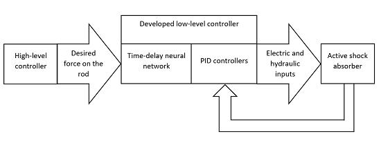
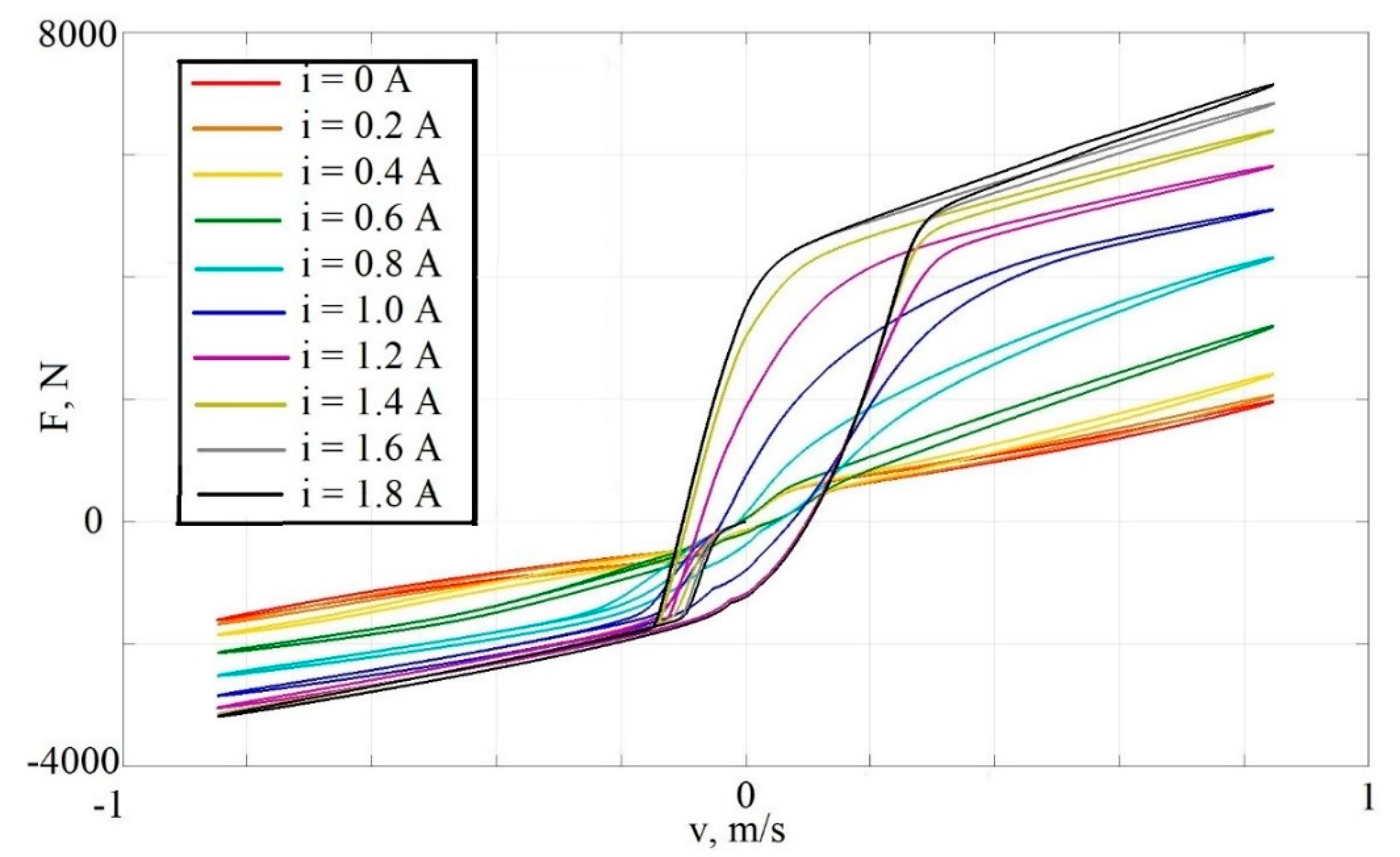
• The currents on the solenoid valves of the compression and rebound strokes $i_C,i_R$, whose values lie in the range 0…1.8 A. Applying the current value to the valve changes its capacity. The values of the force on the shock absorber rod and the values of the speed of the rod always have the same sign. Thus, a shock absorber controlled only by the currents on the valves works as semi-active. The set of a dynamic dissipative characteristics of the shock absorber for different values of currents is shown in Figure 2. In Figure 2 and Figure 3, the following notation in used: $F—$ force on the rod, $v$—velocity of the rod, $i$—control current, $Q$—hydraulic pump flow rate.
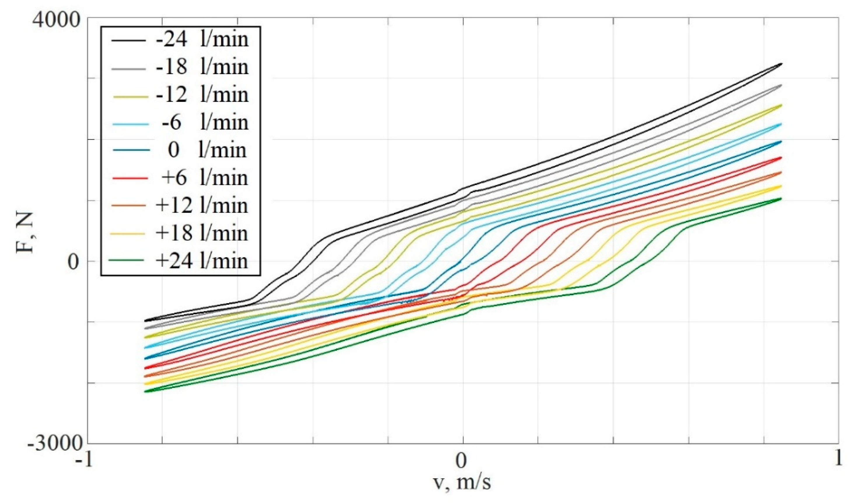
• The hydraulic pump flow rate Q lies in the range of −24…24 l/min, where the sign determines the direction of the fluid flow. The set of dissipative characteristics obtained for different values of Q are presented in Figure 3. A pump is essentially an external source of energy in the system, and thus it becomes possible to generate forces on the rod opposite to the direction of the movement of the rod. This is how the “active” property of the shock absorber is realized.

As can be seen from Figure 2 and Figure 3, the dynamic dissipative characteristics are substantially nonlinear. In addition, the hysteresis property can be seen in the system. It is also important to note the asymmetry of the hysteresis loops relative to the origin of coordinates. Thus, to develop an efficient and accurate control system, it is mandatory to take into account not only the instantaneous values of the states of the dynamic system, but their time series.

.

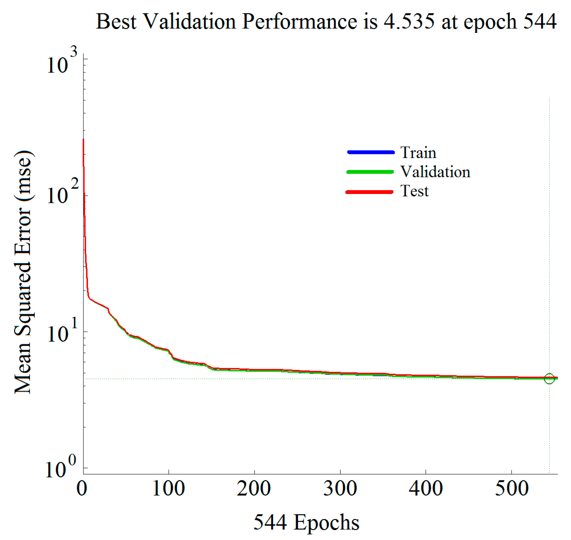
3.2. Neural Network Training

An artificial time-delayed neural network is in principle an extension of a multi-layer perceptron that allows time sequences to be taken into account to work with problems in which the signals are functions of time and previous values. In this case, the neurons had an interesting property of memorizing the sequence of values of the input signals. This property also made it possible to train NNs to approximate dynamic systems with hysteresis. A schematic diagram of the TDNN with $n$ time delays and $m$ hidden layers is presented in Figure 4.

In the learning process, the backpropagation algorithm is usually used; accordingly, all methods for accelerating backpropagation can be applied.

For the best results, the training sample of the neural network should cover as much of the working range of the system states as possible. To form a training dataset, the simulation was performed for 40 s. In this case, the inputs on the system were as follows:

• Displacement of the shock absorber rod $x$ was defined as the product of two chirp signals, with a frequency varying from 0.01 to 2 Hz, and from 1 to 4 Hz. The gain of the multiplication is 0.03 m.
• The velocity of movement of the rod $v$ was defined as the time derivative of the displacement.
• Electrical currents and volumetric flow rate of a hydraulic pump were also defined as the product of two chirp signals, with frequencies variable for $i_R$ from 1 to 1.2 Hz, for $i_C$ from 1 to 1.3 Hz, and for $Q$ from 1 to 1.3 Hz, with amplitudes in the range of their possible values.

The output of the system was the force on the shock absorber rod. Training sample signals are presented in Figure 5.

There are no universal methods for choosing the NN topology, its training algorithm, and its parameters. Known patterns are mainly obtained empirically and are advisory in nature. By trial and error, the following was defined:

TDNN input

$$q=\left(x, x^{-1}, x^{-2}, v, v^{-1}, v^{-2}, F, F^{-1}, F^{-2}\right),$$

(1)

where $x$ is rod movement, $v is$ rod velocity, and $F$ is force on the rod, as well as their time delays up to the second step. Thus, the input layer of the neural network consisted of nine neurons. For the output layer of the neural network, we choose three neurons corresponding to the control signals; then, the output of the neural network could be written as a vector.

$$y=\left(i_{R_{NN}}, i_{C_{NN}}, Q_{NN}\right).$$

(2)

The network structure was then written as 9-20-10-3, so that it had nine input layer neurons, two hidden layers (with 20 and 10 neurons, respectively), and three neurons in the output layer. Sigmoid function was chosen as an activation function for neurons in the hidden layers and linear function for output layer neurons.

The training process diagram is shown in Figure 6.

The following parameters were chosen for the training process:

• Algorithm: Levenberg-Marquardt backpropagation
• NN performance criteria: mean squared error (MSE)
• Training epoch: 2000
• Maximum number of validation degradation checks: 10
• Data division: random, 60% for training, 20% for validation and 20% for testing

After 544 epochs, training stopped because 10 validation checks had been reached. The NN MSE performance is presented in Figure 7. The figure shows that with an increase in the number of training epochs, the MSE of the neural network decreased for all three phases (blue line for training, green for validation, and red for testing).

Figure 8 shows a histogram of errors with 20 bins. Similar to the previous dependency, blue, green, and red colors represent training, validation, and testing phases, respectively. It can be seen from the figure that the errors were distributed relative to zero.

The graph in Figure 9 shows a regression analysis between the outputs of the NN and the desired targets. The solid line represents the best fit linear regression line between outputs and targets. The dashed line represents the best results (i.e., when targets were equal to NN outputs). The $R$ value is an indication of the relationship between the outputs and targets, taking values from 0 to 1, where 0 means no linear relationship, and 1 means an exact linear relationship. The overall $R$ value was 0.95211, so a strong relationship can be concluded.

Analyzing the graphs presented here, as well as conducting simulation experiments, conclusions about the successful training of the neural network can be drawn.

3.3. Controller Design

After the training process, the neural network is able to act as a controller. It can be said that the resulting neural network is an inverse dynamic model of the shock absorber, since the input variables of the shock absorber were the output of the neural network and vice versa. However, when using only a neural network in the control system, acceptable results can’t be achieved, because there is no feedback in such a system. For a feedback circuit, it is proposed to use the developed neural network together with other controllers that could compensate for inaccuracies in the NN approximation. The control system in this article is built using PID controllers. The PID control law is simple, and using it alone is not enough to precisely control the active shock absorber. However, the control system based on PIDs with the developed neural network shows good results. The architecture of the proposed control system is presented in Figure 10.

Here, we introduce three PID controllers—$PI{D}_{i_C}$, $PI{D}_{i_R}$ and $PI{D}_Q$—to compensate for NN errors in compression, rebound valve currents, and the volumetric flow rate, respectively.

4. Simulation Results

The testing of the developed controller was carried out using several scenarios of a desired force on the rod, covering a wide range of possible tasks for an active shock absorber: wave with changing frequency, wave with initial time delay, sawtooth, and step signals.

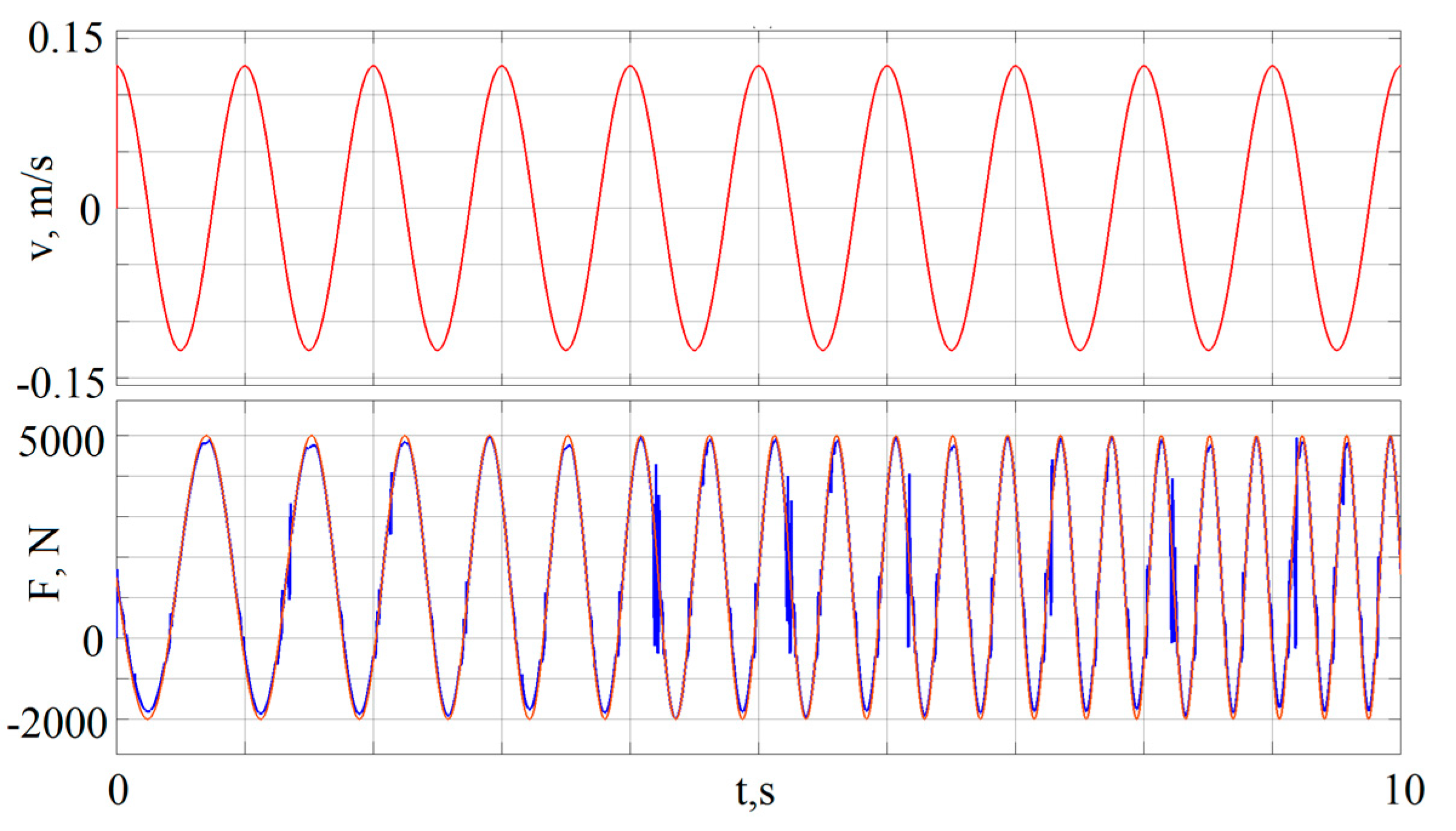
4.1. Providing the Desired Force in the Form of a Wave Signal with Increasing Frequency

One of the main tasks in controlling active suspension is to provide the desired force in the form of a wave. In this case, the frequency and phase of the wave can be arbitrary with respect to the input periodic effect on the rod. The simulation results were presented when the displacement of the shock absorber rod is in the form of $x=0.02\sin \left(2\pi ·2·t\right)$. In this case, we defined the desired value of the force to be specified as a chirp signal, with an amplitude increasing linearly from 1 to 3 Hz in 10 s. The gain of multiplication was 10,000. Since the dissipative characteristics were not symmetrical in the compression and rebound phases, the chirp signal was shifted up by 1500. The dependences obtained are shown in Figure 11. Discussions of the results are below.

4.2. Providing the Desired Force in the Form of a Wave Signal with Initial Time Delay

We selected the input of the shock absorber rod as in the previous scenario, but the frequency was increased to 1.5 Hz. The desired output value of the force on the rod was set as a wave signal with a frequency of 1 Hz and an initial delay of 1 s. The value of the force on the rod was equal to 1000 N. The results are shown in Figure 12.

4.3. Providing the Desired Force in the Form of a Sawtooth Signal

Next we considered the implementation of the output value of the system in the form of a sawtooth function. The input was the same as in the previous example. The results are presented in Figure 13. The maximum values of the error in the sawtooth rose sharply to the 15% limit, and the error stabilized around 0 in a short time (about 0.02 s).

4.4. Providing the Desired Force in the Form of a Step Signal

The step signal was considered, since it can be used to draw conclusions about the performance and accuracy of the control system in extreme scenarios of an instant change and in maintaining constant value of the outputs. The signal levels were -1000 and 4000 N. Step time was 1 s. Results are shown in Figure 14.

5. Implementation of the Developed Controller in the Quarter Vehicle Model

To test the efficiency of the developed controller, a simulation of a quarter-mass model of the vehicle was also carried out. The mass of the body was denoted by $m_b$, and the mass of the wheel by $m_w$. We denoted the vertical displacements of the body and the wheel as $x_b, x_w$, respectively. The road profile was set as $x_r$. For demonstration purposes, a simple model was used, where the operating characteristics of elastic and dissipative elements are considered to be linear and denoted by the stiffness coefficient $k_s$ and the damping coefficient $c_s$, respectively. The tire damping properties were ignored. The elastic properties of the tire were expressed as a linear characteristic with the coefficient $k_t$. A sketch of the quarter vehicle model is presented in Figure 15. The parameters used in the simulation are listed in

Table 1. Quarter vehicle suspension parameters.

Parameter	Symbol	Value (Unit)
Mass of the body	$m_b$	375 (kg)
Mass of the wheel	$m_w$	29.5 (kg)
Suspension stiffness	$k_s$	20.58 (kN/m)
Damping coefficient	$c_s$	772 (Ns/m)
Tire stiffness	$k_t$	200 (kN/m)

.

The force generated by the active shock absorber is $f_d$. Using Newton’s Second Law, we get [44]:

$$\begin{gathered} m_b{\ddot{x}}_b+k_s\left(x_b-x_w\right)+c_s\left({\dot{x}}_b-{\dot{x}}_w\right)+f_a=0, \\ {m}_w{\ddot{x}}_w-k_s\left(x_b-x_w\right)-c_s\left({\dot{x}}_b-{\dot{x}}_w\right)+k_t\left(x_w-x_r\right)-f_a=0. \end{gathered}$$

(3)

After corresponding transformations, the state space model is obtained:

$$\begin{gathered} \dot{x}=Ax+B{f}_d+Dx, \\ A={\left(\begin{array}{cccc}0& 0& 1& 0\\ 0& 0& 0& 1\\ -\raisebox{1ex}{$k_s$}\!\left/ \!\raisebox{-1ex}{$m_b$}\right.& \raisebox{1ex}{$k_s$}\!\left/ \!\raisebox{-1ex}{$m_b$}\right.& -\raisebox{1ex}{$c_s$}\!\left/ \!\raisebox{-1ex}{$m_b$}\right.& \raisebox{1ex}{$c_s$}\!\left/ \!\raisebox{-1ex}{$m_b$}\right.\\ \raisebox{1ex}{$k_s$}\!\left/ \!\raisebox{-1ex}{$m_w$}\right.& -\raisebox{1ex}{$\left(k_s+k_t\right)$}\!\left/ \!\raisebox{-1ex}{$m_b$}\right.& \raisebox{1ex}{$c_s$}\!\left/ \!\raisebox{-1ex}{$m_w$}\right.& -\raisebox{1ex}{$c$}\!\left/ \!\raisebox{-1ex}{$m_w$}\right.\end{array}\right)}^T, \\ B={\left( 0 , 0, -\raisebox{1ex}{$1$}\!\left/ \!\raisebox{-1ex}{$m_b$}\right., \raisebox{1ex}{$1$}\!\left/ \!\raisebox{-1ex}{$m_w$}\right. \right)}^T, \\ D={\left(0, 0, 0, \raisebox{1ex}{$k_t$}\!\left/ \!\raisebox{-1ex}{$m_w$}\right.\right)}^T, \\ x={\left(x_b, x_w, {\dot{x}}_b, {\dot{x}}_w\right)}^T. \end{gathered}$$

(4)

PID control gains are obtained in [34]. Controller output (desired force on the rod):

$$\begin{gathered} u\left(t\right)=f_d=k_{p}e+k_i{{\displaystyle \int }}_0^{t}e\left(\tau \right)d\tau +k_d\frac{de}{dt}, \\ e=x_b-x_w, \end{gathered}$$

(5)

where $e$ is the control system error; and $k_p$, $k_i$, $k_d$ are the proportional, integral, and differential gains of the controller, respectively.

The driving of a car through a single road bump was chosen to determine the quality of the test scenario. The road profile was defined in accordance with [34]:

$$x_r=\{\begin{array}{c}a\left(1-\cos \left({\omega }_r\left[t-0.5\right]\right)\right), if 0.5\le t\le 0.5+\raisebox{1ex}{$d_b$}\!\left/ \!\raisebox{-1ex}{$V_c$}\right.\\ 0, otherwise.\end{array}$$

(6)

where $a$ is half the height of the bump, $d_b$ is the bump width, $V_c$ is the speed of the vehicle, and ${\omega }_r=\raisebox{1ex}{$2\pi V_c$}\!\left/ \!\raisebox{-1ex}{$d_b$}\right.$. The irregularity profile as a function of time is presented in Figure 16 (the parameters are as follow:$a$ = 0.035 m, $d_b$ = 0.8 m, $V_c$ = 0.856 m/s).

In Figure 17, graphs of the desired force (output of the PID controller, red line) and the actual force on the shock absorber rod (blue line) are presented. As can be seen from this figure, the developed controller of the active shock absorber provided, with an acceptable level of error, the realization of the desired force. Figure 18 depicts a graph of the vertical acceleration of the vehicle body ${\ddot{x}}_b$ with a passive shock absorber (red line), and an active shock absorber with a developed controller (blue line). The advantage of using active shock absorbers and the possibility of a significant reduction in the level of dynamic loads thus can be seen in Figure 18.

The second type of road input, normally used to analyze the behavior of a vehicle’s suspension, is a periodical excitation. In Figure 19, the results are presented for the sine wave excitation with a frequency of 4 Hz and an amplitude of 0.03 m.

By using the sinusoidal input for the quarter vehicle model, overall frequency responses can be obtained for different frequency ranges. It can be seen that in the case of a sinusoidal excitation, the designed controller also provided sufficient results. The error peaks were very short in time (less than 0.01 s).

6. Conclusions and Discussion

The article presents an approach to developing a a low-level active shock absorber controller based on the use of a time-delayed neural network.

Training a neural network does not require high-precision physical and mathematical models of the control object and identification of its parameters. Thus, for designing the controller, experimental data are required to form a training dataset.

After the training, the neural network showed a good ability to approximate the inverse model of the active shock absorber. Combining a neural network with traditional PID controllers allowed it to compensate for its learning errors. Various simulations were carried out to assess the performance of the proposed approach. The results can be considered satisfactory for technical tasks, with a maximal error that did not exceed 15% with a very short stabilization time (around 0.02 s).

The proposed low-level controller was integrated into the existing high-level active suspension controller.

The results show the possibility of using time-delay artificial neural networks for the design of low-level controllers for an active shock absorber. Various combinations of the number of hidden layers of the neural network, as well as the number of neurons of each layer, can reduce the resulting errors. In addition, the usage of advanced control algorithms, instead of PID controllers, also can improve control system performance.

References

1. Heißing, B.; Ersoy, M. Chassis Handbook: Fundamentals, Driving Dynamics, Components, Mechatronics, Perspectives; Vieweg+Teubner Verlag: Berlin, Germany, 2011. [Google Scholar]
2. Barton, D.C.; Fieldhouse, J.D. Automotive Chassis Engineering; Springer: New York, NY, USA, 2018. [Google Scholar]
3. Pellegrini, E. Model-Based Damper Control for Semi-Active Suspension Systems. Ph.D. Thesis, TU Munchen, München, Germany, 2012. [Google Scholar]
4. Causemann, P. Moderne Schwingungsdämpfung. Automob. Z. 2003, 11, 1070–1079. [Google Scholar] [CrossRef]
5. Jautze, M.; Bogner, A.; Eggendinger, J.; Rekewitz, G.; Stumm, A. Der neue BMW 7er:Das Verstelldämpfersystem Dynamische Dämpfer Control; Automobiltechnische Zeitschrift, ATZ extra; Springer: New York, NY, USA, 2008; pp. 100–103. [Google Scholar]
6. Schwarz, R.; Biesalki, A.; Schöpfel, A.; Stingls, H. Der Neue Audi Q5: Audi Drive Select; Automobiltechnische Zeitschrift, ATZ extra; Springer: New York, NY, USA, 2008; pp. 60–64. [Google Scholar]
7. Savaresi, S.M.; Poussot-Vassal, C.; Spelta, C.; Sename, O.; Dugard, L. Semi-Active Suspension Control Design for Vehicles; Elsevier Ltd.: Amsterdam, The Netherlands, 2010. [Google Scholar]
8. Heyer, G. Trends in Stoßdämpferentwicklung. In Federungs- und Dämpfungssysteme; Krettet, O., Ed.; Fortschritte der Fahrzeugtechnik—Vieweg: Berlin, Germany, 1992; pp. 233–260. [Google Scholar]
9. Reimpel, J.; Stoll, H. Fahrwerktechnik: Stoß- und Schwingungsdämpfer, 2nd ed.; Vogel Verlag: Würzburg, Germany, 1989. [Google Scholar]
10. Causemann, P. Kraftfahrzeugstoßdämpfer; Bibliothek der Technik: Berlin, Germany, 1999; Volume 185. [Google Scholar]
11. Spielmann, M. Elektronische Dämpfkraftregelung EDCC. In Elektronik im Kraftfahrzeugwesen—Steuerungs-, Regelungs-, und Kommunikationssysteme; Kontakt & Studium—expert Verlag: Berlin, Germany, 2002; pp. 8–14. [Google Scholar]
12. Aliukov, S.; Alyukov, A. Analysis of Methods of Solution of Differential Equations of Motion of Inertial Continuously Variable Transmissions; SAE Technical Paper, SAE World Congress Experience; WCX: Warrendale, PA, USA, 2017; Volume 2017. [Google Scholar]
13. Aliukov, S.; Keller, A.; Alyukov, A. On the question of mathematical model of an overrunning clutch. In Lecture Notes in Engineering and Computer Science; 2015 World Congress on Engineering; WCE: London, UK, 2015; Volume 2218. [Google Scholar]
14. Wallentowitz, H. Aktive Fahrwerkstechnik; Vieweg: Berlin, Germany, 1991. [Google Scholar]
15. Schiehlen, W.; Hanss, M.; Iroz, I. Robust design of road vehicle suspension using fuzzy methods. In Proceedings of the 24th Symposium of the International Association for Vehicle System Dynamics (IAVSD 2015), Graz, Austria, 17–21 August 2015. [Google Scholar]
16. Causemann, P.; Kutschem, T. CDC(Continuous Damping Control) Ausführungen mit integriertem oder extern ausgeführten Proportional—Dämpfer—Ventile—Eine Bewertung zweier unterschiedlicher Konzepte. In Reifen—Fahrwerk—Fahrbahn (VDI Berichte); VDI-Gesellschaft Fahrzeug- und Verkehrstechnik, VDI-Verlag: Berlin, Germay, 1997; pp. 135–153. [Google Scholar]
17. Jungbluth, T. Federungs- und Dämpfungsinnovationen von ThyssenKrupp Bilstein; Fachpresse-Mitteilung IAA PKW: Berlin, Germany, 2005. [Google Scholar]
18. Obinabo, E.C.; Ighodalo, O. The utilization of an electric field sensitive effect for vibration control of viscous isolating system. Res. J. Appl. Sci. Eng. Technol. 2011, 3, 153–158. [Google Scholar]
19. Bose Suspension System. Available online: http://bose.de/DE/de/index.jsp (accessed on 29 February 2020).
20. Brown, S.N. Active Vehicle Suspension System. Patent EP 1 440 826 B1, 23 December 2013. [Google Scholar]
21. Münster, M.; Mair, U.; Gilsdorf, H.J.; Thom, A.; Müller, C.; Hippe, M.; Hoffmann, J. Electromechanical Active Body Control. Atz Autotechnology 2009, 3, 24–29. [Google Scholar]
22. Hilgers, C.; Brandes, J.; Ilias, H.; Oldenettel, H.; Stiller, A.; Treder, C. Aktives Luftfederfahrwerk für eine großere Bandbreite zwischen Komfort- und Dynamik-Abstimmung. Automob. Z. 2009, 9, 600–609. [Google Scholar] [CrossRef]
23. Hohenstein, J.; Schutz, A.; Gaisbacher, D. Das elektropneumatische Vorderachliftsystem des Porsche 997 GT3. Automob. Z. 2010, 9, 622–626. [Google Scholar]
24. Puff, M.; Pelz, P.; Mess, M. Beeinflussung der Fahrdynamik durch geregelte Luftdämpfer. Automob. Z. Atz 2010, 4, 286–291. [Google Scholar] [CrossRef]
25. Schindler, A. Neue Konzeption und Erstmalige Realisierung Eines Aktiven Fahrwerks Mit Preview-Strategie. Ph.D. Thesis, Karlsruher Institut für Technologie, Karlsruhe, Germany, 2009. [Google Scholar]
26. Streiter, R. ABC Pre-Scan im F700. Automob. Z. 2008, 110, 388–397. [Google Scholar] [CrossRef]
27. Wang, D.; Zhao, D.; Gong, M.; Yang, B. Research on Robust Model Predictive Control for Electro-Hydraulic Servo Active Suspension System; IEEE Access: Piscataway, NJ, USA, 2018; Volume 8. [Google Scholar]
28. Zhang, J.; Sun, W.; Jing, H. Nonlinear Robust Control of Antilock Braking System Assisted by Active Suspensions for Automobile. IEEE Trans. Control Syst. Technol. 2019, 27, 1352–1359. [Google Scholar] [CrossRef]
29. Soh, M.; Jang, H.; Park, J.; Sohn, Y.; Park, K. Development of Preview Active Suspension Control System and Performance Limit Analysis by Trajectory Optimization. Int. J. Automot. Technol. 2018, 19, 1001–1012. [Google Scholar] [CrossRef]
30. Alleyne, A.; Hendrick, J.K. Nonlinear Adaptive Control for Active Suspensions. IEEE Trans. Control Syst. Technol. 1995, 3, 94–101. [Google Scholar] [CrossRef]
31. Zhang, Y.; Alleyne, A. A practical and effective approach to active suspension control. Veh. Syst. Dyn. 2005, 43, 305–330. [Google Scholar] [CrossRef]
32. Spencer, B.F.; Dyke, S.J.; Sain, M.K.; Carlson, J.D. Phenomenological model of a magnetorheological damper. J. Eng. Mech. 1997, 123, 230–238. [Google Scholar] [CrossRef]
33. Barethiye, V.; Pohit, G.; Mitra, A. A combined nonlinear and hysteresis model of shock absorber for quarter car simulation on the basis of experimental data. Eng. Sci. Technol. Int. J. 2017, 20, 1610–1622. [Google Scholar] [CrossRef]
34. Hong, S.R.; Choi, S.B.; Choi, Y.T.; Wereley, N.M. A hydro-mechanical model for the hysteretic damper force prediction of ER damper: Experimental verification. J. Sound Vib. 2005, 285, 1180–1188. [Google Scholar] [CrossRef]
35. He, H.; Tan, Y.; Yang, W.; Peng, F.; Zhang, W. Automatic Hysteresis Feature Recognition of Vehicle Dampers Using Duhem Model and Clustering. In Proceedings of the 2018 11th International Symposium on Computational Intelligence and Design (ISCID), Hangzhou, China, 8–9 December 2018. [Google Scholar]
36. Chen, P.; Bai, X.X.; Qian, L.J.; Choi, S.B. An Approach for Hysteresis Modeling Based on Shape Function and Memory Mechanism. IEEE/ASME Trans. Mechatron. 2018, 23, 1270–1278. [Google Scholar] [CrossRef]
37. Pellegrini, E.; Koch, G.; Lohmann, B. A dynamic feedforward control approach for a semi-active damper based on a new hysteresis model. Ifac Proc. Vol. 2011, 44, 6248–6253. [Google Scholar] [CrossRef] [Green Version]
38. Waibel, A.; Hanazawa, T.; Hinton, G.; Shikano, K.; Lang, K. Phoneme Recognition Using Time Delay Neural Networks. IEEE Trans. Acoust. Speech Signal Process. 1989, 37, 328–339. [Google Scholar] [CrossRef]
39. Zong, L.H.; Gong, X.L.; Guo, C.Y.; Xuan, S.H. Inverse neuro-fuzzy MR damper model and its application in vibration control of vehicle suspension system. Veh. Syst. Dyn. 2012, 50, 1025–1041. [Google Scholar] [CrossRef]
40. Duchanoy, C.A.; Moreno-Armendariz, M.; Moreno-Torres, J.; Cruz-Villar, C. A Deep Neural Network Based Model for a Kind of Magnetorheological Dampers. Sensors 2019, 19, 1333. [Google Scholar] [CrossRef] [Green Version]
41. Bhowmik, S.; Weber, F. Experimental calibration of forward and inverse neural networks for rotary type magnetorheological damper. Struct. Eng. Mech. 2013, 46, 673–693. [Google Scholar] [CrossRef]
42. Ding, Z.; Zhao, F.; Qin, Y.; Tan, C. Adaptive neural network control for semi-active vehicle suspension. J. Vibroengineering 2017, 19, 2654–2669. [Google Scholar] [CrossRef]
43. Xia, P. An inverse model of MR damper using optimal neural network and system identification. J. Sound Vib. 2003, 266, 1009–1023. [Google Scholar] [CrossRef]
44. Metered, H.; Abbas, W.; Emam, A.S. Optimized Proportional Integral Derivative Controller of Vehicle Active Suspension System using Genetic Algorithm; SAE Technical Paper; Warrendale, PA, USA, 2018; Available online: https://www.researchgate.net/publication/324199872_Optimized_Proportional_Integral_Derivative_Controller_of_Vehicle_Active_Suspension_System_Using_Genetic_Algorithm (accessed on 14 January 2020). [CrossRef]
Figure 1. Dissipative characteristics: (a) passive, (b) semi active, (c) active shock absorber.
Energies 13 01091 g001
Figure 2. Active shock absorber dissipative characteristics set with different values of control currents i C , i R .
Energies 13 01091 g002
Figure 3. Active shock absorber dissipative characteristics set with different values of the flow rate Q .
Energies 13 01091 g003
Figure 4. Structure of a Time-delay neural network.
Energies 13 01091 g004
Figure 5. Training dataset.
Energies 13 01091 g005
Figure 6. Time-delay neural network training.
Energies 13 01091 g006
Figure 7. TDNN performance.
Energies 13 01091 g007
Figure 8. TDNN error histogram.
Energies 13 01091 g008
Figure 9. TDNN regression charts.
Energies 13 01091 g009
Figure 10. Proposed controller block diagram.
Energies 13 01091 g010
Figure 11. Desired force as a sine wave with increasing frequency. Top: velocity of the rod; bottom: force on the rod (red—desired, blue—actual).
Energies 13 01091 g011
Figure 12. Desired force as a delayed sine wave. Top: velocity of the rod; bottom: force on the rod (red—desired, blue—actual).
Energies 13 01091 g012
Figure 13. Desired force as a sawtooth. Top: velocity of the rod; bottom: force on the rod (red—desired, blue—actual).
Energies 13 01091 g013
Figure 14. Desired force as a step. Top: velocity of the rod; bottom: force on the rod (red—desired, blue—actual).
Energies 13 01091 g014
Figure 15. Quarter vehicle model.
Energies 13 01091 g015
Figure 16. Road bump.
Energies 13 01091 g016
Figure 17. Desired force on the rod generated by the high level PID controller (red) and actual force on the rod (blue).
Energies 13 01091 g017
Figure 18. Vehicle body vertical accelerations using passive (red) and active shock absorbers with the developed low level controller (blue).
Energies 13 01091 g018
Figure 19. Desired force on the rod generated by the high level PID controller in the case of a sine excitation (blue) and actual force on the rod (red).
Energies 13 01091 g019