Effect of Flexible Flaps on Lift and Drag of Laminar Profile Flow

Abstract

Experiments with elastic flaps applied on a common airfoil profile were performed to investigate positive effects on lift and drag coefficients. An NACA0020 profile was mounted on a force balance and placed in a wind tunnel. Elastic flaps were attached in rows at different positions on the upper profile surface. The Reynolds number of the flow based on the chord length of the profile is about $2\times {10}^5$. The angle of attack is varied to identify the pre- and post-stall effects of the flaps. Polar diagrams are presented for different flap configurations to compare the effects of the flaps. The results showed that flaps generally increase the drag coefficient due to the additional skin friction and pressure drag. Furthermore, a significant increase of lift in the stall region was observed. The highest efficiency was obtained for the configuration with flaps at the leading and trailing edges of the profile. In this case, the critical angle was delayed and lift was increased in pre- and post-stall regions. This flap configuration was used in a gust simulation in the wind tunnel to model unsteady incoming flow at a critical angle of attack. This investigation showed that the flow separation at the critical angle was prevented. Additionally, smoke–wire experiments were performed for the stall region in order to visualize the flow around the airfoil. The averaged flow field results showed that the leading-edge flaps lean the flow more towards the airfoil surface and reduce the size of the separated region. This reduction improves the airfoil performance in the deep stall region.

1. Introduction

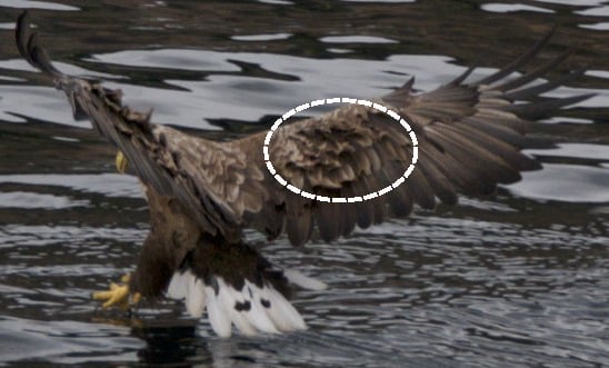
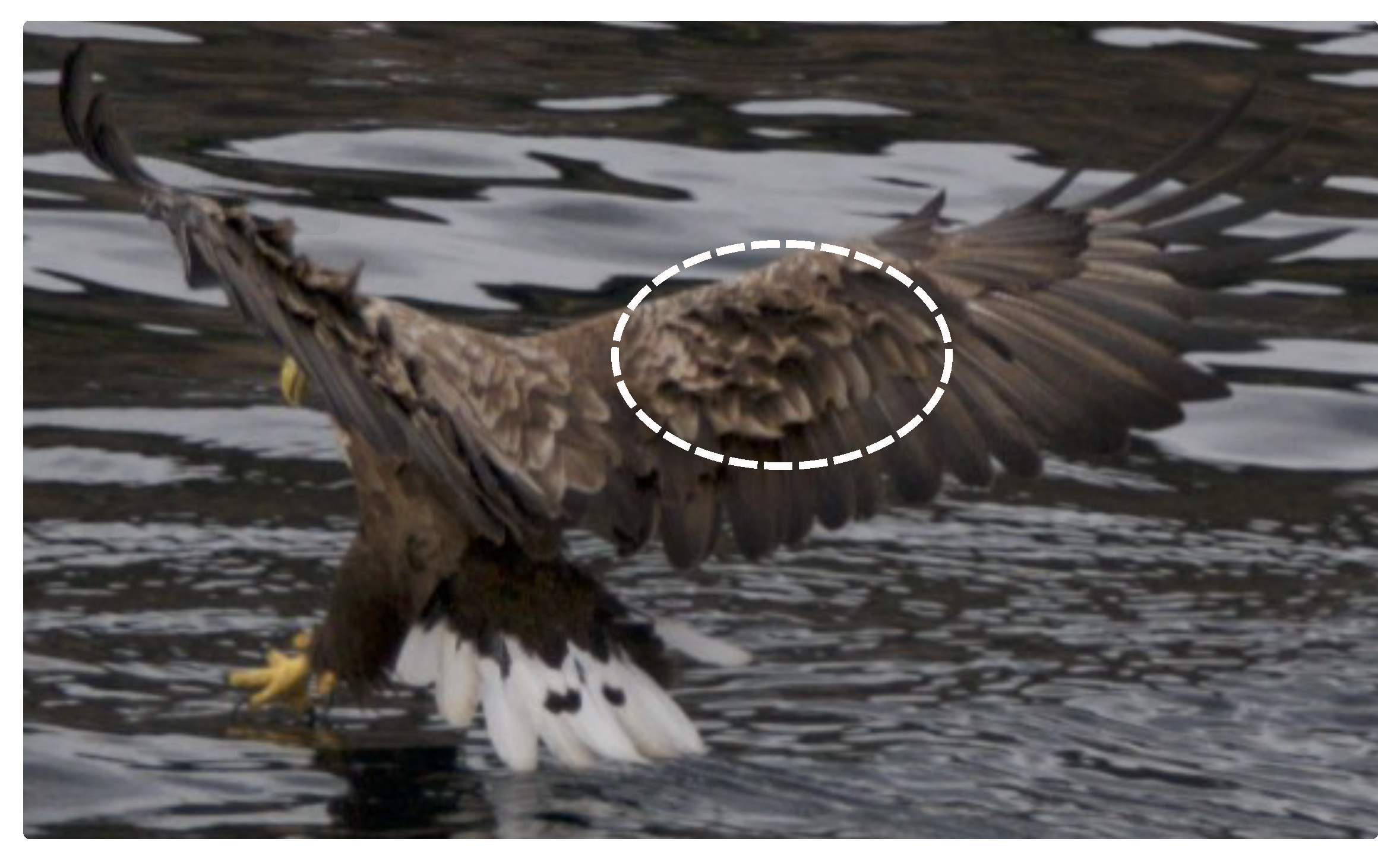
Passive feathers on the wings of birds provide one possibility to control flow separation in critical flight conditions, such as strong gusts or landing maneuvers [1]. Figure 1 shows the interaction of feathers for a white-tailed eagle trying to catch prey. In order to slow down, the bird increases the angle of attack of its wings. This could potentially lead to flow detachment starting from the trailing edge of the wing, which is known as stall. In this situation, self-adaptive feathers rise and prevent further detachment towards the leading edge of the wing. This interaction between feathers and flow allows for better control of lift at high angles of attack. This positive effect on the lift coefficient could be adopted for technical applications by replacing feathers with flexible flaps [2,3,4,5,6,7]. Examples for usage include small wind turbines, where strong gusts could lead to sudden drops in lift and therefore induce strong mechanical loads.

Table 1. Summary of the literature review with investigated profiles, Reynolds number Re of the flow, flap material, flexibility of the flap, and length with respect to the chord length of the profile c; ${}^1$ Experimental study; ${}^2$ Numerical study; ${}^3$ Polyethylene terephthalate.

Author	Profile	Re [$\times {10}^3$]	Flap Material	Flexible	Flap Length
Arivoli and Singh [3] ${}^1$	Plate	100	Cellulose acetate	yes	$0.08c-0.15c$
Brücker and Weidner [8] ${}^1$	NACA0020	77	Elastomer	yes	$0.05c-0.2c$
Favier et al. [7] ${}^2$	Cylinder	0.2	n/a	no	$0.2c$
Hafien et al. [10] ${}^2$	NACA0012	1.4–342	n/a	yes	$0.04c-0.11c$
Johnston et al. [6] ${}^{1,2}$	n/a	400	Polyester	no	$0.2c$
Kamps et al. [13] ${}^1$	Cylinder	13.5–34	Elastomer	yes	$0.3c$
Kernstine et al. [4] ${}^1$	NACA2412	330	Aluminum foil	yes	$0.1c-0.4c$
Liu et al. [9] ${}^1$	NACA0012	63	Mylar	yes	$0.25c$
Meyer [2] ${}^1$	HQ17/41	1000	Aluminum/PET ${}^3$	no	$0.084c-0.2c$
Rosti et al. [16] ${}^2$	NACA0020	20	n/a	yes	$0.1c-0.2c$
Schlüter [5] ${}^1$	NACA0012	30–40	Carbon fiber	no	$0.17c$
	NACA2213
	NACA4412
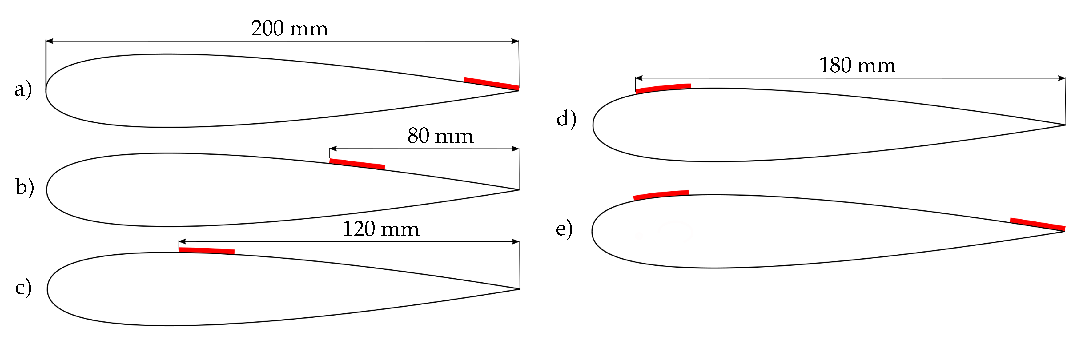
Talboys et al. [14,15] ${}^1$	NACA0012	50–350	Polyester	yes	$0.1c$

shows a summary of the previous publications on this topic. Based on this overview, the main influencing factors of flap performance are: (1) flap length, (2) flap shape, (3) flap position, (4) number of flap rows, and (5) flap material.

The effective flap length relative to the chord length c of the profile is in the range of $0.1c$ and $0.4c$. Brücker and Weidner [8] showed that a flap length of over $0.4c$ provided no positive effects. On the one hand, short flaps do not provide enough interaction with the flow to avoid stall. On the other hand, very long flaps cause a chaotic flutter and thus a decrease in lift. In a more detailed investigation about chaotic motion, Meyer [2] reported that the lift increase depends on the maximum angle between the flap and the profile surface. A positive effect on the lift coefficient was observed with an angle of up to 60${}^{°}$. Larger values caused a chaotic motion of the flaps, which terminated the positive effect on the lift. In order to prevent flutter motion or fall-over of the flaps, their length, thickness, and material properties, such as bending stiffness, are crucial.

Kernstine et al. [4] and Johnston et al. [6] reported additional drag on airfoils caused by flaps. This is in contrast to Liu et al. [9], who reported significant reduction in drag. In order to reduce the negative side effects of drag increase, Meyer [2] suggested changes in the flap shape. In an experiment with V-shaped flaps, he achieved a lift coefficient increase, while the drag coefficient was smaller compared to those of other flap shapes.

Arrivoli and Singh [3], Meyer [2], and Kernstine et al. [4] investigated the influence of the flap row position on a profile. Since these studies used different profiles (flat plate, sailplane profile, and NACA profile), the optimum flap positions were also different. Therefore, a general superior flap position can not be derived. Furthermore, the applied flaps were rigid or flexible, which suggests individual consideration of each study. The number of rows and its impact on lift coefficient was discussed by Meyer [2] and Hafien et al. [10]. Three rows increased the lift coefficient by up to 21% compared to a flapless profile. It seems that increasing the number of rows can prevent the flow separation more effectively. Another important factor for the placement of the flaps is the prediction of the flow separation point. Gault [11] and Bak [12] reported that the ratio of airfoil thickness to chord length has an impact on whether the separation starts from the trailing or leading edge. The study of Gault [11] delivered information for a broad range of NACA profiles and inflow Reynolds numbers from $6\times {10}^5$ to $2\times {10}^7$. Bak [12], on the other hand, offers a basic understanding for different stall characteristics. While the trailing-edge stall usually appears on thick profiles, the leading-edge stall is caused by a bursting laminar bubble at the leading edge.

Table 1 summarizes the flap materials used in recent research. They all have a low flap weight in common. Meyer [2], Schlüter [5], and Johnston and Edwards [6] used rigid flaps made of aluminum, PET, carbon fiber, or polyester. In the cases of flexible flaps, recent publications used aluminum foil [4], silicone elastomer [8,13], and cellulose acetate [3]. Flexible flaps produce less drag than rigid ones due to their better adaption to curved surfaces, such as NACA profiles [3,8]. Furthermore, they could lead to noise reduction. Kamps et al. [13] and Talboys et al. [14,15] investigated elastic flaps on the downstream side of a cylinder and airfoil in cross flow. Compared to profiles without flaps, they were able to reduce noise. This effect may have potential on small wind turbines in order to reduce sound emissions. In addition to the noise reduction, Talboys and Brücker [14] reported, in their study, on the shear layer stabilization effect that is caused by the trailing flaps on the suction side of the airfoil. This effect could also lead to enhanced airfoil performance.

This literature overview shows the benefits of flaps for a wide range of Reynolds numbers and the potential for technical applications. While the positive effect of the self-adapting mechanism is mentioned in the literature [3,4,8,9,16], there is only one study (by Kernstine et al. [4]) of elastic flaps with regard to lift and drag improvements. Because this study focuses on aluminum foil, there is a demand to investigate other elastic materials, since aluminum foil has the disadvantage of plastic deformation, which can be caused by strong gusts. This permanent deformation would negatively affect the aerodynamics of the airfoil. Hence, the main focus of this study will be the investigation of silicone flaps. Furthermore, experiments will be performed with a constant Reynolds number, as well as with varying inflow velocity, to investigate the influence of gusts. Drag and lift coefficients will be measured to conclude the benefits of flexible flaps.

2. Experimental Setup of the Force Measurements

2.1. Settings and Measurement Preparations

The experiments in this study were performed in a Göttingen-type wind tunnel (see Figure 2a) at the Chair of Fluid Dynamics and Turbomachinery at the TU Bergakademie Freiberg. The NACA0020 profile with a chord length c of 200 $\mathrm{m}$$\mathrm{m}$ was mounted on a force balance, as shown in Figure 2a,b. The force balance was placed downstream from the wind tunnel nozzle, which created a top-hat velocity profile suitable for the measurements. The height h and width w of the nozzle were 500 $\mathrm{m}$$\mathrm{m}$ and 600 $\mathrm{m}$$\mathrm{m}$. The maximum velocity of the wind tunnel in the open jet configuration was 40 m/s.

Figure 2b shows a more detailed picture of the airfoil mounted on the force balance. For a better overview of the components, the sketch illustrates a cross-sectional cut in the middle of the profile, and thus shows only one half of the profile. The NACA0020 profile was used, since it is a simple baseline profile and has been studied thoroughly. Furthermore, it is quite common for small wind turbines. End plates were placed on each side of the profile to suppress tip vortices and improve the two-dimensionality of the flow. Moreover, the angle of attack $\alpha$ of the profile can be changed with respect to the direction of flow. By measuring lift $F_L$ and drag forces $F_D$, it is possible to generate polar diagrams to characterize the performance of the profile near the stall. The forces were recorded and averaged over a time period of 10 $\mathrm{s}$ with a sampling rate of 50 $\mathrm{Hz}$. Finally, the lift $c_L$ and drag coefficients $c_D$ were calculated as follows:

$$\begin{array}{cc}\hfill c_L& =\frac{2·F_L}{\rho ·U_0^2·A},\hfill \end{array}$$

(1)

$$\begin{array}{cc}\hfill c_D& =\frac{2·F_D}{\rho ·U_0^2·A}.\hfill \end{array}$$

(2)

where $\rho$ denotes the density of air, and $U_0$ the inflow velocity. The chord area A (see Figure 2b) is a product of c and the total profile width, which is 600 $\mathrm{m}$$\mathrm{m}$.

In the first part of this investigation, lift and drag coefficients were measured for different flap configurations. The measurements were performed at a constant flow velocity of $U_0$ = 15 m/s. This resulted in a Reynolds number of approximately $2\times {10}^5$. During the measurements, the angle of attack of the profile was varied from ${\alpha }_{\mathrm{Start}}=0{}^{°}$ to ${\alpha }_{\mathrm{End}}=25{}^{°}$ in order to analyze the pre-stall and stall region performance. Lift and drag forces for a flapless profile were also measured for reference.

In the second part of the force balance measurements, the lift and drag forces of the NACA profile were analyzed with and without flaps in a transient flow. Periodical gusts were generated by a rotating plate, as shown in Figure 2a. This plate altered the flow resistance of the air flow in the wind tunnel. This resulted in a sinusoidal velocity magnitude in the open jet section with a frequency of $0.5$ $\mathrm{Hz}$ and a peak-to-peak amplitude of 1 m/s. Due to the additional flow resistance, the average flow velocity was reduced to 14 m/s. The number of flap rows and their positions were taken from the first part of the investigations.

2.2. Preparation of Flaps

The flaps were produced by cutting into a large sheet of elastomer foil with a total width and length of 600 and 30 $\mathrm{m}$$\mathrm{m}$, respectively. Since the length of the flaps themselves was only 20 $\mathrm{m}$$\mathrm{m}$, they were connected to each other at the top of the sheet (see Figure 3). Therefore, if one flap starts moving, it likely induces movement of its neighbors. The top 10 $\mathrm{m}$$\mathrm{m}$ of the elastomer sheet was used to attach the flaps with adhesive tape to the airfoil (green shaded area in Figure 3). In order to stop cracks from forming at the ends of the incisions between the individual flaps, each cut was terminated with a particular hole to prevent stress concentration.

Five different combinations of flap positions were investigated, as shown in Figure 4. First, the position of a single flap row on the NACA0020 profile was analyzed. Afterwards, a combination of flaps at the leading and trailing edges was investigated. It is assumed that a combination of both configurations provides better stabilization of the flow at the critical angle. While the trailing-edge flap suppresses flow instabilities at the trailing edge of the profile, it is assumed that the leading-edge flaps may impact two mechanisms. Firstly, the leading-edge flaps can counteract the turbulent separation that is formed at the trailing edge at smaller angles and that moves with an increasing angle of attack towards the leading edge (as observed by Balduzzi et al. [17] for a similar profile). Secondly, the leading-edge flap could influence vortices that are formed at the leading edge after the flow separation (as observed by Hsiao et al. [18] and Liu et al. [9]).

The flaps were made of silicone (Figure 5, left) and provided by FILK (FILK—Forschungsinstitut für Leder und Kunststoffbahnen in Freiberg, Germany).

Table 2. Material properties of the flaps.

Thickness	$200.0$ $\mathsf{\mu }$$\mathrm{m}$
Density	1155.0 kg/m${}^3$
Ultimate tensile strength	13.8 N/mm${}^2$
Tear propagation resistance	2.0 N
Bending stiffness	10.9$·$10${}^{-2}$ N$·$mm${}^2$

presents the material properties for the silicone foil. The foil has a total thickness of 200 $\mathsf{\mu }$$\mathrm{m}$ and a low bending stiffness; thus, it adapts well to the curved surface of the NACA0020 profile, as shown in Figure 5 (right). Furthermore, this material has sufficient tensile strength and tear propagation resistance to withstand shear forces.

3. Results and Discussion

3.1. Literature Validation and Uncertainty of Measurement

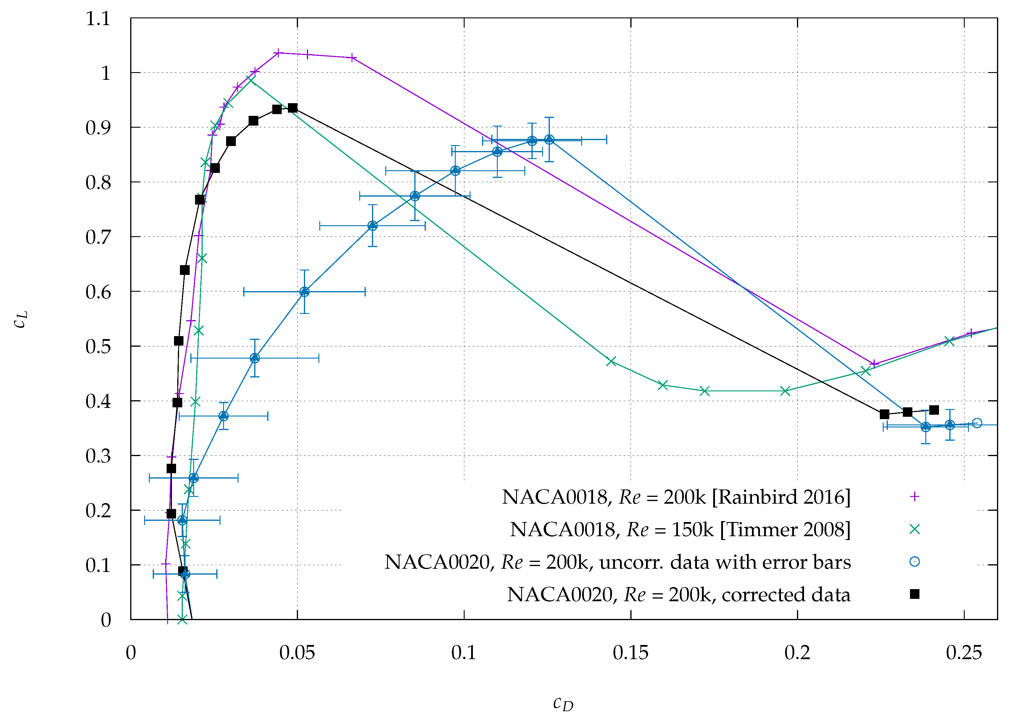
In the following section, results from the flapless profile of the present study and from other publications are compared in order to validate the measuring system. Unfortunately, no other data sets of polars were found for same profile and Reynolds number. Therefore, results of an NACA0018 are included with similar $Re$ values by Timmer [19] and Rainbird [20] (see Figure 6). For this comparison, a correction method is employed that was proposed by Du et al. [21] for open-jet wind tunnels. This method is based on Garner et al. [22], and considers the effect of streamline curvature. The cause for this effect is the diverging jet, which expands even more with an increasing angle of attack of the airfoil. The correction equations are as follows:

$$\begin{array}{cc}\hfill c_{L,corr}& =c_L+c_L\frac{{\pi }^2}{24}{\left(\frac{c}{\beta h}\right)}^2,\hfill \end{array}$$

(3)

$$\begin{array}{c}\hfill \beta =\sqrt{|1-M{a}^2|}\approx 1.\end{array}$$

(4)

Hereby, $c_{L,corr}$ is a function of the uncorrected lift coefficient $c_L$, chord length c, and wind tunnel nozzle height h. $\beta$ is a function of the Mach number $Ma$ and has a value of approximately 1 because of the low inflow velocity during the experiments. The corrected drag coefficient $c_{D,corr}$ considers the geometry of the nozzle and is calculated as follows:

$$\begin{array}{cc}\hfill c_{D,corr}& =c_D-\frac{1}{2\pi }\left(\frac{L_0}{L}-1\right)c_L^2,\hfill \end{array}$$

(5)

$$\begin{array}{cc}\hfill \frac{L_0}{L}& =1+\frac{\pi c}{2h}.\hfill \end{array}$$

(6)

Figure 6 shows a good agreement between the literature and the experimental data. However, the lift coefficient in our study is underestimated by up to 10% compared to Rainbird [20]. The comparison of our study with Timmer et al. [19] shows the same trend, with a difference of up to 5%. Rainbird and Timmer both used a closed section of measurement, which is assumed to be the main reason for this difference. A similar observation between closed and opened sections of measurement was reported in the study of Du et al. [21]. Furthermore, it is assumed that the slight vibrations of the profile are the cause of standard deviation, which is presented by the error bars in Figure 6. The general purpose of standard deviation is to represent random error of the measurements. At the critical angle, the deviation for $c_L$ is ±5%; for $c_D$, it is ±8%. Despite the standard deviation, repeated experiments of three test series showed an error between mean values of less than 1%.

For our measurements, the airfoil was placed in the center of the wind tunnel nozzle. The flow is uniform and has a turbulence intensity of less than 0.1%. The major impact on accuracy of the calculated coefficients resulted from velocity, force, and density measurements. The load cells of the force balance have a deviation of ±0.04 N. The temperature and ambient pressure needed for density calculation have a deviation of ±$0.5$ ${}^{°}\mathrm{C}$ and ±100 $\mathrm{Pa}$, respectively. The velocity at the nozzle outlet is measured through the pressure difference between the nozzle and the environment, and has a deviation of ±0.073%. To guarantee a constant velocity, the number of revolutions per minute of the fan are kept constant (about 460 min${}^{-1}$). Finally, an overall calculation of the uncertainty propagation for multiple variables delivers a maximum deviation of ±1.0% for $c_L$ and ±4.2% for $c_D$. The estimated measurement uncertainty for the lift coefficient is rather constant, while the relative error of the drag coefficient is largest for angles smaller than 6${}^{°}$. This is due to the constant deviation of the load cells and the small measured forces at low angles. With increasing angle (6${}^{°}$), the estimated measurement uncertainty drops to less than 1.0%.

It should be noted that uncorrected data (drag, lift, and angle of attack) are presented in this publication; there are two reasons for this: (i) The correction method supposes two-dimensional flow. For flapped configurations at critical angles and in the stall region, this is not guaranteed. (ii) There is more than one correction method (e.g., [17,22]). Therefore, the uncorrected data can be used by other authors and adapted to their needs. Furthermore, the aim of our study is to present the trends of the lift and drag coefficients, which are still guaranteed by the uncorrected data.

3.2. Steady Flow Conditions

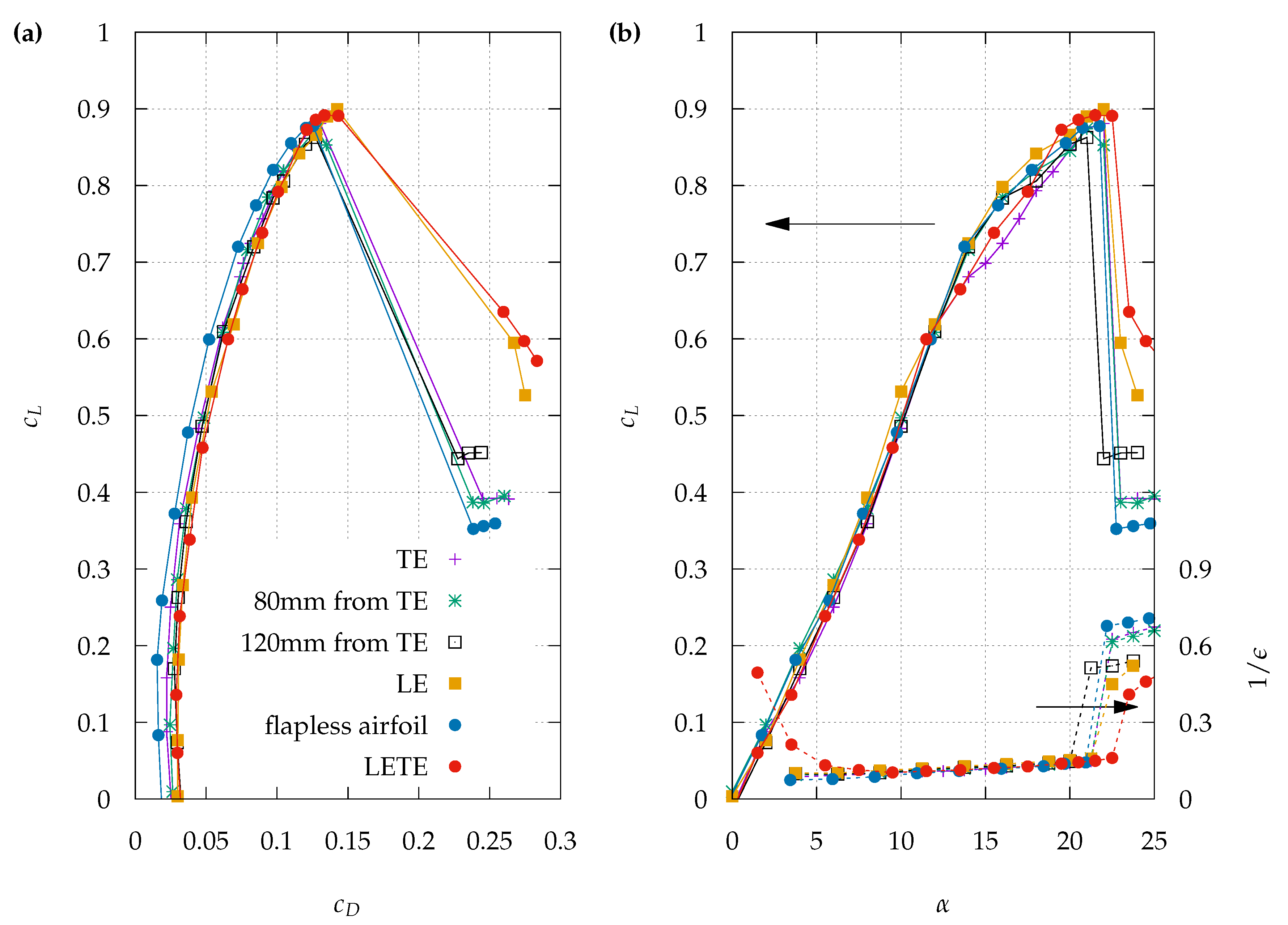
Figure 7a shows a lift–drag polar for one silicone flap row for four different positions on the NACA0020 profile and a combination of two rows at the leading and trailing edges. Figure 7b gives the reciprocal lift-to-drag ratio $ϵ$ and lift coefficient against the angle of attack. Hereby, the reciprocal lift-to-drag ratio is calculated with:

$$\begin{array}{cc}\hfill \frac{1}{ϵ}& =\frac{c_D}{c_L}.\hfill \end{array}$$

(7)

$ϵ$ is an essential parameter for qualification of rotor blades on a wind turbine because of its influence on the power output. Hence, reciprocal values were added for better presentation of the curve; they also allow a more detailed analysis with respect to the angle of attack. In both diagrams, data of a profile without flaps are included for reference.

For angles lower than 15${}^{°}$, the flapless profile generates up to 50% less drag than other flapped configurations. The slight increase in drag with flaps compared to the baseline airfoil can be explained by the surface unevenness caused by the flaps. The flap row configurations of trailing edge (TE), 80 $\mathrm{m}$$\mathrm{m}$ from TE, and 120 $\mathrm{m}$$\mathrm{m}$ from TE offer no benefits in the pre-stall region. The maximum lift coefficient in the pre-stall region increases only for two configurations: Flap row at the leading edge and flap row at the leading and trailing edges of the airfoil. For these two cases, a lift coefficient increase of up to 2.5% and drag coefficient increase of 12% are observed at the critical angle. The additional drag at the critical angle results from raised flaps that cause higher flow resistance. Nevertheless, considering the angle delay that is achieved by the leading-edge (LE) and leading-edge–trailing-edge (LETE) configurations, a comparison of these configurations at the critical angle with the same angle of the flapless profile shows an increase of up to 2.5 times for $c_L$ and a reduction by 40% for $c_D$.

Furthermore, the reciprocal value of $ϵ$ is constant for all configurations between angles 6${}^{°}$ and 20${}^{°}$. Because 1/$ϵ$ becomes very large at small angles, no values were considered for angles less than 3${}^{°}$, except for the LETE configuration for the purpose of example presentation. The divergence of 1/$ϵ$ results from very small lift coefficients at low angles of attack. The LETE configuration has an $ϵ$ minimum at 4${}^{°}$, which is a consequence of the flaps. Because of the two flap rows on the upper airfoil surface, the drag coefficient is slightly higher, while the lift coefficient value remains rather small.

Compared with the flapless airfoil, the flow separation was delayed by approximately $0.5$${}^{°}$ for the LE configuration and by 1${}^{°}$ for the LETE configuration. During the experiment, the flaps started to move permanently at the critical angle. At lower angles of attack, there was almost no interaction with the flow. At the critical angle of attack, it seems that the slightly raised flaps influence the backflow region, which was also observed by Brücker and Weidner [8]. Despite that, it should be noted that the raising of the flaps in a wind tunnel at the critical angle is less distinctive in comparison with the water channel results in [8], which is likely a consequence of the density ratio difference between the fluids and flaps.

The positive effects of the flapped configurations can especially be seen in the stall region. Depending on the flap row position, the lift coefficient after flow separation increases by up to 50% (for the LE and LETE configurations). This lift increase is in good agreement with the results of Hsiao et al. [18], who reported a lift enhancement of between 50% and 70% for the stall region. Moreover, the increasing lift of the LETE configuration in the stall region affects 1/$ϵ$, as it has the lowest values from all configurations. For the configurations TE, 80 $\mathrm{m}$$\mathrm{m}$ from TE, and 120 $\mathrm{m}$$\mathrm{m}$ from TE, the lift coefficient increase during the stall is between 10% and 20%, respectively. From the $c_L$ evaluation of the LE, LETE, and 120 $\mathrm{m}$$\mathrm{m}$ from TE configurations, it seems that the closer the flaps are placed to the leading edge, the better the airfoil performance in the stall region is.

3.3. Smoke–Wire Flow Visualization

3.3.1. Experimental Setup

Because the force balance results allow a limited explanation regarding the acquired results, a visualization of the flow was done. This technique provides a better possibility of comparison and evaluation of the flow around the airfoil with and without flaps.

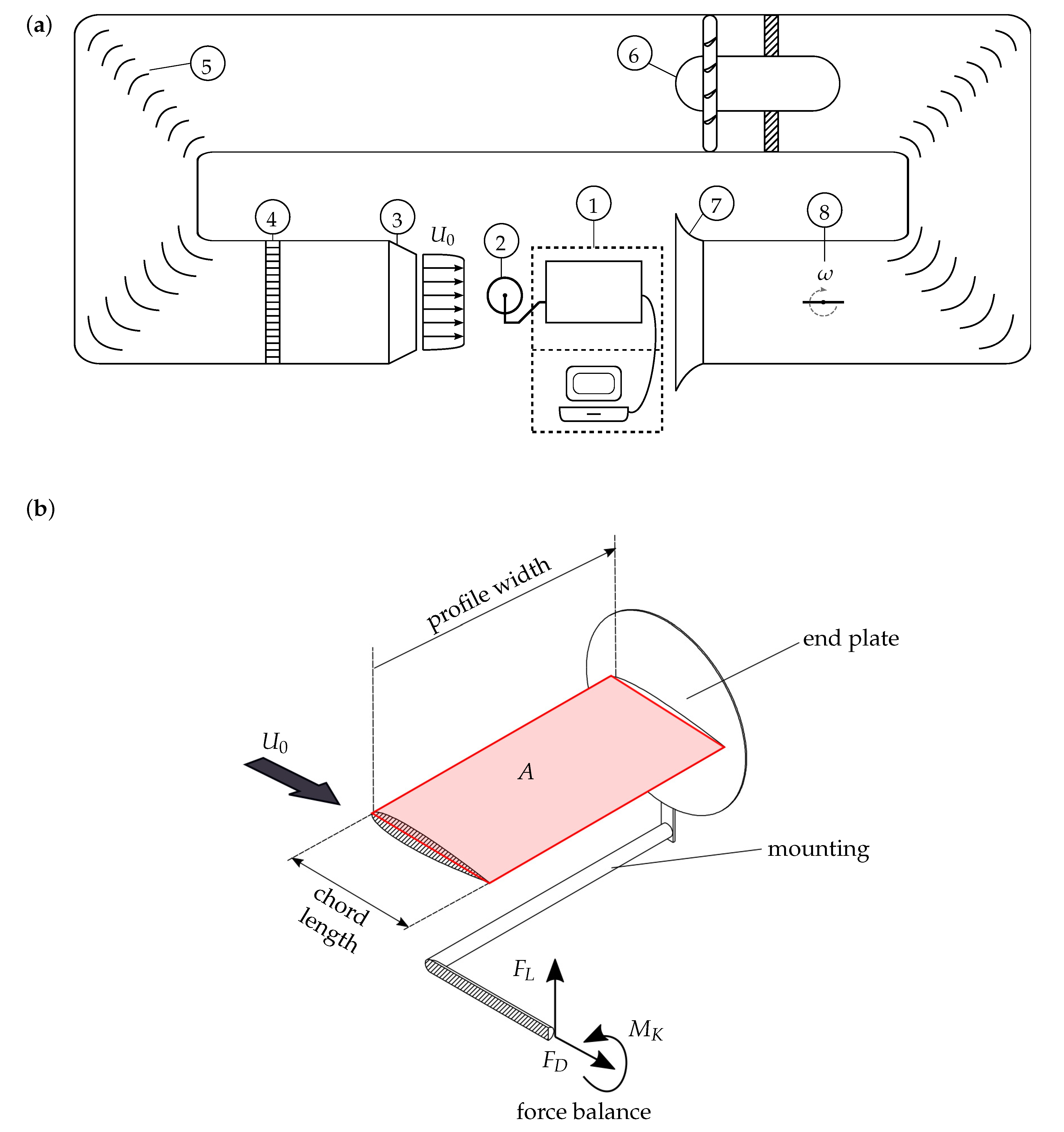
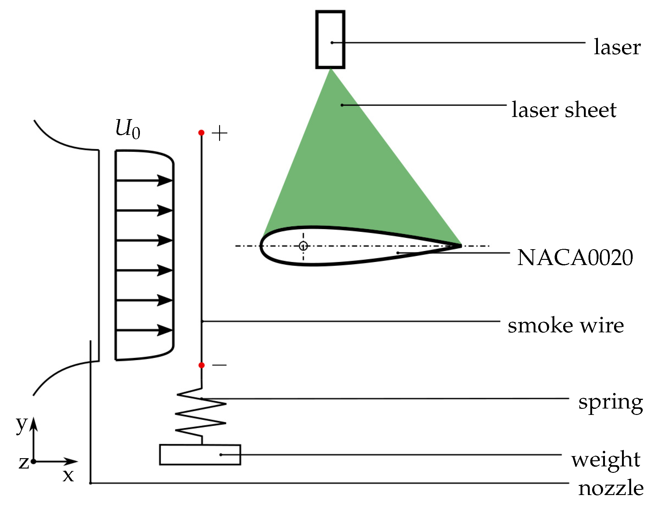
The experimental setup is illustrated in Figure 8. This smoke–wire technique is adapted from Kirk et al. [23]. The NACA0020 profile was mounted in the test section without end plates in order to see the flow around the airfoil surface. A vertical Nichrome wire with a thickness of $0.1$ $\mathrm{m}$$\mathrm{m}$ was placed $0.1$ $\mathrm{m}$ in front of the profile. During the inflow, the wire was stabilized by a spring and weight that damped the vibrations caused by the flow. Furthermore, the wire was connected to a power supply unit that provided 30 $\mathrm{V}$ and 5 $\mathrm{A}$ direct current. On the wire, a manual application of a mixture (Glycerin 70% and water 30%) was done with a cotton swab. The inflow velocity of 15 $\mathrm{m}$ ${\mathrm{s}}^{-1}$ was adjusted. In order to visualize smoke, the vertical wire was placed on the same plane as the laser sheet, which was in the middle of the airfoil. The laser sheet was generated by a 10 mJ Nd:YLF high speed laser.

The pictures of the illuminated smoke flow were taken by a high-speed camera (Phantom V12.1) that was placed perpendicularly to the laser sheet. The frame rate was 2000 $\mathrm{Hz}$ and exposure time 70 $\mathsf{\mu }$$\mathrm{m}$, with a resolution of 1280 × 800 (35.5 pixels per 1 $\mathrm{c}$$\mathrm{m}$). The images were averaged in order to visualize the flow field and the recirculation region. Only steady flow conditions can be investigated with this setup due to the short smoke generation time of less than $0.5$ $\mathrm{s}$.

3.3.2. Flow Visualization Results

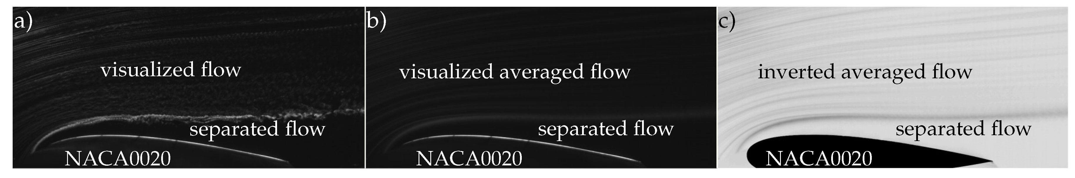
Figure 9 shows the post-processing procedure, as well as the possibilities and limits of this visualization technique. For example, a flapless airfoil was selected with $\alpha$ = 20${}^{°}$. Considering the literature [17,23], at this angle, turbulent separation is formed and proceeds to move from the trailing edge towards leading edge, which makes it a convenient example.

Figure 9a shows a snapshot of the visualized flow around the NACA0020 profile. Since the size of the turbulent separation region is time-dependent, it is necessary to generate an averaged flow field (see Figure 9b) in order to evaluate the results. The averaged flow field for this configuration consists of five different measurement series, with each containing up to 200 snapshots. With this approach, it was possible to confirm the repeatability of the observed results. At last, the averaged flow field was inverted and the contrast was increased to improve the visualization (see Figure 9c). Additionally, a mask of the NACA0020 profile was added for a better differentiation between the fluid flow and the airfoil.

With this setup, it is not possible to visualize the boundary layer at the airfoil surface. As seen in Figure 9c, the turbulent separation is not directly visible. The reason is the smoke, which flows only around separation regions. Moreover, the vortices that guide the smoke into the turbulent separation favor the mixing process of smoke and air, which additionally limits the visualization of the separation regions (see Figure 9c). Nevertheless, despite not seeing the mechanism inside the separation region, it is still possible to visualize the laminar flow around the airfoil. Thus, the size and location, especially for the turbulent separation region, can be visualized indirectly, as the contours around it are visible. However, the discussion in this chapter focuses on flap interaction in the deep stall region. With the current setup, the boundary layer cannot be visualized, and no clear differences were observed for the airfoil with and without flaps in the pre-stall region.

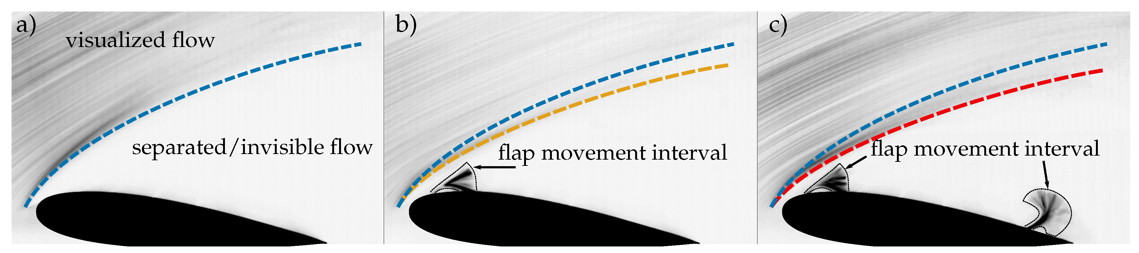
Figure 10 shows the flow field for a flapless profile and the flapped configurations LE and LETE at $\alpha$ = 25${}^{°}$. The turbulent recirculation region is formed above the airfoil. For a flapless airfoil, the recirculation region appears to be larger than in the cases of the LE and LETE configurations. The flap movement interval (see Figure 10b,c) indicates a backflow from the trailing edge towards the leading edge. However, unlike the leading-edge flap, the trailing-edge flap is permanently turning over (see Figure 10c). Because of the force balance measurements, the increased performance of this configuration is known during deep stall, and it seems that the turn-over movement is crucial for the airfoil performance. Unfortunately, it was not possible to visualize the flow in the separated region. It is assumed that the turned-over flaps at the trailing edge influence the intensity and velocity of the separated flow at the upper surface of the airfoil.

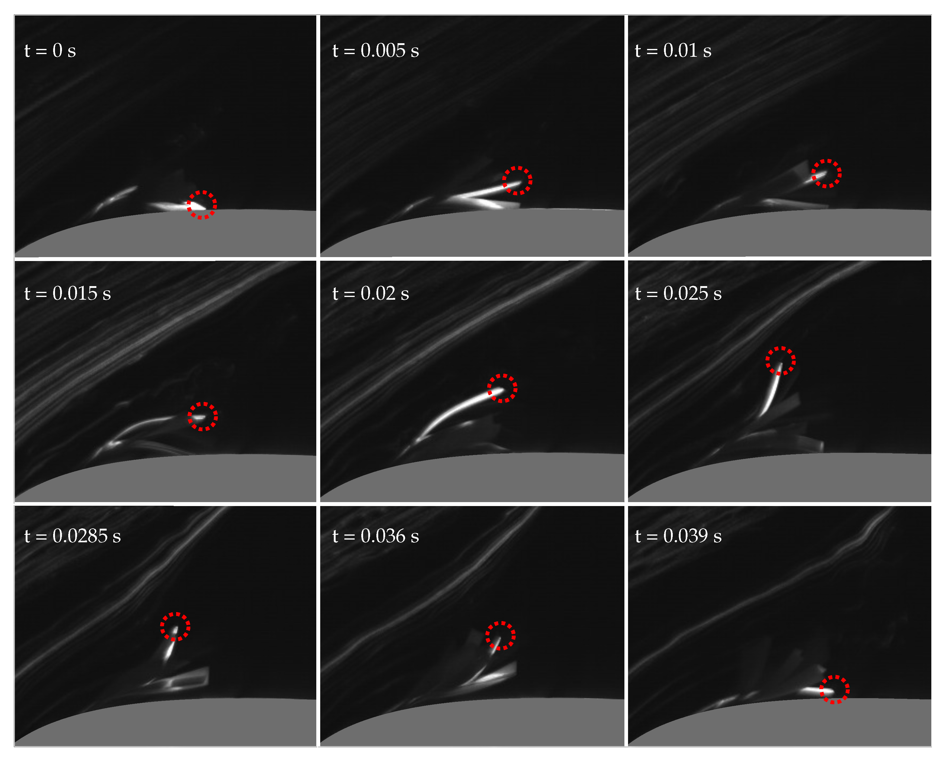
Figure 11 presents snapshots of the flap motion for one cycle. The cycle includes an upward motion of the flap from the airfoil surface and a pull-back motion. The backflow inside the turbulent separation region raises the elastic flaps from the airfoil surface so they reach into the laminar flow. At this point, elastic flaps are pushed back by the aerodynamic forces of the ambient flow. The push-back motion appears to be similar to a whip movement, as it was repeatedly observed to be up to three times faster than the upward motion. It is supposed that this movement pushes the vortices down towards the airfoil surface. As a consequence, the instantaneous laminar flow leans more towards the airfoil and the recirculation region shrinks, which was observed previously in Figure 10. Due to the conservation of momentum, the pushed-down vortices generate lift.

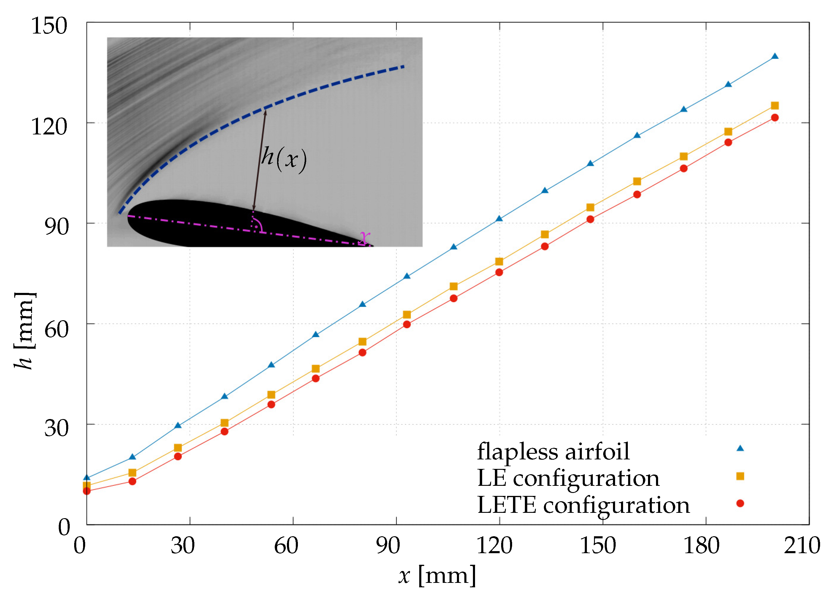
Figure 12 summarizes the results of the turbulent separation regions around the NACA0020 profile for the flapless airfoil, LE, and LETE configurations at $\alpha$ = 25${}^{°}$. This figure allows a more precise evaluation of the distance h between the separation line and the airfoil surface at position x of the chord line. The evaluation is performed manually with a graphic editor due to the need for individual contrast adaption of each configuration. Nevertheless, the deviation of this method is about 1 px, which provides a proficient accuracy. The distance between the separation line and the airfoil surface increases with growing x for the flapped and flapless configurations. For the LE and LETE configurations, the separation lines show smaller distance differences compared to those of the flapless profile. The height difference of the flapped configurations is constant and does not increase towards the trailing edge of the profile. With the current method, it was not possible to visualize and evaluate the vortices in the turbulent separation region, as they seem to influence the lift coefficient in deep stall. Thus, the recirculation size evaluation delivers no explanation for the lift coefficient difference between the LE and LETE configurations in deep stall.

3.4. Gust Simulation

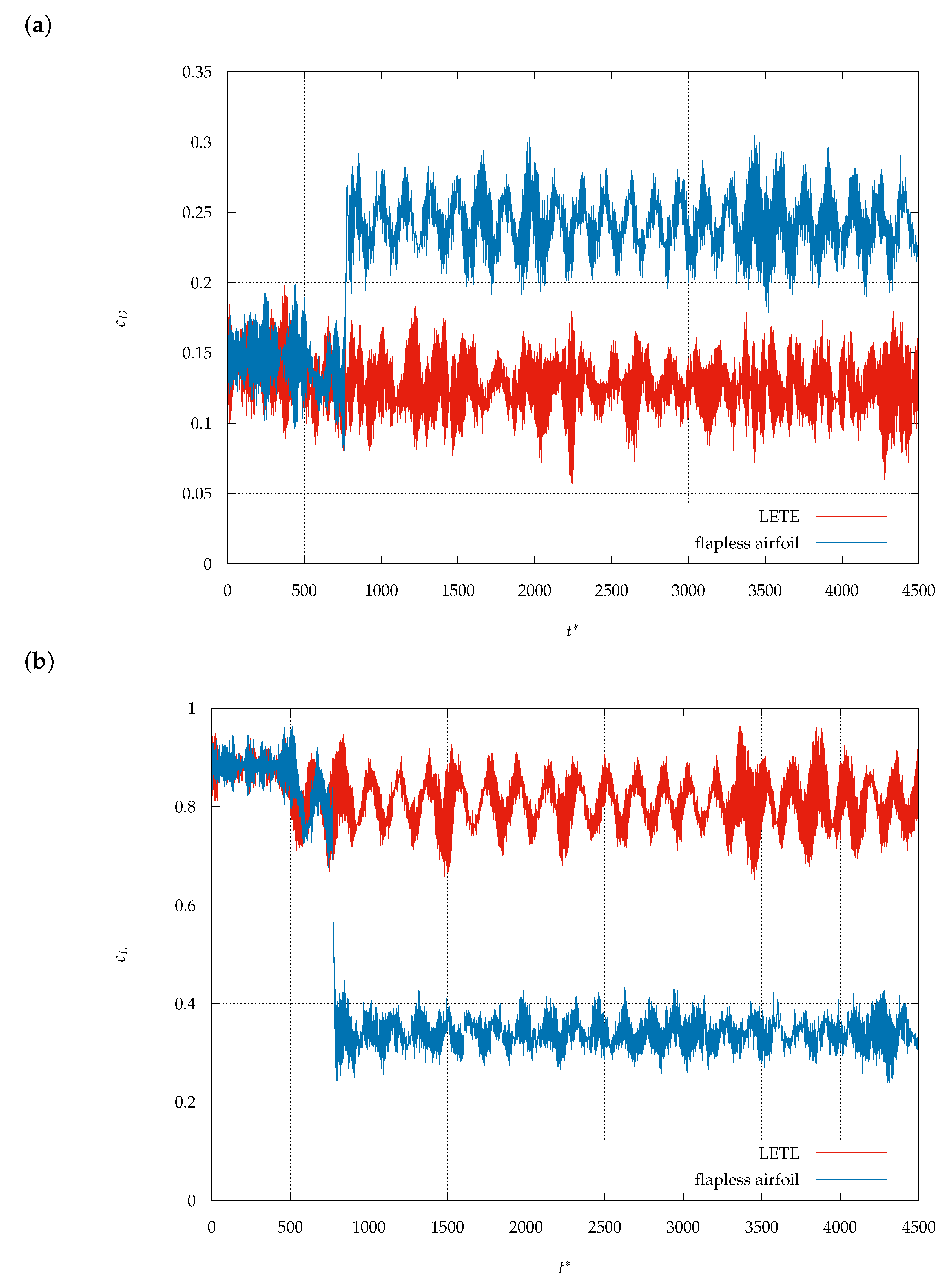
Figure 13 shows results of drag and lift coefficients in a gust simulation for the NACA0020 profile with and without flaps. The flapped profile has flaps at the leading and trailing edges, as this was the best configuration under steady flow conditions. The angle of attack is set slightly below the critical angle. For the flapped configuration, the angle is approximately $22.5$${}^{°}$, and for the flapless profile, it is about $21.5$${}^{°}$. The coefficients $c_L$ and $c_D$ in Figure 13 depend on dimensionless time $t^{*}$:

$$\begin{array}{cc}\hfill t^{*}& =\frac{t·U_0}{c}.\hfill \end{array}$$

(8)

The coefficients were measured for a time interval of t = 60 $\mathrm{s}$. Until $t^{*}$≈ 750, the flow is steady with an adjusted velocity $U_0$ = 15 m/s. After $t^{*}$≈ 750, gusts are initiated by the rotating plate and the flow becomes transient. The average flow velocity reduces to 14 m/s. This is due to the increase in flow resistance of the rotating plate in the wind tunnel. The resulting sinusoidal velocity profile has a frequency of $0.5$ $\mathrm{Hz}$ and a peak-to-peak amplitude of 1 m/s. The lower flow velocity, and thus the lower Reynolds number, leads to a reduction in the critical angle of attack [5]. This effect triggers flow separation.

The drag coefficients for a profile with and without flaps are presented in Figure 13a. The drag coefficient of the profile without flaps increases suddenly after gust initiation. This indicates that stall is occurring, which raises the drag coefficient by 38%. In contrast, the average drag coefficient for the profile with flaps decreases slightly by only 13%. As mentioned above, this reduction is due to the lower flow velocity resulting from the rotating blade in the wind tunnel. Lift coefficients for the NACA profile with and without flaps are shown in Figure 13b. While gusts reduce the lift coefficient of the flapless profile by more than 60%, the flapped profile is only marginally influenced, with a reduction of about –5%. It should also be noted that during the gust initiation, drag coefficient fluctuations are similar for the flapped and flapless profiles, while the lift coefficient fluctuations increase. For the flapped profile, these lift coefficient fluctuations are two times higher than those of the flapless profile. This significant difference probably results from increasing dynamic loads on the profile at the critical angle and thus stronger back-and-forth movements of the airfoil and mounting.

For the flapless profile, the flow separation set in shortly after the lowest velocity was reached (see Figure 13a). This outcome was observed repeatedly during gust simulations. Since stall tends to set in earlier with decreasing Reynolds numbers, this velocity reduction destabilizes the flow and causes the onset of flow separation on the flapless airfoil. Flap rows at the trailing and leading edges reduce the impact of the gusts through interaction with the flow. The main result of this is the prevention of precociously appearing flow separation.

4. Conclusions

The aim of this study was to investigate the drag and lift for an NACA0020 profile with and without elastic flaps. Experimentally, the drag and lift forces were measured using a force balance in a Göttingen-type wind tunnel. Five different flap configurations were investigated in steady states and one configuration in transient flow.

In the first part, flaps were investigated using steady flow conditions. Using a single flap row on the profile, a significant increase in lift was observed in the post-stall region, and stall was delayed by $0.5$${}^{°}$. The leading-edge flap configuration achieved the best performance. Furthermore, in the pre-stall region, the drag coefficient is noticeably higher in comparison to that of the flapless profile. This increase resulted from additional friction losses due to the flaps on the profile surface. Since the flow separation develops from the trailing edge, another flap row was added at the end of the NACA0020 profile. The two-flap row combination offered the most beneficial impact on the results with respect to post-stall lift increase and stall angle delay.

In the second part, a smoke–wire visualization technique was used for a better understanding of the airfoil performance improvement by the flaps in the deep stall region. Hereby, a comparison of flapless airfoil, flaps at the leading edge, and flaps at the leading and trailing edges was done. It was shown that the leading-edge flaps push the averaged flow field towards the airfoil surface. This causes a reduction of the turbulent recirculation region size and improves the performance of the airfoil.

Finally, experiments were performed for the NACA0020 profile with and without flaps under transient flow conditions. Flaps were placed at the leading and trailing edges. The angle of attack was set to its critical value. Once the gusts started, the drag coefficient of the flapless profile increased by nearly 60%, while the lift coefficient fell significantly. The combination of gusts and the critical angle lead to stall. In contrast, the flapped profile offered a significantly better performance. After initiating the gusts, drag and lift decreased only by about 6% and 5%, respectively. This indicates that stall is prevented by the NACA profile with flaps. As soon as the stall starts to develop at the leading edge of the profile, the flaps rise from the surface and prevent further spreading of the flow separation.

For a better understanding of the interaction between flaps and flow under stall conditions, future work will focus on PIV measurements of the near-wall flow. Furthermore, fiber-reinforced flap materials suitable for higher loads will be investigated because they could be potentially used with small wind turbines.