Hydrodynamic Equilibrium Simulation and Shut-in Time Optimization for Hydraulically Fractured Shale Gas Wells

Abstract

Post-fracturing well shut-in is traditionally due to the elastic closure of hydraulic fractures and proppant compaction. However, for shale gas wells, the extension of shut-in time may improve the post-fracturing gas production due to formation energy supplements by fracturing-fluid imbibition. This paper presents a methodology using numerical simulation to simulate the hydrodynamic equilibrium phenomenon of a hydraulically fractured shale gas reservoir, including matrix imbibition and fracture network crossflow, and further optimize the post-fracturing shut-in time. A mathematical model, which can describe the fracturing-fluid hydrodynamic transport during the shut-in process, and consider the distinguishing imbibition characteristics of a hydraulically fractured shale reservoir, i.e., hydraulic pressure, capillarity and chemical osmosis, is developed. The key concept, i.e., hydrodynamic equilibrium time, for optimizing the post-fracturing shut-in schedule, is proposed. The fracturing-fluid crossflow and imbibition profiles are simulated, which indicate the water discharging and sucking equilibrium process in the coupled fracture–matrix system. Based on the simulation, the hydrodynamic equilibrium time is calculated. The influences of hydraulic pressure difference, capillarity and chemical osmosis on imbibition volume, and hydrodynamic equilibrium time are also investigated. Finally, the optimal shut-in time is determined if the gas production rate is pursued and the fracturing-fluid loss is allowable. The proposed simulation method for determining the optimal shut-in time is meaningful to the post-fracturing shut-in schedule.

1. Introduction

Shale gas reservoir development mostly uses multi-stage fracturing technology in large-scale horizontal wells, but field data indicate that only 15%–30% of the fracturing water is recovered after the flowback [1], which is very low compared with conventional reservoirs. Although the initial production of shale gas fractured wells is relatively high, the production decreases rapidly and the stable production period is usually short [2]. In order to improve productivity after fracturing, energy-storage fracturing is adopted in the field. This fracturing management mode is characterized by long-term shut-in to diffuse bottom-hole pressure to the formation instead of immediately flowing back after fracturing. However, there is also a view in academia that the shut-in process will cause further imbibition of fracturing fluid from hydraulic fractures to form water-phase traps, resulting in reservoir damage [3]. Therefore, it is a controversial issue whether shut-in after fracturing is beneficial to production.

The traditional approach to well shut-in after fracturing is to close the fracture elastically, so as to compact the proppant and prevent proppant reflux in the process of flowback. The shutdown time is very short. The simulation of shut-in after fracturing focuses on the variation of the pressure field and the water saturation field in a reservoir during shut-in. Physical experiments and numerical simulations have been carried out by different scholars from core to field scale. Dutta et al. [4] used real-time CT scanning to observe the distribution of fracturing fluid in a core. The results show that the water phase saturation redistributes in the core during the shut-in period. It specifically appears that the water phase saturation at the injection end decreases, and the water phase saturation increases at the distal core. Seven days after shut-in, the water saturation front reached 67% of the sample length, which indicates that, during shut-in, the fracturing fluid will enter the reservoir matrix by imbibition and then increase the water saturation of the matrix. At the same time, it can be seen that the water saturation curve after simulated backflow basically coincides with that at 7 days after shut-in, which indicates that it is difficult for the water in the matrix to flow after 7 days of shut-in, and further explains the phenomenon of a low backflow rate of fracturing fluid in tight reservoirs. Wang and Leung [5] used the commercial simulator Computer Modeling Group (CMG) to simulate the backflow and retention of fracturing fluid after large-scale hydraulic fracturing. Their simulation study shows that, during shut-in, the water in the fracture will permeate into the matrix, and with the increase of shut-in time, the infiltration range will increase, which will promote oil entering the fracture and increase the initial production. However, prolonging the shut-in time will only increase the initial production of the oil well, but it cannot sustain high production. Ghanbari and Dehghanpour [6] established a numerical model for Horn River Basin shale gas from fracturing fluid injection to backflow. The model was initialized by using the method of water injection to increase the pressure in the fracture and water phase saturation to simulate the initial state after fracturing. The research shows that prolonging the shut-in time after fracturing can increase the initial gas production obviously and reduce the fracturing fluid flowback rate, and capillary force has an important influence on flowback. An increase in capillary force can promote the occurrence of water flowing through porous media and cause a water lock in the matrix, but also reduce the initial gas production; complex fractures can help to increase gas production but reduce flowback rate; and with the increase of shut-in time, gravity differentiation is significant. Wang et al. [7] established a numerical model to investigate the chemical osmosis phenomena on fracturing-fluid leakoff during shut-in periods. Their simulation results indicate that chemical osmosis can lead to an extra leakoff volume of 7‰.

In this study, we link the hydrodynamic equilibrium phenomenon of a hydraulically fractured reservoir with the well shut-in schedule. A mathematical model is developed for numerical simulation of the fracturing-fluid crossflow and imbibition behaviors under different driving forces during the well shut-in process. The simulation results are used to establish a relationship between the reservoir hydrodynamic equilibrium and well shut-in time, and, further, to determine the optimal shut-in time for a hydraulically fractured shale gas well.

2. Hydrodynamic Equilibrium Mechanism during Well Shut-In

A hydraulically fractured shale gas reservoir experiences a complicated hydrodynamic equilibrium process during the well shut-in, which involves fluid and gas transport with different driving forces. Specifically, the fracturing-fluid in the hydraulic fracture network may continue to crossflow from the main fracture to the secondary fracture under the hydraulic pressure difference, the fracturing-fluid in the fracture network flows into the shale matrix, and simultaneously the natural gas in the shale matrix flows into the fracture network as compensation under the natural convection, as shown in Figure 1.

If the hydraulically fractured shale medium is classified into a hydraulic fracture network (NF) and matrix pores (MP), the fracturing-fluid flow during the well shut-in can be defined as crossflow within NF and imbibition from NF to MP. From the viewpoint of force, the NF crossflow of fracturing-fluids is driven by natural convection, obeying the Darcy law [8]

$$q_w=\frac{k_w}{{\eta }_w}\mathsf{\Delta }p$$

(1)

where q_w refers to the crossflow rate of fracturing-fluids; Δp refers to the pressure drop; and k_w and µ_w refer to the permeability and viscosity of fracturing-fluids, respectively. The crossflow may cease when the well shut-in extension is sufficient and the driving force approaches zero. The crossflow equilibrium time basically depends on the reservoir flow capacity (k_w/η_w) and well shut-in time.

The fracturing-fluid flowing into the matrix during the well shut-in, i.e., the so-called forced imbibition (as shown in Figure 1), is mainly driven by the chemical potential difference of fracturing-fluids (Δμ_w) in NF and MP, which are controlled by hydraulic pressure (p_h), capillary pressure (p_c), and osmotic pressure (p_π) [9]

$$\mathsf{\Delta }{\mu }_w=V_w(p_h+p_c+p_{\pi })$$

(2)

where V_w refers to the partial molar volume of fracturing-fluids.

Compared with the crossflow, the imbibition needs extra time to achieve equilibrium, because the physicochemical phenomena are relatively slow compared with the natural convection, and the driving forces, such as the capillary pressure and osmotic pressure, are relatively small compared with the hydraulic pressure. The imbibition equilibrium time in a shale matrix depends on the reservoir’s wettability, salinity and mineral composition [10].

3. Hydrodynamic Equilibrium Model

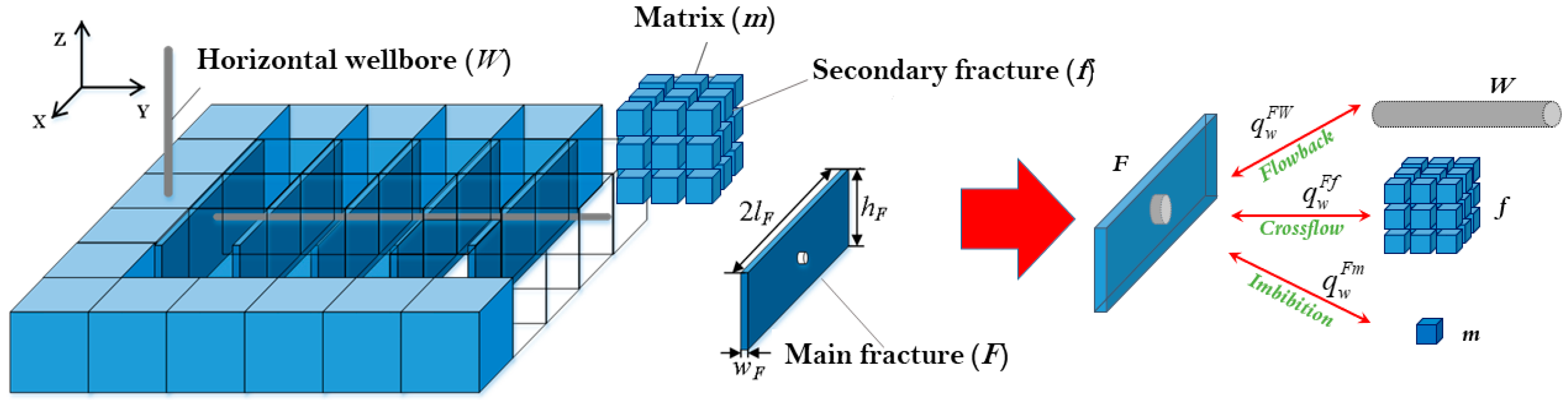
3.1. Physical Assumptions

Based on the above flow mechanism model, a multiple-porosity system for simulating fracturing-fluid hydrodynamic equilibrium is proposed as shown in Figure 2. The multiple-porosity physical model is composed of four interconnected domains, i.e., wellbore (W), main fractures (F), secondary fractures (f) and matrix (m). The classic dual-porosity model is used to describe the f and m [11,12], which are both connected with F. Taking the F as a kernel, all of the flow into and out of the other three domains can be treated as source-sink terms, i.e., q^WF, q^Ff, q^Fm.

For modeling the hydrodynamic equilibrium process, the following assumptions were made: (1) Two-dimensional flow is considered and gravity is ignored; (2) The crossflow in NF is considered to be a Darcy flow (Equation (1)); (3) The flow in F is considered to be a high-velocity non-Darcy flow, although actually this assumption is only valid for the transient moment when the main fractures are open; (4) The imbibition into m is driven by the chemical potential difference (Equation (2)); (5) The gas flow (including convection, diffusion and adsorption) within the multiple-porosity system is considered; (6) Pressure-dependent porosity is considered in F and f; (7) Wellbore is considered as a source-sink term in the center of F without compressibility; and (8) Fluid is slightly compressible.

3.2. Hydrodynamic Equation of Fracturing-Fluids

The mass balance equation for the fracturing-fluid flow in main fractures is expressed below

$$\frac{\partial ({\rho }_w{\varphi }^F{S}_w^F)}{\partial t_s}=-\nabla \left({\rho }_w{v}_w^F\right)+q_w^{WF}-q_w^{Ff}-q_w^{Fm}$$

(3)

where the term on the left, $\partial ({\rho }_w{\varphi }^F{S}_w^F)/\partial t_s$, refers to the mass variation in F, including the product of fracturing-fluid density ${\rho }_w$, saturation $S_w^F$, and main fracture porosity ${\varphi }^F$ change with shut-in time t_s, while the first term on the right side, $\nabla \left({\rho }_w{v}_w^F\right)$, refers to the fracturing-fluid flux term in F, which is related to the fracturing-fluid flow velocity ${\nu }_w^F$. Due to the high conductivity of F, the following non-Darcy flow equation was used [13]

$$-\nabla p_w^F=\frac{{\eta }_w}{k^F{k}_{rw}^F}{v}_w^F+\beta {\rho }_w{\left(v_w^F\right)}^2$$

(4)

where $p_w^F$ refers to the pore pressure in F; $k^F$ refers to the main fracture’s permeability; $k_{rw}$ refers to the relative permeability of fracturing-fluids; ${\eta }_w$ refers to the viscosity of fracturing-fluids; and $\beta$ denotes the non-Darcy coefficient.

Further, the second term in Equation (3) on the right side, $q_w^{FW}$, refers to the wellbore–fracture flux term, which is zero during well shut-in, and becomes the flowback rate during production. This flux term is driven by the hydraulic pressure difference, which is defined by Bian et al. [14] as follows:

$$q_w^{WF}=\frac{{\alpha }_1{\rho }_w{k}^F{k}_{rw}\left(p_w^W-p_{{}_w}^F\right)}{{\eta }_w{B}_w}.$$

(5)

The third term in Equation (3) on the right side, $q_w^{Ff}$, refers to the crossflow term between the main fracture and the secondary fracture, which is also driven by the hydraulic pressure difference and derived from Kazemi’s model [15]:

$$q_w^{Ff}=\frac{{\alpha }_2{\rho }_w{k}^F{k}_{rw}^F}{{\eta }_w}\left(p_w^F-p_w^f\right).$$

(6)

Likewise, the remaining term in Equation (3) on the right side, $q_w^{Fm}$, refers to the imbibition term from the hydraulic fracture network to the matrix, which is defined by [9]

$$q_w^{Fm}=\frac{{\alpha }_3{\rho }_w{k}^F{k}_{rw}^F}{{\eta }_w}\left(p_w^F-p_w^m+p_{c,w}^F-p_{c,w}^m+p_{\pi }\right)$$

(7)

where $p_{c,w}$ refers to the liquid-phase capillary pressure, since the gas–liquid two phase flow is considered; and $p_{\pi }$ refers to the osmotic pressure, which is derived from Marine and Fritz’s equation [16]:

$$P_{\pi }=\lambda \frac{RT}{V_w}\ln \frac{x_w^F}{x_w^m}.$$

(8)

The three shape factors, ${\alpha }_1,{\alpha }_2,{\alpha }_3$ represent the transmission between F and the other three domains in Equations (5)–(7), respectively. The derivation can be found in Appendix 1 in Wang et al. [9].

3.3. Model Solution

The semi-implicit finite difference scheme was used to solve the mass conservation and flux equations, including equation discretization, transmissibility calculation, introducing initial and boundary conditions, variable calculation and loop iteration. The semi-implicit finite difference algorithm is not new, and the details can be found in any reference book of computational mathematics.

4. Hydrodynamic Equilibrium Simulation

4.1. Description of the Simulation Model

Numerical simulation of the hydrodynamic equilibrium process in a reservoir was performed using our developed simulation programming based on the developed mathematical model. In this study, a fifteen-stage, hydraulically fractured horizontal well with a lateral length of 1350 m located in the centre of a shale reservoir (1500 m × 560 m × 40 m) was considered. Each single stage creates three transverse main fractures along the horizontal wellbore with a fracture spacing of 30 m (x_f = 30 m). All of the main hydraulic fractures (n^F = 45) were assumed to be identical, as shown in Figure 3. The water–gas relative permeability and capillary pressure curves for F, f and m were assigned according to reference values [17,18]. The input reservoir and hydraulic fracture parameters of the simulation model are listed in

Table 1. The input reservoir and hydraulic fracture parameters of the simulation model [7,8,19,20,21,22,23,24,25].

Variable, Symbol	Value	Variable, Symbol	Value
Main fracture half-length	140 m	Rock compressibility	4.4 × 10−4 MPa−1
Main fracture conductivity	2D·cm	Gas compressibility	0.03 MPa−1
Main fracture porosity	0.15	Membrane efficiency	0.3
Matrix permeability	10−4 mD	Gas density at standard condition	0.77 kg/m3
Matrix porosity	0.05	Fracturing-fluid density	1000 kg/m3
Secondary fracture permeability	0.01 mD	Source rock density	2560 kg/m3
Secondary fracture porosity	0.015	Initial reservoir pressure	25 MPa
Fracturing-fluid compressibility	5 × 10−4 MPa−1	Gas viscosity	0.058 mPa·s
Main fracture closure coefficient	0.05 MPa−1	Secondary fracture closure coefficient	0.032 MPa−1
Partial molar volume of water	18.02 × 10−6 m3/mol	Shape factor α1, α2, α3	300 m−2, 3 m−2, 0.3 m−2
Fracturing-fluid salinity	1000 ppm	Fracturing-fluid viscosity	0.8 mPa·s
Matrix salinity	280,000 ppm	Initial water saturation	0.2

.

The fracturing-fluid pumping was simulated as a water-injection process. The hydrodynamic equilibrium simulation was initialized by continuously injecting fracturing-fluid for 2 h into the horizontal wellbore and following a well shut-in of 60 days. The bottom-hole flowing pressure during the pumping was set to 55 MPa, and the total pumping volume was 8150 m³. The post-shut-in production was simulated at a bottom-hole flowing pressure of 5 MPa.

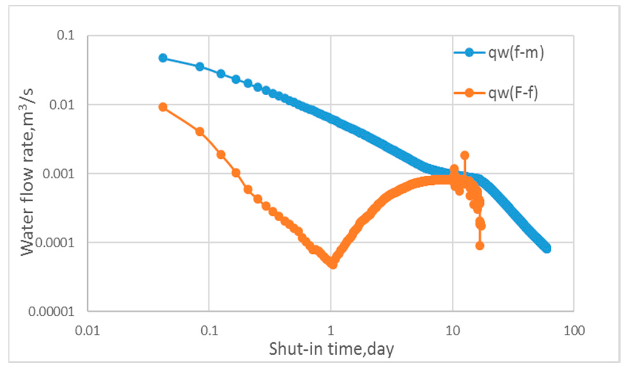
4.2. Simulation Results

Figure 4 displays the simulated bottom-hole flowing pressure during the well shut-in process. It indicates that the bottom-hole flowing pressure has decreased to 28 MPa after 1 day of shut-in, and this value lasts for the next 59 days. This big pressure drop during the initial 1 day of shut-in is consistent with field observations, which are believed to be caused by fracturing-fluid leakoff, hydraulic-fracture closure and proppant recompaction [26,27,28]. Figure 5 displays the pore pressure profiles in the hydraulic fracture network during the well shut-in process. In Figure 5, the coordinate-axis x represents the location along the main hydraulic-fracture plane. The coordinate-axis y represents the pore pressure. The zero point of axis x and axis y represents the location of the wellbore and the center of the main hydraulic fracture. The simulation result indicates that there are two zones in the fracture network, i.e., an inner zone of 140 m adjacent to the coordinate origin (the fracture part), and an outer zone 140 m away from the coordinate origin (the matrix part). With the increase in shut-in time, the pore pressure in the inner zone decreased, but the pore pressure in the outer zone increased, indicating that the energy spread happened from hydraulic fracture to formation during the shut-in periods. Moreover, like the wellbore pressure drop, the initial 1 day of shut-in made the hydraulic fracture release the most pressure.

Figure 6 and Figure 7 respectively display the evolution of fracture network crossflow and matrix imbibition profiles during the shut-in process. The simulation result indicates that, during the well shut-in process, the fracture system discharges water (as shown in Figure 6, the water saturation profile decreases with the shut-in time), while the matrix system sucks water in (as shown in Figure 7, the water saturation profile increases with the shut-in time). The decrease in water saturation in the main fracture occurs more quickly than the increase in that in the matrix due to the higher conductivity of secondary fractures.

Figure 8 indicates that the imbibition from the hydraulic fracture network into the shale matrix does not cease within 60 days, although the imbibition flux value becomes very small. The crossflow with the hydraulic fracture network ceases at 17 days of well shut-in, indicating that the hydraulic fracture system achieves hydrodynamic equilibrium. Moreover, the crossflow rate in the hydraulic fracture system shows a sag at the time of 1 day of shut-in. That is consistent with the biggest pressure drop in the fracture network during the 1-day shut-in, shown in Figure 4 and Figure 5, indicating the hydraulic fracture’s closure.

Figure 9 exhibits the increasing imbibition volume from the fracture system to the matrix system with the shut-in time. The simulation result indicates that the hydraulic pressure is the dominant imbibition driving force, while the chemical osmosis and capillarity show small effects on the fracturing-fluid imbibition. Specifically, after 60 days of well shut-in, the accumulated imbibition volume from the hydraulic fracture network to the shale matrix is 4165 m³, which is 51.1% of the injected fluid volume. Capillarity-induced imbibition and osmosis-induced imbibition comprised 19.4% and 12.4% of the volume, respectively.

5. Shut-In Time Optimization

5.1. Shut-In Time Determination

Figure 10 shows the simulated water load recovery and gas production in 30 days with different shut-in times. Seen as a whole, with the extension of the shut-in time, the cumulative gas production increases and the water load recovery decreases. Concretely, there are two inflection points in the cumulative gas production curve, when the shut-in time t_s is 1 day and 17 days, respectively. The first inflection point, i.e., t_s = 1 day, corresponds to the elastic closure time of hydraulic fractures. The second inflection point, i.e., t_s = 17 days, corresponds to the crossflow equilibrium time in a hydraulic fracture network. Based on the simulation results, the crossflow equilibrium time of 17 days can be used for the optimal shut-in time’s determination, because this is the most time-effective point for pursuing the production rate if the corresponding fracturing-fluid loss is allowable.

5.2. Shut-In Time Sensitivity

The simulation results indicate that the hydrodynamic equilibrium time of the hydraulic fracture system (the crossflow equilibrium time) coincides with the optimal shut-in time. A simulation of the crossflow equilibrium time’s sensitivity to different reservoir and fracture properties can guide the shut-in time determination for different field conditions. Figure 11, Figure 12 and Figure 13 show the simulated crossflow equilibrium time (also the optimal shut-in time) under different imbibition conditions. The three imbibition driving forces, i.e., P_c, P_h and P_π, are represented by a capillary pressure multiplier (P_c/P_{c_base}, injection pressure and membrane efficiency (λ) respectively). Figure 14 shows the simulated crossflow equilibrium time (also the optimal shut-in time) under different hydraulic fracture conductivities.

The results show that the optimal well shut-in time is positively correlated with the injection pressure and hydraulic fracture conductivity, although the correlation degree between them is different. That means a higher initial reservoir pressure (corresponding to a lower injection pressure) needs a shorter shut-in. The optimal well shut-in time is negatively correlated with the capillary pressure. That means a higher capillary pressure (corresponding to a strong water-wet reservoir) needs a shorter shut-in. The chemical osmosis also seems to affect the well shut-in only within a certain range of rock osmosis properties, in this simulation case with λ from 0.1 to 0.5. Taken together, the sensitivity simulation results indicate that a strong water-wet and high initial pressure shale gas reservoir with a low conductivity of hydraulic fracture needs a shorter well shut-in time. In contrast, a weak water-wet and low initial pressure shale gas reservoir with a high conductivity of hydraulic fracture needs a longer well shut-in time.

6. Discussion

In practice, the well shut-in time has become a concern in recent years because it has proven to be involved in the post-fracturing production of shale gas wells. Meanwhile, complicated reservoir hydrodynamic problems, such as fracturing-fluid imbibition from the milli-scale fracture system to the nano-scale matrix, have arisen due to the practical technical routine of the application of hydraulic fracturing treatments in shale gas reservoirs. However, the study of well-reservoir relevance is limited in the previous research.

Our intention for this study was to establish a relation between the hydrodynamic equilibrium mechanism in a reservoir and the well production schedule (the optimal shut-in time) with our mathematical model and numerical simulation tool. The developed mathematical model considers the fracturing-fluid imbibition mechanism (P_h + P_c + P_π) and a W-F-f-m coupled multiple-pore structure. The hydrodynamic equilibrium time of the fracture system (the crossflow equilibrium time) was calculated by simulation of fracture-network crossflow and matrix imbibition during an extended well shut-in period. This crossflow equilibrium time was found to coincide with the most time-effective well shut-in time through a large number of numerical simulations of different shut-in-production schedules. At this point, the link between reservoir and well emerges. The crossflow equilibrium time can be used to determine the optimal well shut-in time.

Further sensitivity studies for investigating the effect of different reservoir and fracture properties on the crossflow equilibrium time aimed to provide a general guide for shut-in time determination under different field conditions. For example, the simulation results indicate that strong water-wet and high-pressure shale gas reservoirs, once stimulated by hydraulic fracturing and generating low-conductivity fractures, do not need a long shut-in time. The optimal shut-in time range is from 100 h to 900 h for the current simulation cases, in which the optimal shut-in time of the base case is 408 h (17 days). The limited number of variables and single-variable sensitivity analysis are limitations of the present study. A comprehensive multivariable analysis based on the specific reservoir and fracturing treatment conditions will be the subject of future work.

7. Conclusions

(1)

After 60 days of well shut-in, the accumulated imbibition volume of fracturing-fluid from the hydraulic fracture network to the shale matrix is 4165 m³, which is 51.1% of the injected fluid volume. Capillarity-induced imbibition and osmosis-induced imbibition comprised 19.4% and 12.4% of the volume, respectively.

(2)

The imbibition from the hydraulic fracture network into the shale matrix did not cease within 60 days, although the imbibition flux value became very small. The crossflow with the hydraulic fracture network ceases at 17 days of well shut-in, indicating that the hydraulic fracture system achieved hydrodynamic equilibrium.

(3)

The hydrodynamic equilibrium time of the hydraulic fracture system happened to coincide with the inflection point of the incremental curve of post-fracturing production with shut-in time. This time point can be the optimal shut-in time if the corresponding fracturing-fluid loss is allowed.

(4)

The optimal well shut-in time is different for different imbibition driving force conditions, including the degree and regularity of influence. So, the optimal well shut-in schedule should be determined based on the specific reservoir and fracturing treatment conditions.

(5)

The simulation results indicate that a strong water-wet and high initial pressure shale gas reservoir with a low conductivity of hydraulic fracture needs a shorter well shut-in time. In contrast, a weak water-wet and low initial pressure shale gas reservoir with a high conductivity of hydraulic fracture needs a longer well shut-in time.

References

1. Wattenbarger, R.A.; Alkouh, A.B. New Advances in Shale Reservoir Analysis Using Flowback Data. In Proceedings of the SPE Eastern Regional Meeting, Pittsburgh, PA, USA, 20–22 August 2013. [Google Scholar]
2. Adefidipe, O.A.; Dehghanpour, H.; Virues, C.J. Immediate Gas Production from Shale Gas Wells: A Two-Phase Flowback Model. In SPE-168982. In Proceedings of the SPE Unconventional Resources Conference, The Woodlands, TX, USA, 1–3 April 2014. [Google Scholar]
3. Satyanarayana Gupta, D.V.; Valko, P. Fracturing Fluids and Formation Damage. In Modern Fracturing-Enhancing Natural Gas Production; Economides, M.J., Martin, T., Eds.; Energy Tribune Publishing: Houston, TX, USA, 2007. [Google Scholar]
4. Dutta, R.; Lee, C.H.; Odumabo, S. Experimental Investigation of Fracturing-Fluid Migration Caused by Spontaneous Imbibition in Fractured Low-Permeability Sands. SPE Reserv. Eval. Eng. 2014, 17, 74–81. [Google Scholar] [CrossRef]
5. Wang, M.; Leung, J.Y. Numerical investigation of fluid-loss mechanisms during hydraulic fracturing flow-back operations in tight reservoirs. J. Pet. Sci. Eng. 2015, 133, 85–102. [Google Scholar] [CrossRef]
6. Ghanbari, E.; Dehghanpour, H. The fate of fracturing water: A field and simulation study. Fuel 2016, 163, 282–294. [Google Scholar] [CrossRef]
7. Wang, F.; Pan, Z.; Zhang, S. Modeling Water Leak-off Behavior in Hydraulically Fractured Gas Shale under Multi-mechanism Dominated Conditions. Transp. Porous Media 2017, 118, 177–200. [Google Scholar] [CrossRef]
8. Perapon, F. Managing shut-in time to enhance gas flow rate in hydraulic fractured shale reservoirs: A simulation study. In Proceedings of the SPE Annual Technical Conference and Exhibition, New Orleans, LA, USA, 30 September–2 October 2013. [Google Scholar]
9. Wang, F.; Pan, Z.; Zhang, S. Impact of chemical osmosis on water leakoff and flowback behavior from hydraulically fractured gas shale. J. Pet. Sci. Eng. 2017, 151, 264–274. [Google Scholar] [CrossRef]
10. Meng, M.; Ge, H.; Ji, W.; Shen, Y.; Su, S. Monitor the process of shale spontaneous imbibition in co-current and counter-current displacing gas by using low field nuclear magnetic resonance method. J. Nat. Gas Sci. Eng. 2015, 27, 336–345. [Google Scholar] [CrossRef]
11. Gilman, J.R. Practical Aspects of Simulation of Fractured Reservoirs. In Proceedings of the International Forum on Reservoir Simulation, Buhl, Germany, 23–27 June 2003. [Google Scholar]
12. Yan, B.; Mi, L.; Wang, Y. Mechanistic Simulation Workflow in Shale Gas Reservoirs. In Proceedings of the SPE Reservoir Simulation Conference, Montgomery, TX, USA, 20–22 February 2017. [Google Scholar]
13. Bybee, K. Non-Darcy Flow in Hydraulic Fractures. J. Pet. Technol. 2006, 58, 58–59. [Google Scholar] [CrossRef]
14. Bian, X.; Zhang, S.; Zhang, J.; Wang, F. A New Method to Optimize the Fracture Geometry of a Frac-packed Well in Unconsolidated Sandstone Heavily Oil Reservoirs. Sci. China Technol. Sci. 2012, 55, 1725–1731. [Google Scholar] [CrossRef]
15. Kazemi, H.; Gilmanc, J.R.; Elsharkawy, A.M. Analytical and Numerical Solution of Oil Recovery From Fractured Reservoirs With Empirical Transfer Functions. SPE Reserv. Eng. 1992, 7, 219–227. [Google Scholar] [CrossRef]
16. Marine, I.W.; Fritz, S.J. Osmotic Model to Explain Anomalous Hydraulic Heads. Water Resour. Res. 1981, 17, 73–82. [Google Scholar] [CrossRef]
17. Zhang, T.; Li, X.; Li, J.; Feng, D.; Li, P.; Zhang, Z.; Chen, Y.; Wang, S. Numerical investigation of the well shut-in and fracture uncertainty on fluid-loss and production performance in gas-shale reservoirs. J. Nat. Gas Sci. Eng. 2017, 46, 421–435. [Google Scholar] [CrossRef]
18. Jurus, W.J.; Whitson, C.H.; Golan, M. Modeling water flow in hydraulically-fractured shale wells. In Proceedings of the SPE Annual Technical Conference and Exhibition, New Orleans, LA, USA, 30 September–2 October 2013. [Google Scholar]
19. Garavito, A.M.; Kooi, H.; Neuzil, C.E. Numerical modeling of a long-term in situ chemical osmosis experiment in the Pierre Shale, South Dakota. Adv. Water Resour. 2006, 29, 481–492. [Google Scholar] [CrossRef]
20. Gdansk, R.D.; Fulton, D.D.; Chen, C. Fracture-face-skin evolution during cleanup. SPE Prod. Oper. 2009, 24, 22–34. [Google Scholar] [CrossRef]
21. Dacy, J.M. Core tests for relative permeability of unconventional gas reservoirs. In Proceedings of the SPE Annual Technical Conference and Exhibition, Florence, Italy, 19–22 September 2010. [Google Scholar]
22. Chen, Z.; Xue, C.; Jiang, T.; Qin, Y. Proposals for The Application of Fracturing by Stimulated Reservoir Volume (SRV) in Shale Gas Wells in China. Nat. Gas Ind. 2010, 30, 30–32. [Google Scholar]
23. Zheng, L.; Samper, J.; Montenegro, L. A coupled THC model of the FEBEX in Situ Test with Bentonite Swelling and Chemical and Thermal Osmosis. J. Contam. Hydrol. 2011, 126, 45–60. [Google Scholar] [CrossRef] [PubMed] [Green Version]
24. Eshkalak, M.O.; Aybar, U.; Sepehrnoori, K. An Integrated Reservoir Model for Unconventional Resources, Coupling Pressure Dependent Phenomena. In Proceedings of the Presented at the SPE Eastern Regional Meeting, Charleston, WV, USA, 21–23 October 2014. [Google Scholar]
25. Wang, F.; Li, B.; Chen, Q.; Zhang, S. Simulation of Proppant Distribution in Hydraulically Fractured Shale Network during Shut-in Periods. J. Pet. Sci. Eng. 2019, 178, 467–474. [Google Scholar] [CrossRef]
26. Ehlig-Economides, C.A.; Ahmed, I.A.; Apiwathanasorn, S.; Lightner, J.H.; Song, B.; Vera Rosales, F.E.; Xue, H.; Zhang, Y. Stimulated Shale Volume Characterization: Multiwell Case Study from the Horn River Shale: II. Flow Perspective. In SPE Annual Technical Conference and Exhibition; Society of Petroleum Engineers: San Antonio, TX, USA, 2012. [Google Scholar]
27. Huang, X.; Wang, J.; Chen, S.; Gates, I.D. A simple dilation-recompaction model for hydraulic fracturing. J. Unconv. Oil Gas Resour. 2016, 16, 62–75. [Google Scholar] [CrossRef]
28. Liu, Y.; Guo, J.; Chen, Z. Leakoff characteristics and an equivalent leakoff coefficient in fractured tight gas reservoirs. J. Nat. Gas Sci. Eng. 2016, 31, 603–611. [Google Scholar] [CrossRef]
Figure 1. Schematic of fracturing-fluid hydrodynamic equilibrium during the shut-in process.
Energies 13 00961 g001
Figure 2. Physical model for the fracturing-fluid hydrodynamic equilibrium simulation.
Energies 13 00961 g002
Figure 3. Schematic of the simulation model.
Energies 13 00961 g003
Figure 4. Decrease in bottom-hole flowing pressure.
Energies 13 00961 g004
Figure 5. Pore pressure profiles in the fracture network during well shut-in.
Energies 13 00961 g005
Figure 6. Crossflow profiles in the fracture network during well shut-in.
Energies 13 00961 g006
Figure 7. Imbibition profiles in the matrix during well shut-in.
Energies 13 00961 g007
Figure 8. Imbibition flux and imbibition equilibrium with shut-in time.
Energies 13 00961 g008
Figure 9. Imbibition volumes with different driving forces.
Energies 13 00961 g009
Figure 10. Shut-in optimization curve for the base case.
Energies 13 00961 g010
Figure 11. Shut-in optimization curve for different Pc.
Energies 13 00961 g011
Figure 12. Shut-in optimization curve for different Ph.
Energies 13 00961 g012
Figure 13. Shut-in optimization curve for different Pπ.
Energies 13 00961 g013
Figure 14. Shut-in optimization curve for different Fc.
Energies 13 00961 g014