Abstract
The definition of appropriate energy targets for large industrial processes is a difficult task since operability, safety and plant layout aspects represent important limitations to direct process integration. The role of heat exchange limitations in the definition of appropriate energy targets for large process sites was studied in this work. A computational framework was used which allows to estimate the optimal distribution of process stream heat loads in different subsystems and to select and size a site wide utility system. A complex Swedish refinery site is used as a case study. Various system aggregations, representing different patterns of heat exchange limitations between process units and utility configurations were explored to identify trade-offs and bottlenecks for energy saving opportunities. The results show that in spite of the aforementioned limitations direct heat integration still plays a significant role for the refinery energy efficiency. For example, the targeted hot utility demand is reduced by 50–65% by allowing process-to-process heat exchange within process units even when a steam utility system is available for indirect heat recovery. Furthermore, it was found that direct process heat integration is motivated primarily at process unit level, since the heat savings that can be achieved by allowing direct heat recovery between adjacent process units (25–42%) are in the same range as those that can be obtained by combining unit process-to-process integration with site-wide indirect heat recovery via the steam system (27–42%).
1. Introduction
Energy targeting is typically performed in the early stages of chemical process design in which the minimum energy requirement (MER) of the process is estimated [1]. To set targets in the early stages of design is essential to develop processes that use as little energy as is economically reasonable. Pinch methodology was designed to achieve this goal, and is also expected to be used for this purpose in future developments [2]. In complex thermal systems, knowing the minimum theoretical heat demand that has to be provided by an external source (hot utility) can be of great help for the engineer for guiding process design [3]. Setting targets for heat recovery is an important step also in retrofit situations [4] in order to estimate the potential energy savings that can be achieved by rearranging and modifying the existing heat exchange network.
In large industrial processes, plant layout, operability, and safety issues usually place substantial limitations to achieving maximum heat integration across the complete site. For example, Chew et al. [5] discussed implementation issues for heat integration in industrial sites and Svensson et al. [6] reviewed the literature on operability related to integrated biorefineries. Undoubtedly, implementation and operability issues makes the estimation of relevant energy targets a difficult task.
Oil refineries and petrochemical plants are among the cases in which these aspects are more apparent. In an oil refinery, direct heat integration, for instance, between the crude distillation unit and the downstream product upgrading units is difficult as it could hinder reliable refinery operation. In addition, different process units are designed and built by different technology providers and may be subject to revamping and retrofit at different moments of the plant life, which significantly limits direct heat integration between units. An overview of operability issues related to heat recovery retrofits in oil refineries is recently presented by Marton et al. [7].
For the reasons discussed above, the MER target calculated for the complete set of thermal streams for a complex process system is not a useful reference for engineering practice. Consequently, many Heat Integration studies for large refinery sites focus on heat recovery within specific process refinery parts or even a few, single process units rather than across the whole site. For instance, Al-Riyami et al. [8] used pinch analysis insights and economic analysis to investigate in detail possible HEN retrofit options for a fluid catalytic cracker (FCC). The FCC plant was also the focus of the work of Al-Mutairi [9], who introduced a new energy targeting approach for dealing with variations in flowrates and temperatures, as a first step for designing an optimal and flexible heat exchanger retrofit. Dinçer and Şentarli [10] used pinch analysis to identify opportunities for increased heat recovery within the crude distillation unit (CDU) in a Turkish refinery. Energy targeting for the CDU was also investigated by Ji and Bagajewicz [11]. The CDU is one of the largest energy consumption units in a refinery, and the crude preheating section is a particularly challenging heat exchanger network problem in which operability is a crucial aspect, given that extensive stream splitting is often required for reaching significant energy savings. A CDU was also analysed for retrofit opportunities by Yimyam and Siemanond [12]. Recently, Cui and Sun [13] used pinch analysis to assess opportunities for heat integration between currently separate preheating sections for crude distillation. Goodarzvand-Chegini et al. [14] instead investigated retrofitting opportunities in the hydrocracking process, which is of special interest due to high pressure levels, which impose challenging constraints on operation and plant equipment. Walmsley et al. [15] recently suggested a promising approach for automated energy targeting in retrofit situations, and applied it to a large-scale refinery case study. However, in all studies cited above, only direct process heat exchange was considered.
In order to avoid difficulties related to direct heat integration between process units, a heat distribution and heat collection system, such as steam network, is often the most practical way to deal with site-wide heat integration at refineries or in large chemical complexes. To target opportunities for site-wide heat integration via steam utility systems, the concept of total site analysis (TSA) was developed. The first attempts made by Dhole and Linnhoff [16], were further developed into a comprehensive methodology with a range of demonstrated applications [17]. A review of state-of-the-art in total site heat integration methodology was presented by Liew et al. [18]. Recent developments to the TSHI method include, for example, a method for total site integration of trigeneration systems [19].
In traditional TSHI approaches, specific process parts of the plant (subsystems) can only exchange heat via utility systems and self-sufficient heat pockets in the heat cascades of individual subsystems are not utilized for site-wide heat integration. Heat pockets are also discarded in recent developments of TSHI targeting approaches that consider isothermal as well as non-isothermal utilities in the same targeting method [20]. Starting from the basic case of two plants [21], Bagajewicz and Rodera tackled this issue by developing a general model for heat transfer between process plants via intermediate heat transfer fluids and proposed a procedure for integration of the heat transfer loops [22]. Bagajewicz and Rodera [23], also proposed a heat belt for the heat transfer between plants. However, the general model becomes non-linear if more than three separate plants are considered, which motivates a different approach for more complex sites. Bandyopadhyay et al. [24] introduced the site level grand composite curves for indirect heat transfer. They proposed a methodology for cogeneration targeting at the site level, a topic that is extensively covered in literature. Two other recent examples, where refineries are used as case studies, are given by Ghannadzadeh et al. [25] and Ren et al. [26]. Indirect heat transfer was also considered by Stijepovic and Linke [27], who extended the concept to industrial clusters with multiple process plants. The optimal operation and retrofit design of a steam utility system is by itself a difficult task, as demonstrated, for instance, in two recent examples related to petroleum refineries [28] and total sites [29]. In all the total site studies cited above, it is mainly the utility system that is optimized, and heat is assumed to be transferred between process plants via steam lines or other site-wide heat transfer loops.
Since almost all the process units in a refinery are connected to a steam utility system, increased heat recovery in a single unit is likely to affect the site’s overall steam balances and thereby indirectly the fuel consumption in steam boilers in addition to direct reduction of fuel consumption in local furnaces [30]. To what extent a local improvement translates into fuel savings at the site-wide level depends highly on the steam network features. Local unit heat integration opportunities and site wide integration via a steam network are therefore necessarily intertwined and should be considered simultaneously when estimating the fuel savings consequences from increased heat recovery at a large process site. Zhang et al. [31] proposed a more hierarchical approach, which is an attempt in this direction. Their proposed methodology was demonstrated for a refinery site, but with a lack of details regarding the individual methodological steps. Wang et al. [32] proposed a method for combining direct and indirect heat integration for multiple plants, selecting one suitable process stream with large duty which is used to directly transfer heat from one plant to another and, furthermore, considering only the current heat surplus and deficits of the individual plants. Becker and Maréchal [33] proposed an extension of previous work [34], in which they consider both direct heat exchange within subsystems and indirect heat recovery between subsystems via heat transfer systems in the targeting phase. The heat transfer systems may include heat-only steam networks, heat recovery loops as well as co-generation systems. In their approach, however, direct heat exchange between subsystems is not allowed.
As shown by the above literature review, there are many examples of heat integration studies in oil refineries (or other complex chemical processing sites), in which energy targets are estimated. State-of-the-art methodology typically consider direct heat integration within limited areas of the process and site-wide integration via a heat collection and distribution system. However, none of the studies cited above systematically investigate the role of system aggregation by studying the impact on site energy targets of accepting successively larger (more aggregated) subsystems. Such different system aggregation levels may include direct heat integration within process units and site-wide integration via utility systems, but may also include more complex patterns of heat exchange restrictions, for example, where some degree of cross-unit heat recovery can be achieved via direct heat exchange between certain units (e.g., adjacent process units and plant areas). Consequently, there is a lack of knowledge regarding the trade-offs between direct process heat integration within and across process units and site-wide heat recovery via a steam utility system.
Thus, the objective of this paper is to systematically study how different levels of system aggregation (i.e., different levels of restrictions for process-to-process, and process-to-utility heat exchange) affect the heat recovery and co-generation targets for a large complex industrial process site. In this regard, different values of the minimum temperature difference allowed for heat exchange is an important design parameter that affects the invested heat exchange area.
With the proposed approach, alternative solutions for reaching a given MER target can be identified, considering different types of restrictions for direct heat exchange in combination with minimum allowable temperature difference for heat exchanging. In this way, important insights can be reached regarding the aspects that should be pursued to improve the site heat recovery by: a) improving process direct heat integration by allowing matching between process thermal streams in larger aggregated subsystems; b) improving the process indirect heat transfer by means of more advanced steam network layouts; c) identifying reasonable minimum temperature differences for heat exchange. The proposed approach can be used to identify realistic heat integration targets for complex process sites.
The systematic investigation of various types of constraints for direct heat integration is enabled by the application of a calculation framework developed to automatically generate the required set of model equations. The advantages of the proposed approach is demonstrated on a case study of a refinery on the west coast of Sweden.
2. Materials and Methods
The energy targeting problem is solved using a computational framework for constrained heat integration targeting that allows for exploring different levels and patterns of heat exchange restrictions for large process sites. For this purpose, two categories of system aggregation are introduced. Process-to-process aggregation refers to the level of subdivision of the process thermal streams into units and to the various patterns of restriction of process-to-process direct heat transfer. Process-to-utility aggregation refers to the complexity of the utility system and possible restrictions to heat exchange between process and utility streams.
Section 2.1 introduces the mathematical modelling framework applied in the analysis. Section 2.2 then presents the refinery case study. For the case study, different cases of process-to-process and process-to-utility aggregation are defined in Section 2.3, and the case study-specific objective function of the optimization problem is then presented in Section 2.4.
2.1. Mathematical Modelling Framework for Constrained Heat Integration
At a given process site it is possible to identify sets of thermal streams within which heat can be exchanged without limitations. In this work, such subsets of process thermal streams are referred to as process “units”. Typically, these are streams that belong to the same process plant or production area, or that are grouped together based on operability considerations. However, thermal streams belonging to one unit may be allowed to exchange heat directly with thermal streams from certain other process units, such as neighbouring process plants. This implies that certain process streams can be considered as candidates for the heat cascade of more than one process units, partially or fully. Consequently, a “unit” is not necessarily equivalent to an “independent heat cascade” and in this sense a unit is different from what other authors refer to as “areas of integrity” [35], “zones” [36] or “subsystems” [33].
The number of process units and the patterns of heat exchange restrictions between the units define the size and number of subsystems, which may be treated as separate heat cascades. The system aggregation thereby affects the degree of heat integration, that is, the amount of heat that is exchanged between process streams directly or indirectly.
For a specific process site, it is possible to qualitatively identify relevant levels of process-to-process aggregation (i.e., individual process plants, process areas based on site layout, groups of thermal streams between which there are no heat exchange limitations, etc.) and relevant layouts of utility systems that can achieve different levels of heat integration. Section 2.3.1 describes the different patterns of heat exchange within and between process units considered in this work. Such information can then be translated to constraints for the heat cascade optimization and utility targeting. More explicitly, for streams that may exchange heat between different units, and which therefore may participate in different heat cascades, a model is needed to determine the optimal distribution of the heat load of the stream between the potential heat cascades.
In this work, graph theory insights are used to formulate the appropriate heat cascade constraints (see Appendix A for more details about model formulation). With this approach, subsystems that can be handled as separate heat cascades and that can include more than one unit can be identified by automated procedures [37]. Thereby, the mathematical constraints used in the energy targeting analysis can be generated automatically. This allows for substantial simplification of the model formulation, since the user only needs to specify how heat exchange is allowed and does not need to explicitly formulate the constraints representing the individual heat cascades.
Morandin [38] presents a simple example of a problem with heat exchange limitations in which the proposed methodology was applied to considering only fixed size units. However, the mathematical formulation also allows for including thermal units of variable size, such as steam networks and circulating water systems, which can be used for indirect heat transfer between different process units. The mathematical optimization framework is based on a linear programming (LP) approach in order to allow for simple solution strategies. Consequently, the different steam utility system configurations are modelled as a set of linear equations as proposed in previous work [39] and described in more detail in Appendix A. By combining heat exchange limitations and optimization of variable size units in the same model, the method incorporates elements of both zonal targeting and Total Site Analysis.
To summarize, the optimization framework can be used to address energy targeting problems with or without heat exchange restrictions including sizing of utility systems. The latter include the common problem of sizing a steam network with integrated steam cycles for Total Site Integration. The optimization problem was implemented in MATLAB (R2019b, The MathWorks Inc, Natick, MA, US). A calculation framework was developed that automatically builds the necessary sets of equations based on user input and solves the problem using a built-in LP solver. The user input includes a description of the different system units, the corresponding thermal streams and the neighbouring units with which heat exchange is possible. Additionally, the user may specify the different pressure levels and to a certain degree also different topologies of the site wide steam network.
2.2. The Refinery Case Study
The refinery considered here is located on the West coast of Sweden. It is a complex refinery with the capacity to process 11.4 Mtonnes of crude oil per year and is one of the most energy efficient refineries in Europe, according to the most recent Solomon refinery study published in 2018 [40]. An overview of the refinery is shown in Figure 1.
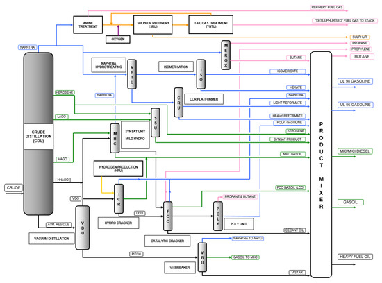
Figure 1.
Overview of the main material flows through the refinery processes. Adapted with permission from [41]; Copyright 2013, J.F. Brau.
Considerable efforts have been put into decreasing the environmental impact of the refinery process and motor fuel products, for instance by improving the conversion of difficult oil fractions and by extending the refinery to process biomass derived feedstocks, thereby increasing the renewable share in conventional motor fuels. Opportunities for CO2 mitigation have been investigated, including integration of large scale biomass gasification based biorefineries [42], or by integration of post-combustion CO2 capture technologies [43]. In parallel, energy targeting [44] and retrofit studies [45] have also been performed. In an on-going research project, operability aspects are being investigated for proposing more practical and relevant retrofit options [46].
In Figure 2, the process units are grouped into process areas, which fairly well represents the actual geographical layout of the site. The refinery consists of 16 process units, located in seven distinct areas which are separated by service roads. The units correspond to the main refinery process steps in which the crude oil undergoes distillation and the different hydrocarbon cuts are upgraded to final products. The refinery is therefore characterized by large material flows between units and areas. Direct process heat integration occurs primarily within each single unit. The role of process areas with respect to systems aggregation scenarios is presented in detail in Section 2.3.
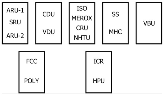
Figure 2.
Basic refinery layout showing the 16 process units and the seven distinct process areas. ARU: amine recovery; SRU: sulphur recovery (including the TGTU: Tall Gas Treatment Unit); CDU: crude distillation; VDU: vacuum distillation; ISO: isomerization; MEROX: mercaptan oxidation; CRU: catalytic cracking reforming; NHTU: naphtha hydrotreating; SS: Synsat; MHC: mild hydro cracker; VBU: Visbreaker; FCC: fluid catalytic cracker; POLY: polymerisation; ICR: hydrocracking; HPU: hydrogen production.
A steam network is used to collect and distribute heat between different units and areas [30]. Additional steam may be provided by steam boilers. Steam turbines for power production are also available. A simplified scheme of the steam system is shown in Figure 3.
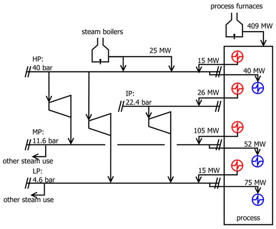
Figure 3.
Simplified layout of the steam utility system. Let down valves, steam drums, desuperheaters and other miscellaneous equipment are not shown. Red symbols indicate steam generation in process coolers, neglecting those used only for feed water heating and steam superheating. Blue symbols indicate process steam heaters. Indicated steam flows are rough estimates corresponding to current operation.
The stream temperatures and heat loads of the majority of the refinery heat exchangers were collected in 2008 with the help of process engineers [44]. Although the loads and temperatures of various process streams may vary during the year, and some refinery processes have changed, the data considered in this work is nevertheless fairly representative of the “current” situation. Overall 90 cold streams and 122 hot streams were identified which add up to a total of 212 thermal streams.
Based on the available measurements, the sum of the heat loads of all cold streams (total heat demand) is 1226 MW and the sum of the heat loads of all hot streams (total cooling demand) is 1372 MW. Currently, heat provided to process streams in process furnaces is 409 MW which means that 817 MW of heat are provided either by heat recovered by direct heat exchange between process streams or via the steam network. The heat delivered to the process by the steam network is 167 MW. This means that 650 MW corresponds to the heat recovered by direct process heat integration. A large share of the steam required for process heating is generated in process coolers. However, approximately 25 MW of high-pressure steam must be produced in steam utility boilers. Consequently, the total, current hot utility demand of the processes equals 434 MW (409 MW furnace heat + 25 MW high-pressure steam).
Note that in the refinery, steam is also required for direct injection in strippers, and for auxiliaries such as steam tracing, tank heating etc. This steam demand was not included in the process heat demand. Furthermore, steam is used in the refinery for power generation in steam turbines that drive pumps and compressors. Potential co-generation of power and steam for process heating is considered in the targeting analysis, but there is no constraint to ensure that this power generation is sufficient to drive all rotating equipment. Instead, it is assumed that these can either be driven by power co-generated with steam for non-process heating purposes (outside our system boundaries) or that these can be switched to electric motor drive if necessary, which is also possible in reality for the majority of these units. This implies that the targeted power co-generations is equivalent to replacing electricity from the grid.
2.3. Definition of Studied Cases
In the following sections, different levels of process-to-process aggregation are described by introducing different patterns of heat exchange restrictions between the refinery units. Process-to-utility aggregation is explored by considering different utility configurations which, for simplicity, are inspired by the current utility system.
2.3.1. Process-to-Process Aggregation: Definition of Relevant Cases of Direct Heat Exchange Limitations
There are two levels of process-to-process aggregation typically considered in energy targeting analysis: the unrestricted case in which heat exchange is allowed between all process streams without limitations, and the case in which direct heat exchange is allowed only within each single process unit; in the second case the total hot utility demand target is the sum of the process units hot utility demand targets.
Other cases are also worth investigating which allow direct heat exchange also between certain selected units, thereby representing different levels of system aggregation. In the case study, system aggregation levels are defined based on the process units, process areas, and geographical adjacency of the streams. The process areas here refer to the groups of process units located within the same geographical area bounded by the site’s service roads (Figure 2), while the geographical adjacency refers to the physical proximity between processes. Note that two process units may be adjacent (located close to each other) even if they are in separate areas (on separate sides of a service road), or they may be in the same area without being adjacent (e.g., if there is another process unit located between them in the same area). Since heat integration can be obtained by indirect heat transfer between units through the utility system, the case in which direct heat transfer is fully prohibited is also interesting.
For the studied refinery, the following cases were defined in order of increasing process-to-process aggregation:
- (a)
- No direct process heat integration possible
- (b)
- Direct heat integration possible only between streams within the same unit
- (c)
- Direct heat integration possible between adjacent units within the same area (Figure 4)
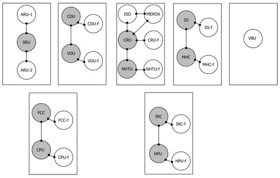 Figure 4. Graph illustrating allowed heat integration opportunities (indicated by edges between circles) when integration is allowed only between adjacent units within the same area (case c).
 - (d)
- Direct heat integration possible between adjacent units also across areas (Figure 5)
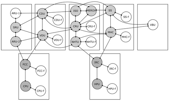 Figure 5. Graph illustrating allowed heat integration opportunities (indicated by edges between circles) when integration is allowed between adjacent units within the same area and as well as between adjacent areas (case d).
 - (e)
- Direct heat integration fully possible between all the units within same area only
- (f)
- Direct heat integration possible between adjacent areas (Figure 6)
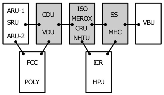 Figure 6. Graph illustrating allowed heat integration opportunities (indicated by edges between boxes) when direct heat integration is fully possible between all the units within the same area and heat integration is also possible between adjacent areas (case f).
 - (g)
- Unrestricted direct heat integration allowed between all site streams
Note that in the computational, graph-theory based framework (see Appendix A), adjacency represents allowed heat exchange between one unit and other units, and this may be defined based on any selected criteria. In case c), d) and f) above, adjacency refers to geographical proximity)
For the cases c) and d) in which unit-to-unit integration is allowed, it was decided that the streams above 250 °C are only allowed to exchange heat with other streams within the same unit, to take into account possible practical limitations of long piping distances for high temperature streams. This heat exchange limitation was imposed by grouping the portions of such streams above 250 °C into new virtual units denoted in Figure 4 and Figure 5 by the suffix “-f” (e.g., “CDU-f”) and by allowing such virtual units to be heat integrated only with the original process unit (e.g., CDU).
As explained in more detail in Section 2.1. and in Appendix A.2, information about the units with which heat exchange is allowed is given as input to the computational framework. In Figure 4, Figure 5 and Figure 6, allowed heat exchange between units (or areas) is indicated by edges between circles (boxes). This information is then used to automatically determine the relevant subsystems (independent heat cascades). For instance, if we consider Area 3 in Figure 4 (third area from the left in the top row), there are four subsystems within which all streams can exchange heat with each other: ISO/CRU/MEROX; CRU/CRU-f; CRU/NHTU; and NHTU/NHTU-f. Each of these subsystems represents an independent heat cascade. However, some units participate in more than one such heat cascade (for Area 3, these are the CRU and NHTU units). The heat load of streams from units that may participate in more than one heat cascade is distributed between the subsystems, and this is subject to optimization. In Figure 4, Figure 5 and Figure 6, shaded circles (or boxes) are used to represent such units for which the heat loads of steams should be distributed between different thermal cascades. The computational framework generates a set of linear inequality constraints that impose the heat transfer feasibility conditions according to pinch analysis cascade calculations, and that include the stream heat load distributions as variables to be optimized.
2.3.2. Process-to-Utility Aggregation: Definition of Relevant Utility Configurations
Different utility system configurations were considered to explore the effect that the integration restrictions between the process and the utility system have on the energy targets. The existing steam network consists of 4 steam headers as shown in Figure 3. The following utility configurations were considered (where HP, IP, MP and LP pressures values correspond to those of the existing steam network: 40, 22.4, 11.6 and 4.6 bar(a)):
- (1)
- Furnaces for heating and air or water coolers for removal of excess heat
- (2)
- Same as configuration 1 with addition of a steam network consisting of IP, MP and LP steam headers without steam turbines. Steam at saturated conditions can be generated in process coolers and used for heating in process heaters
- (3)
- Same as configuration 2 with addition of HP header
- (4)
- Same as configuration 3 with addition of turbines for steam expansion between HP and MP, between HP and LP, and between IP and LP. Steam is admitted into turbines at HP and IP headers at superheated conditions at 390 °C and 300 °C respectively. Steam can also be raised in process coolers or used for process heating at any pressure level at saturated conditions.
Some assumptions were made regarding the characteristics of the various utility units to simplify the analysis:
- Furnaces and air or water coolers were simply represented as hot utility and cold utility at temperatures levels such that sufficient heating and cooling is ensured. The exact temperature level is not important since heat exchanger areas and costs are not estimated
- Each steam header used for collection and distribution of heat was represented as a separate unit of variable size since the steam generation and condensation heat loads are to be determined by the optimization solver (utility sizing). Each steam header unit was represented with two thermal streams: a cold stream corresponding to steam raising (evaporation) and a hot stream corresponding to steam usage (condensation)
- When turbines are also included (case 4) a linearized model of the steam turbine network was used as described in Appendix A.5. Three separate steam turbine cycle networks were considered to represent the elementary steam turbine cycles between HP and MP, between HP and LP and between IP and LP steam headers Each elementary cycle is represented by three cold streams to represent preheating, evaporation and superheating and one or two hot streams representing steam condensation and steam de-superheating, when needed
An overview of the utility units and of the various configurations is shown in Figure 7.
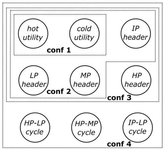
Figure 7.
Overview of the units defined for the various utility system configurations.
2.4. The Overall Optimization Problem for Calculating the Refinery Energy Targets
By combining the above alternatives for process-to-process aggregation and utility system configurations, 25 different cases were obtained. Under the condition of full site direct heat integration (case g), there is no need for the steam network for indirect heat transfer and the excess heat is released at too low temperature levels for generating steam for power production applications. There is therefore no need to make further distinction between different utility system configurations in case g.
In addition, for each case, four values of minimum allowable temperature difference for heat exchanging (ΔTmin) were investigated: 0, 10, 20 and 30 °C. The case of zero temperature difference is only of theoretical interest since it would require infinite heat exchange surface area. This does not represent a technically feasible condition but provides the theoretical reference for maximum level of heat recovery. In case a-1, no direct process heat integration is allowed and no steam utility system is considered, which makes the choice of ΔTmin irrelevant.
Overall, 97 optimization problems were solved using the calculation framework. In each case, the input data were changed concerning the type and number of utility units, the definition of the neighbours of each process unit and the value of ΔTmin. The definition of neighbours for process units vary according to the different process-to-process aggregations (case a-g). Utility units can, however, exchange heat with all the other units and, furthermore, their size is variable and subject to optimization. The heat contributions of the utility units are consequently treated as optimization decision variables. The developed calculation framework automatically generates all the necessary equations thus considerably reducing the amount of time spent on problem formulation for each case. In general terms, the constraints describe heat transfer feasibility and mass continuity as linear inequalities and equalities.
The objective of maximum energy recovery was pursued in this analysis. The minimization of hot utility was achieved by optimizing the heat load distribution of process and utility units. The steam flows are in principle free to assume any size as long as they contribute to minimizing the hot utility demand. When steam is used only to transfer heat indirectly, the minimum amount of steam at each steam header that leads to minimizing the total hot utility requirement is estimated (i.e., the optimization calculation maximizes process direct heat integration). For the case in which turbines are also considered, the steam flows are instead maximized so as to maximize the power production while still guaranteeing the minimum hot utility demand.
The objective function was formulated as follows:
where:
- is the amount of hot utility, i.e., the heat released by fuel combustion in process furnaces and steam boilers
- , , , and represent the heat loads of steam generated at each steam header and that are used for process heating at the same header (i.e., do not include the steam that is expanded through turbines)
- is the total power generated by the turbines working between the HP and MP headers, between the HP and LP headers, and between the IP and LP headers
- The coefficients are weights of positive values
The weight coefficients were chosen to drive the optimization results towards solutions that achieve, in order of importance: minimum hot utility demand, minimum utilization of steam that does not contribute to power production, maximum power generation. The values of such coefficients should be chosen to ensure this priority order. Typically, it would be appropriate to set the weights according to the relative costs or economic values of the heat flows. In this work the following values were used: = 100; = 40; = 22; = 11; = 4; = 10.
The reader might observe that in principle hot utility could be used to generate extra steam used for power generation only, that is by increasing the hot utility, more power can be generated than what could be produced by recovering excess heat only. However, by using a sufficiently larger weight for the hot utility compared to that for power generation (where also energy conversion efficiency needs to be considered), this results in an increase in the objective function, and such a solution will therefore not be obtained from the optimization.
3. Results and Discussion
In Table 1 the calculated energy targets for all the cases are shown. The large number of system aggregation cases could be solved with only minor user efforts thanks to the automatic generation of model equations in the computational framework. The absolute minimum hot utility demand, case g with ΔTmin equal to 0 °C, is 116 MW which means that the current hot utility (434 MW) can be reduced by maximum 73%.

Table 1.
Calculated minimum hot utility (MW) for the different process-to-process and process-to-utility aggregation levels considered and difference compared to the current hot utility demand (434 MW) within brackets. (* For utility configuration 4 cogeneration targets (MW) are also shown: hot utility/power).
Furthermore, the results show that by allowing complete heat integration within each area and by transferring heat to adjacent areas (case f) the same MER target can be obtained as for case g (complete site heat integration). Note also that in cases f and g, independently of the value of ΔTmin, there is no excess heat available above 220 °C (saturation temperature of the IP steam) and therefore no power can be generated with the considered steam turbine layout.
The targets closest to the current hot utility demand are obtained for case b-1 (complete process-to-process integration within units and no steam network) and a ΔTmin of 20 or 30 °C. However, this system aggregation level does not represent the current refinery heat integration very well. In reality, the refinery uses the steam network quite extensively for heat integration between units. On the other hand, the targeted process-to-process heat exchange within units is not fully achieved.
In the following sections, the results from Table 1 are further discussed with the help of diagrams.
3.1. The Extreme Cases of No Direct Heat Recovery (Case a) and of Unrestricted Heat Recovery across the Complete Site (Case g)
The cases in which no direct heat integration is allowed between process streams (cases a-2 to a-4) provide indications about possible levels of hot utility that can be achieved by indirect heat exchange only. This corresponds to completely avoiding direct heat exchange between process streams, including existing heat exchangers within process plants such as feed-effluent heat exchangers around reactors. Avoiding direct heat exchange potentially has considerable advantages for process operability, safety and degree of freedom in refinery layout. On the other hand, a large amount of steam needs to be transported within and between process units to minimize the refinery energy demand which may require large investments in piping, coolers and heaters. The energy targets of cases a-2 to a-4 and case g are shown in Figure 8 for different values of ΔTmin.
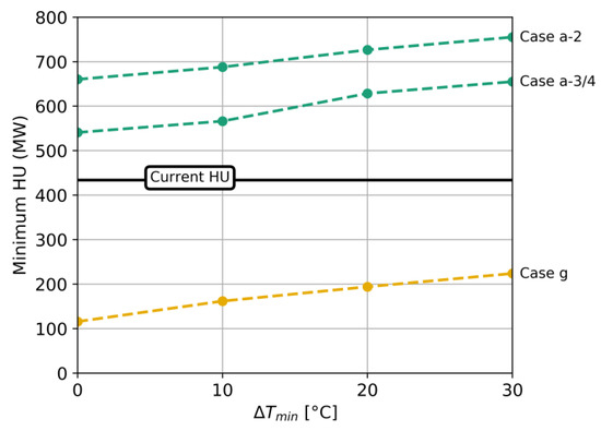
Figure 8.
Hot utility targets for cases without direct heat recovery (cases a-2 to a-4) and with unrestricted heat recovery across the complete site (case g).
Case g provides a theoretical MER reference that can be used to estimate the energy penalty associated with the restrictions introduced in the other, more relevant cases discussed hereafter. The figure shows that direct process heat recovery is of significant importance for the refinery energy efficiency. Compared to the current hot utility demand, the heat savings that can be achieved, theoretically, by further improvements in heat recovery is ranges from 52% to 73%, depending on the accepted values of ΔTmin.
Case a-2 is based on a steam network with steam cooling and heating at IP, MP and LP levels whereas cases a-3 and a-4 allow steam cooling and heating at HP level, which is currently not adopted at the refinery. This latter option can lead to a maximum 100 MW of additional heat savings.
3.2. The Role of Increasing Process-to-Process Aggregation
In practice, a combination of direct and indirect heat exchange is adopted to achieve heat recovery in large process sites. To estimate the contributions of these two different measures for the refinery case study, we first consider the recovery potential by direct heat transfer only (i.e., without the aid of the site wide steam network). The effect of process-to-process aggregation is shown in Figure 9 where case a-3 (no direct recovery, but only indirect heat exchange through the steam network) is shown for comparison.
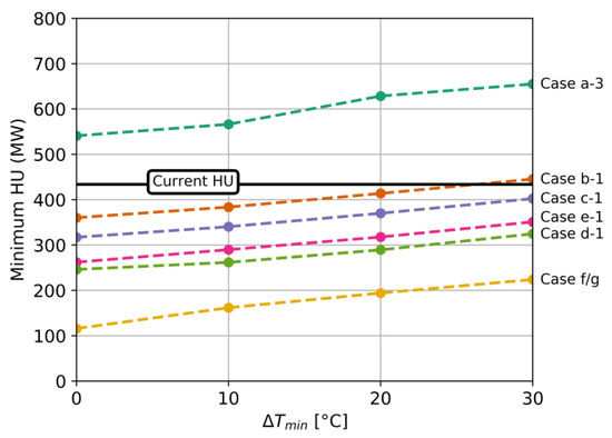
Figure 9.
Hot utility targets for cases with different levels of process-to-process aggregation without indirect heat exchange through steam network (case a-3 without direct heat integration but with steam network is also shown for comparison).
Interestingly, in case b-1, in which direct heat recovery is allowed to occur only within each unit and no steam system is considered, the hot utility target is similar to the current refinery heat demand. This corresponds to a scenario in which no site-wide steam network is used, and unit-dedicated furnaces and boilers are used to cover the hot utility demands of each process unit. Note that the actual “system aggregation” at the refinery would be best represented by utility configuration 4 (steam network with turbines) and process-to-process heat exchange allowed within units but without all possibilities exhausted (i.e., a case somewhere between case a-4 and b-4).
By allowing heat to be exchanged directly between streams located in different but adjacent units, the hot utility demand can be further decreased by about 120 MW (difference in hot utility targets between case d-1 and case b-1). In particular, about 35 MW could be achieved by allowing cross unit recovery within the same area (case c-1) and another 85 MW could be achieved by allowing cross unit recovery to occur between units belonging to different but adjacent areas (case d-1). Alternatively, a similar reduction can be obtained if complete direct heat recovery is achieved within each area (case e-1).
Consequently, by assuming more realistic process-to-process aggregation levels, the heat savings potential is about 25% to 45% compared to the current hot utility demand. This corresponds to about half of the theoretical heat savings potential. However, this was estimated without considering the possible option of indirect heat transfer through the utility system. In the next section, the role of the steam network in increasing the site integration is discussed.
3.3. The Role of Process-to-Utility Aggregation
Figure 10 shows the hot utility targets calculated including the possibility of indirect heat exchange through the steam network. The advantage of exchanging heat indirectly through the steam network is clear for case b where direct heat recovery is allowed within each unit only. In this case, up to 130 MW of additional savings can be achieved with a site wide steam network (see difference between cases b-3 and b-1). The advantage is also clear for case e (when complete direct heat exchange is achieved within each area) where a steam network allows about 80 MW of additional heat savings (difference between e-3 and e-1, see Table 1).
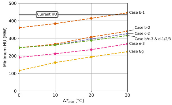
Figure 10.
Hot utility targets for the cases where a steam network is used to exchange heat indirectly in addition to different degrees of direct heat integration.
Conversely, no significant improvement of heat recovery is obtained by allowing indirect heat exchange through the steam network when direct heat exchange is allowed between adjacent units in case c and case d (compare e.g., the MER targets of cases d-1 and d-3). For case d, it can therefore be concluded that heat integration opportunities can be fully achieved by direct heat exchange only.
3.4. Cogeneration Targets
Figure 11 shows the power generation targets that can be achieved by expanding steam generated by process heat recovery for the different process-to-process aggregation cases.
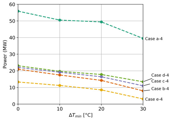
Figure 11.
Cogeneration targets for the different cases and different values of ΔTmin.
Generally, by increasing heat recovery, less excess heat is left for power generation, as can be observed by comparing cases a-4 and b-4. When no direct process heat exchange is allowed and heat recovery is achieved through the steam network only (case a-4), the amount of excess heat is large and about 40 to 55 MW power can be generated, depending on the value of ΔTmin allowed in coolers and heaters. Conversely, when direct heat exchange is allowed within each unit (case b-4) or each area (case e-4), much less excess heat can be recovered for power generation.
The effect of process integration on cogeneration targets is in reality more complex and does not involve only the amount of excess heat but also the temperature levels of the heat sources and sinks. This aspect can be seen by comparing the results of case b-4 with cases c-4 and d-4. Cases c and d allow direct heat exchange between adjacent units, thus introducing more degrees of freedom for direct heat integration. To the extent that more options of direct heat integration (cases c and d) will decrease the overall hot utility demand and reduce the required steam network capacity (i.e., compared to case b), it is expected that the power generation will also be decreased, if the excess waste heat is in appropriate temperature levels. However, cases b, c, and d achieve almost the same hot utility demand in the refinery case study (Table 1). When this happens, cases c and d allow for searching among more direct heat integration options (i.e., for the same minimum hot utility demand) to also maximise the power generation. This in turn allows to find which case of direct heat integration between process streams which best matches the steam network conditions so that more power can be generated.
3.5. Selection of Appropriate Refinery Energy Targets
It is reasonable to believe that direct heat exchange between units can lead to larger energy savings, but also to higher costs and more operability issues compared to indirect heat exchange through the steam network. To select appropriate energy targets, a first step should be to evaluate different cases of system aggregations, to get indications of the potential savings from allowing direct heat exchange within successively larger groups of process streams.
It should be noted that similar studies typically consider a combination of direct heat exchange within subsystems and indirect heat recovery via heat transfer for site-wide energy recovery, but only for one specified system aggregation level. The modelling approaches reported by Becker and Maréchal [33] or Bagajewics and Rodera [22] could, for example, correspond to either case b-2 or e-2, while the aggregation level corresponding to our case a-2/3 corresponds to a traditional grey-box TSHI approach. No previous studies have been found to report on the influence of different system aggregation levels. The case study presented in this paper demonstrates the advantage of our proposed approach, which is the systematic investigation of various system boundaries and levels of heat exchange restrictions. Such results can be used to decide for the right level of aggregation before more detailed targeting and design studies.
The results presented above for the case study refinery indicate that from a hot utility standpoint there is no actual benefit in implementing direct heat exchange between adjacent units (case c and d) since similar targets can be achieved by indirect heat exchange through the steam network (case b-3). In fact, the increase in power generation for case d-4 compared to case b-4 is small and unlikely to justify the additional costs of direct heat exchange between plant areas.
Figure 10 also shows that by accepting a ΔTmin of 10 °C in case b-3 (direct heat exchange only within the same unit, plus steam network for indirect heat recovery) a similar hot utility target is obtained as for case e-3 (direct heat exchange within units and between all units in the same process area, plus steam network) with a ΔTmin of 30 °C. While the first case with a lower ΔTmin likely leads to larger heat exchanger areas and associated capital costs, the latter case is likely to lead to higher piping costs as well as being associated with more challenges related to operability.
Overall, cases b-3 and b-4 correspond to more realistic conditions for establishing appropriate levels for refinery MER targets. In these cases, the theoretical energy savings compared to the current hot utility usage are in the range between 115 and 175 MW, depending on the accepted levels of ΔTmin, which corresponds to a potential reduction of 26 to 40% of the hot utility demand.
In cases b-3 and b-4, no heat exchange is allowed between process units. This means that all streams in a process unit belong entirely to the same subsystem and heat cascade. Consequently, there is no need to optimize how the heat load of process streams should be distributed over different heat cascades. Accordingly, only steam distribution is optimized. In case b-3, the steam distribution is optimized for minimum hot utility and, in case b-4, also for maximum cogeneration. The calculated optimal amounts of steam at different pressure levels that is used or produced in the various units is shown for case b-3 in Table 2 and for case b-4 in Table 3, for a ΔTmin of 10 °C.
Table 2.
Possible optimal distribution of steam consumption and production in different refinery units for the case in which direct heat exchange is allowed within process units only and a site-wide steam network configuration without turbines is considered (case b-3, ΔTmin = 10 °C). Below, cond = condensation, i.e., steam consumption and evap = evaporation, i.e., steam production.
Table 3.
Possible optimal steam distribution and production in different refinery units for the case in which direct process heat integration is allowed within units only and a site wide steam network with turbines is used (case b-4, ΔTmin = 10 °C, power generation = 17.5 MW). Below, cond = condensation, i.e., steam consumption and preh = preheating, evap = evaporation, spht = superheating, i.e., preh+evap+spht refers to steam production.
As already discussed above, there are multiple possible optimal solutions since the amount of excess heat is large and therefore steam can be produced in different units. For example, the solution shown in Table 2 does not consider the rather common solution of producing steam in the FCC unit.
As shown in Table 3, in case b-4 steam is also raised and used for power generation. In particular, this solution shows that large amounts of excess heat can be recovered from the vacuum distillation unit (VDU) and from the fluid catalytic cracking unit (FCC). About 17.5 MW of power can be generated, of which 16.2 MW are generated in the HP-LP turbines and 1.2 MW are generated in the IP-LP turbines. Overall, the net excess heat amounts to 51.8 MW and 75 MW is the heat recovered at high temperature level and delivered at lower temperature levels by steam expansion.
5. Conclusions
In this work, various energy recovery targets for a complex oil refinery were quantified, representing different degrees of limitations for direct process heat exchange and different options for steam utility system integration. As demonstrated in the case study, the proposed approach allows for evaluating a large number of system integration cases with only minor modelling efforts. The scenarios analysed range from allowing direct process heat exchange across the entire site to requiring that any heat recovery must be achieved through the steam utility system. More realistic scenarios include a combination of direct process heat exchange within and between neighbouring process units and heat recovery via the steam utility system for site-wide heat integration.
The theoretical potential savings at the refinery, quantified by comparing the current hot utility demand (434 MW) and the site global targets (between 116 MW and 224 MW for ΔTmin ranging between 0 and 30 °C), are about 48% to 73% depending, on the accepted minimum temperature difference for heat exchange (ΔTmin). By taking into account different levels of practical heat exchange limitations based on layout and operability principles, the estimated hot utility targets are instead between 246 and 316 MW for ΔTmin varying between 0 and 30 °C, which corresponds to potential savings between 27% to a theoretical maximum of 43%. Reasonably achievable values of ΔTmin of 10–20 °C, suggest around 35% as maximum level of such savings.
The results indicate that for the studied refinery, direct process heat exchange should be mainly pursued within process unit, since additional heat recovery at the site can be more easily achieved by indirect heat exchange through the site-wide steam network, which enables more flexible and reliable process operation.
By examining in more detail the temperature intervals around those corresponding to the steam headers we see that the theoretical amounts of excess heat available in some units such as the vacuum distillation unit or the visbreaker unit and the FCC are significant and sufficient to cover the heat demands of other units by means of a site wide steam network. If only the process heating demand is considered, this means that direct heat exchange is only partially necessary in those units where heat demand appears at temperature levels compatible with LP or MP steam, since the steam that can be generated in other units is abundant. This shows on the other hand that high-temperature excess heat from single process units can be used to generate steam which in turn can be used to generate power. The analysis suggests that up to about 17 MW can be generated by only recovering process excess heat (i.e., without further steam generation in dedicated boilers).
Overall the analysis of the refinery illustrated that direct and indirect heat exchange are necessarily intertwined. The proposed systematic assessment of different process-to-process aggregations for which direct process heat exchange is allowed in combination with capacity sizing of steam utility systems presents a new approach to complex energy targeting analysis. The novel approach allows for highlighting the most critical opportunities for increasing energy savings in a complex multi-plant process site, while enabling consideration of practical limitations to heat integration.
This study focused on energy targeting for increased heat recovery in the current process site. Further research could, for example, aim at a more explicit consideration of costs, suggest systematic procedures for identifying heat exchange restrictions, or look into how the proposed approach could be used to consider constraints for heat integration when integrating new processes in existing sites.
Author Contributions
Conceptualization, E.S. and M.M.; formal analysis, E.S. and M.M.; investigation, E.S. and M.M.; methodology, M.M.; software, M.M.; supervision, S.H. and S.P.; validation, E.S., S.H. and S.P.; visualization, E.S. and M.M.; writing—original draft, E.S.; writing—review and editing, S.H. and S.P. All authors have read and agreed to the published version of the manuscript.
Funding
This research was funded by Chalmers Energy Area of Advance and other internal faculty funding.
Acknowledgments
Anders Åsblad and Eva Andersson at CIT Industriell Energi are gratefully acknowledged for their inputs regarding the refinery processes and utility system.
Conflicts of Interest
The authors declare no conflict of interest.
Nomenclature
| Abbreviations | |
| ARU | Amine Recovery Unit |
| Cond | Condensation |
| CDU | Crude Distillation Unit |
| CRU | Catalytic Cracking Reforming Unit |
| CU | Cold Utility |
| Evap | Evaporation |
| FCC | Fluid Catalytic Cracker unit |
| HEN | Heat Exchanger Network |
| HP | High-Pressure steam |
| HPU | Hydrogen Production Unit |
| HU | Hot Utility |
| ICR | Hydrocracking unit |
| IP | Intermediate-Pressure steam |
| ISO | Isomerization unit |
| LP | Low-Pressure steam |
| MER | Minimum Energy Requirement |
| MEROX | Mercaptan Oxidation unit |
| MHC | Mild Hydro Cracker unit |
| MP | Medium-Pressure steam |
| NHTU | Naphtha HydroTreating Unit |
| POLY | Polymerization unit |
| Preh | Preheating |
| Spht | Superheating |
| SRU | Sulphur Recovery Unit |
| SS | SynSat unit |
| TGTU | Tall Gas Treatment Unit |
| TSA | Total Site Analysis |
| TSHI | Total Site Heat Integration |
| VBU | VisBreaker Unit |
| VDU | Vacuum Distillation Unit |
| Symbols used in main manuscript | |
| objective function | |
| amount of hot utility | |
| heat load of steam generated at steam header (=LP, MP, IP or HP) and used for process heating at the same header | |
| total power generated by the turbines | |
| coefficients for weighting the terms of the objective function | |
| Symbols used in Appendix | |
| matrix with all heat excess coefficients | |
| vector with all constant heat contributions of local units of fixed size | |
| , size of a variable-size pivot unit | |
| local unit of fixed size | |
| local unit of variable size | |
| lower bound for the size of a local unit of variable size | |
| lower bound for the size of a pivot unit of variable size | |
| pivot unit of fixed size | |
| pivot unit of variable size | |
| heat load of stream at temperature interval | |
| sum of the heat excess of all local units of fixed size at temperature interval | |
| heat excess cascaded from the temperature interval immediately above | |
| heat excess of local unit of variable size at temperature interval | |
| heat excess of stream s of pivot unit of fixed size at temperature interval | |
| heat excess of stream t of pivot unit of variable size at temperature interval | |
| , array of all heat cascade coefficients | |
| temperature interval | |
| upper bound for the size of a local unit of variable size | |
| upper bound for the size of a pivot unit of variable size | |
| unit size multiplication factor for local units of variable size | |
| stream split variable for steam of a pivot unit of fixed size | |
| stream split variable for stream of a pivot unit of variable size | |
| , array of all decision variables for heat cascade | |
| heat cascade/maximal clique | |
Appendix A. A Graph Theory Approach to Organize Complex Patterns of Heat Exchange Limitations
Appendix A.1. Representing Heat Exchange Limitations in Heat Integration Graphs
Process units can be represented as nodes in a graph where edges connecting units represent heat integration opportunities (Figure A1). A unit is defined as neighbour of another unit when it can exchange heat directly with that unit. A missing edge between two units indicate a heat exchange limitation (see Figure 4, Figure 5 and Figure 6 in the main manuscript for examples of heat integration graphs from the studied refinery).

Figure A1.
Examples of graph representation of heat integration opportunities between system stream subsets: (a) no heat exchange restrictions; (b) with heat exchange restrictions and total site stream subset; (c) with partial restrictions; (d) with partial restrictions and with total site stream subset.

Figure A1a represents the fully integrated case where all the units are connected together. A Pinch Analysis cascade can be calculated for the whole process stream set. Similarly, a trivial graph where all the units are disconnected from the others can be also defined. In this case the MER target can be calculated by computing one cascade for each unit.
Figure A1b shows the case in which one unit, in this case unit 5, can be heat integrated with all the other units and therefore can be used to transfer heat indirectly from one unit to another. This is for instance the case usually considered by Total Site Analysis in which a common utility system such as a steam network is used for exchanging heat between different process zones.
In Figure A1c a heat exchange limitation exists between each unit and one of the other 3 units, e.g., direct heat exchange is not possible between unit 2 and unit 3 and between unit 1 and unit 4.
In Figure A1d, unit 5 can exchange heat with all the other units and is therefore used to achieve intermediate heat transfer between all the units, but some degree of direct heat exchange is also allowed between the other units. In fact, it is quite common that in a process heat integration occurs between process units directly and to some degree also through a site wide heat collection and distribution system (unit 5 in Figure A1d).
Appendix A.2. Identifying Maximal Cliques in Heat Integration Graphs
Based on the edges in the graphs, it is possible to identify subsystems, in graph theory called maximal subgraphs or maximal cliques, here represented with the symbol ψ.
A subgraph or clique is a portion of a graph which nodes are completely connected with each other. A clique is called maximal if no node of the graph outside the clique is adjacent to all the members of the clique. If the graph is connected, that is if a path that passes through all the units exists, and if the graph is not completely connected, it follows necessarily that two or more maximal cliques share one or more nodes (units). It is therefore useful to define two types of units:
- local units: units that participate to only one maximal clique
- pivot units: units that participate to more than one maximal clique
The thermal streams of a local unit participate completely to the maximal clique cascade, while the streams of a pivot unit may participate to more than one cascade (see also shaded circles/boxes in the heat integration graphs in Figure 4, Figure 5 and Figure 6, Section 2.3.1). Depending on the way in which such streams are distributed to contribute to one clique or another, different heat integration opportunities can be exploited and therefore different amounts of hot and cold utility are required to satisfy the whole system thermal balance. Different optimization strategies can be adopted to tackle the problem of finding the optimal heat distribution of streams belonging to pivot units. Here we show first the application of the clique approach for a few simple examples.
The following maximal cliques can be identified for the case in Figure A1b: ψ1 = {1,5}; ψ2 = {2,5}; ψ3 = {3,5}; ψ4 = {4,5}. The four cliques share unit 5, here shown in bold, which is the only pivot unit. Optimization in this case should involve only the streams belonging to this unit. This corresponds to traditional Total Site Analysis where for instance a steam network is designed to accomplish the integration between separate process plants (equivalent in our terminology with separate cliques).
In the example in Figure A1c, the following maximal cliques can be identified: ψ1 = {1,2}; ψ2 = {2,4}; ψ3 = {3,4}, ψ4 = {1,3}. Unlike the case in Figure 1b where a single pivot unit appears, all units are of the pivot type here. This means that the distribution of thermal streams in all units in different separate cliques shall be optimized.
This approach is made clearer when looking at the example in Figure A1d where the following maximal cliques are present: ψ1 = {1,3,5}; ψ2 = {1,2,5}; ψ3 = {2,4,5}; ψ4 = {3,4,5}. In this case all the 5 units are of pivot type but there are 4 thermal cascades to consider.
Figure A2 presents a more complex case with 8 units where only 5 cascades need to be considered corresponding to 5 maximal cliques: ψ1 = {1,5,3}; ψ2 = {1,5,2}; ψ3 = {2,4,5,8}; ψ4 = {4,8,7}; ψ5 = {6,7,8}.

Figure A2.
Example of complex problem of constrained heat integration and its corresponding clique matrix.
Figure A2.
Example of complex problem of constrained heat integration and its corresponding clique matrix.

In large industrial sites, such as refineries, pulp and paper mills, or petrochemical sites, the number of units can be quite large and it can be difficult in practice to identify really separate “areas of integrity” and define a priori the maximal thermal cliques. However, a process operator or engineer can easily highlight the possible limitations to process integration between two streams or units. In our approach, the user (e.g., the process engineer) suggests the units and all the heat integration limitations (i.e., the edges to be removed in the heat integration graph). The thermal cliques can then be derived by automated procedures such as the algorithm by Bron and Kerbosch [36]. In our calculation framework this algorithm is applied to calculate the maximal cliques starting from the adjacency matrix of the heat integration graph which is built by recording for each unit the corresponding neighbours, that is, the units with which heat can be exchanged directly.
Appendix A.3. Translating Graph Theory Insights into Heat Transfer Feasibility Constraints
As previously introduced, graph theory insights can be used to identify relevant subsystems and simplify the formulation of heat transfer feasibility constraints in energy targeting analysis [37]. By distinguishing units from maximal cliques (i.e., thermal cascades), constrained energy targeting analysis can be organized as an optimization problem where a set of decision variables is associated to each pivot unit to control how different pivot streams should be distributed into different maximal cliques. The heat transfer feasibility can then be ensured by a set of inequality constraints for separate clique cascades. Ultimately, these sets of constraints are considered simultaneously for the whole system, thereby avoiding iterative or recursive procedure.
When determining the optimal contribution of a given unit or stream in a given temperature interval, the heat transfer feasibility condition is imposed at each temperature interval as an inequality constraint as shown in Equation (A1):
where is the heat load of stream h (positive if hot stream, negative if cold stream) at temperature interval , and is the heat excess cascaded from the temperature interval immediately above. Accordingly, the Pinch Point is the condition in which the cumulative heat load at a given temperature interval is equal to 0.
To rewrite Equation (A1) for the thermal cascade of a maximal clique, we introduce a notation to distinguish between local and pivot units. In addition, we make a distinction between utility units, which size is not known and has to be optimized, and process units with fixed sizes. For the different types of units, different heat contributions should be considered in the clique heat cascade:
- Local unit of fixed size: The sum of the heat contributions of its h streams appears as a fixed value in the interval heat balance of the corresponding clique
- Local unit of variable size: the sum of the heat contributions of its i streams multiplied by a unit size multiplication factor appears as a variable in the interval heat balance of the corresponding clique
- Pivot unit of fixed size: Heat contributions of its s streams each multiplied by a stream split variable appear as variables in the interval heat balances of two or more cliques
- Pivot unit of variable size: Heat contributions of its t streams each multiplied by a stream split variable appear as variables in the interval heat balances of two or more cliques
Equation (A1) can now be written for a clique cascade with the introduced notation as follows:
In principle the number and magnitude of temperature intervals in one clique thermal cascade can be different from those of another clique.
In our work we used one split variable or for each pivot stream and clique, i.e., the stream is forced to split in the same way along all the temperature intervals. In principle, the pivot stream splits could be temperature interval specific, so that a different set of such variables was defined for each pivot stream and each temperature interval. In some situations, this could allow for identifying solutions with better energy targets. In large problems, however, this causes the number of variables to explode very quickly and simplification is necessary to reduce problem complexity.
In Equation (A2), , the heat excess at a temperature interval , is dependent on , the heat excess of the temperature above. Equation (A2) can be rewritten by explicitly substituting as follows:
Using a simpler notation, Equation (A3) can be rewritten as:
where in each heat cascade, :
- is the heat excess of local unit of variable size at temperature interval
- is the heat excess of stream s of pivot unit of fixed size at temperature interval
- is the heat excess of stream t of pivot unit of variable size at temperature interval
- is the sum of the heat excess of all local units of fixed size at temperature interval
By further grouping all the cascade coefficients in one array , and the decision variables in one array , Equation (A4) can be written in condensed form as follows:
Equation (A5) can be written for all the temperature intervals leading to the final complete form of the heat transfer feasibility constraint in a general maximal clique :
This can be further symbolically simplified into where is the matrix containing all the heat excess coefficients , with as many rows as the number of temperature intervals and as many column as the number of decision variables . This variable vector includes all the size variables for local units , the split variables for streams of pivot units of fixed size , and the split variables for streams of pivot units of variable size . The vector has as many components as the number of temperature intervals and includes all the constant heat contributions of local units of fixed size.
Appendix A.4. Mass Continuity Equations and Bounds
For a pivot unit of fixed size each stream can be split in as many parts as the number of maximal cliques it belongs to and the sum of the split fractions should add to unity:
For a pivot unit of variable size, such mass balance may also vary with the size of the pivot unit. Accordingly, the sum of the split fractions should lie between the lower and upper bounds of pivot unit size, here indicated with and , respectively:
Equation (A8) also ensures that all streams of a variable size unit (such as a utility system) are scaled equally.
Finally, a set of equations is necessary for imposing the upper and lower bounds of the local units of variable size:
Appendix A.5. Linearized models of Utility Units based on Energy Conversion Technologies
To be able to retain the linearity of the optimization model, linear models of utility systems were developed. A typical problem that we want to address is that of establishing the optimal values of the various network mass flow rates to simultaneously minimize hot utility demand and maximize power production (co-generation targets).
When dealing with units of variable size that may feature variable degree of mixing of material streams with different enthalpy content, some simplification must be introduced in order to describe the relations between mass and energy balances through linear expressions. This is for instance the case of the steam network layout, which is shown with some simplification in Figure A3.

Figure A3.
Example of simple steam network used in large process industrial sites.
Figure A3.
Example of simple steam network used in large process industrial sites.

A typical non-linearity of thermodynamic systems occurs when two or more streams with different thermodynamic states are mixed. To avoid this, the steam states can be kept close to saturation conditions with the help of desuperheaters or flash drums so that the state of different steam lines that are going to be mixed and that resulting from mixing are the same. By assuming that this is the case a modelling approach based on superimposition of elementary steam cycles can be applied (see also [38]).
Elementary cycles are defined in such a way that no splitting or mixing is present, as shown in Figure A4. In addition to steam turbine cycles, it is often relevant to also include an elementary cycle representing the optional feature of steam raising and steam condensation at the same pressure level (right side of Figure A4). In order to decompose the whole steam network into elementary cycles, parts of the steam network that are shared between the cycles must be defined to have equal thermodynamic states. This way mixing can be described by simple mass continuity constraints. In practice, these shared portions of the network usually correspond to common steam pressure levels. This approach allows to dramatically simplify the equations to be used for describing steam systems in our optimization framework without causing the energy and mass balances to depart too much from reality. With this approach, mass balances at mixing or splitting points in steam headers are implicitly imposed by Equation (A8). Each cycle is treated as a unit, which necessarily is of pivot type and variable size and therefore participates to more than one clique and their size decided upon optimization.

Figure A4.
Elementary cycles considered to model the steam network in Figure A3.
Figure A4.
Elementary cycles considered to model the steam network in Figure A3.

References
- Smith, R. Chemical Process: Design and Integration, 2nd ed.; John Wiley and Sons: Chichester, UK, 2016; 920p. [Google Scholar]
- Klemeš, J.J.; Varbanov, P.S.; Walmsley, T.G.; Jia, X. New directions in the implementation of Pinch Methodology (PM). Renew. Sustain. Energy Rev. 2018, 98, 439–468. [Google Scholar] [CrossRef]
- Salazar, J.M.; Diwekar, U.M.; Zitney, S.E. Rigorous-simulation pinch-technology refined approach for process synthesis of the water-gas shift reaction system in an IGCC process with carbon capture. Comput. Chem. Eng. 2011, 35, 1863–1875. [Google Scholar] [CrossRef]
- Telang, K.S.; Chen, X.; Pike, R.W.; Knopf, F.C.; Hopper, J.R.; Saleh, J.; Yaws, C.L.; Waghchoure, S.; Hedge, S.C.; Hertwig, T.A. An advanced process analysis system for improving chemical and refinery processes. Comput. Chem. Eng. 1999, 23, S727–S730. [Google Scholar] [CrossRef]
- Chew, K.H.; Klemeš, J.J.; Alwi, S.R.W.; Abdul Manan, Z. Industrial implementation issues of total site heat integration. Appl. Therm. Eng. 2013, 61, 17–25. [Google Scholar] [CrossRef]
- Svensson, E.; Eriksson, K.; Wik, T. Reasons to apply operability analysis in the design of integrated biorefineries. Biofuels, Bioprod. Biorefining 2015, 9, 147–157. [Google Scholar] [CrossRef]
- Marton, S.; Harvey, S.; Svensson, E. Investigating operability issues of heat integration for implementation in the oil refining industry. In Proceedings of the ECEEE Industrial Summer Study, Berlin, Germany, 12–14 September 2016; pp. 495–503. [Google Scholar]
- Al-Riyami, B.A.; Klemeš, J.; Perry, S. Heat integration retrofit analysis of a heat exchanger network of a fluid catalytic cracking plant. Appl. Therm. Eng. 2001, 21, 1449–1487. [Google Scholar] [CrossRef]
- Al-Mutairi, E.M. Optimal Design of Heat Exchanger Network in Oil Refineries. Chem. Eng. Trans. 2010, 21, 955–960. [Google Scholar]
- Dinçer, S.; Şentarli, İ. Heat-integration retrofit study of a petroleum refinery. Appl. Energy 1991, 38, 253–262. [Google Scholar] [CrossRef]
- Ji, S.; Bagajewicz, M. Design of crude fractionation units with preflashing or prefractionation: Energy targeting. Ind. Eng. Chem. Res. 2002, 41, 3003–3011. [Google Scholar] [CrossRef]
- Yimyam, B.; Siemanond, K. Retrofit with Exchanger Relocation of Crude Preheat Train under Different Kinds of Crude Oils. Chem. Eng. Sci. 2012, 29, 319–324. [Google Scholar]
- Cui, C.; Sun, J. Coupling design of interunit heat integration in an industrial crude distillation plant using pinch analysis. Appl. Therm. Eng. 2017, 117, 145–154. [Google Scholar] [CrossRef]
- Goodarzvand-Chegini, F.; Farkhondehkavaki, M.; Gougol, M. Application of heat integration in hydrocracking process. Asia-Pac. J. Chem. Eng. 2011, 6, 886–895. [Google Scholar] [CrossRef]
- Walmsley, T.G.; Lal, N.S.; Varbanov, P.S.; Klemeš, J.J. Automated retrofit targeting of heat exchanger networks. Front. Chem. Sci. Eng. 2018, 12, 630–642. [Google Scholar] [CrossRef]
- Dhole, V.R.; Linnhoff, B. Total site targets for fuel, co-generation, emissions, and cooling. Comput. Chem. Eng. 1993, 17, S101–S109. [Google Scholar] [CrossRef]
- Klemeš, J.; Dhole, V.R.; Raissi, K.; Perry, S.J.; Puigjaner, L. Targeting and design methodology for reduction of fuel, power and CO2 on total sites. Appl. Therm. Eng. 1997, 17, 993–1003. [Google Scholar] [CrossRef]
- Liew, P.Y.; Theo, W.L.; Wan Alwi, S.R.; Lim, J.S.; Abdul Manan, Z.; Klemeš, J.J.; Varbanov, P.S. Total Site Heat Integration planning and design for industrial, urban and renewable systems. Renew. Sustain. Energy Rev. 2017, 68, 964–985. [Google Scholar] [CrossRef]
- Jamaluddin, K.; Wan Alwi, S.R.; Abdul Manan, Z.; Hamzah, K.; Klemeš, J.J. A Process Integration Method for Total Site Cooling, Heating and Power Optimisation with Trigeneration Systems. Energies 2019, 12, 1030. [Google Scholar] [CrossRef]
- Tarighaleslami, A.H.; Walmsley, T.G.; Atkins, M.J.; Walmsley, M.R.W.; Liew, P.Y.; Neale, J.R. A Unified Total Site Heat Integration targeting method for isothermal and non-isothermal utilities. Energy 2017, 119, 10–25. [Google Scholar] [CrossRef]
- Rodera, H.; Bagajewicz, M.J. Targeting procedures for energy savings by heat integration across plants. AIChE J. 1999, 45, 1721–1742. [Google Scholar] [CrossRef]
- Bagajewicz, M.; Rodera, H. Multiple plant heat integration in a total site. AIChE J. 2002, 48, 2255–2270. [Google Scholar] [CrossRef]
- Bagajewicz, M.; Rodera, H. On the use of heat belts for energy integration across many plants in the total site. Can. J. Chem. Eng. 2001, 79, 633–642. [Google Scholar] [CrossRef]
- Bandyopadhyay, S.; Varghese, J.; Bansal, V. Targeting for cogeneration potential through total site integration. Appl. Therm. Eng. 2010, 30, 6–14. [Google Scholar] [CrossRef]
- Ghannadzadeh, A.; Perry, S.; Smith, R. Cogeneration targeting for site utility systems. Appl. Therm. Eng. 2012, 43, 60–66. [Google Scholar] [CrossRef]
- Ren, X.Y.; Jia, X.X.; Varbanov, P.S.; Klemeš, J.J.; Liu, Z.Y. Targeting the cogeneration potential for Total Site utility systems. J. Clean. Prod. 2018, 170, 625–635. [Google Scholar] [CrossRef]
- Stijepovic, M.Z.; Linke, P. Optimal waste heat recovery and reuse in industrial zones. Energy 2011, 36, 4019–4031. [Google Scholar]
- Chen, C.L.; Lin, C.Y.; Lee, J.Y. Retrofit of steam power plants in a petroleum refinery. Appl. Therm. Eng. 2013, 61, 7–16. [Google Scholar] [CrossRef]
- Chen, C.L.; Chen, H.C. A mathematical approach for retrofit and optimization of total site steam distribution networks. Process Saf. Environ. Prot. 2014, 92, 532–544. [Google Scholar] [CrossRef]
- Marton, S.; Svensson, E.; Subiaco, R.; Bengtsson, F.; Harvey, S. A steam utility network model for the evaluation of heat integration retrofits—A case study of an oil refinery. JSDEWES 2017, 5, 560–578. [Google Scholar] [CrossRef][Green Version]
- Zhang, B.; Wu, S.; Chen, Q. An optimization procedure for retrofitting process energy systems in refineries. Comput. Aided Chem. Eng. 2012, 31, 1005–1009. [Google Scholar]
- Wang, Y.; Chang, C.; Feng, X. A systematic framework for multi-plants Heat Integration combining Direct and Indirect Heat Integration methods. Energy 2015, 90, 56–67. [Google Scholar] [CrossRef]
- Becker, H.; Maréchal, F. Energy integration of industrial sites with heat exchange restrictions. Comput. Chem. Eng. 2012, 37, 104–118. [Google Scholar] [CrossRef]
- Maréchal, F.; Kalitventzeff, B. Restricted matches and minimum cost of energy requirements: tools and methodology for producing practical solutions. In Proceedings of the PRES—The 2nd Conference on Process Integration and Optimisation for Energy Saving and Pollution Reduction, Budapest, Hungary, 31 May–2 June 1999; pp. 433–438. [Google Scholar]
- Ahmad, S.; Hui, D.C.W. Heat recovery between areas of integrity. Comput. Chem. Eng. 1991, 15, 809–832. [Google Scholar] [CrossRef]
- Amidpour, M.; Polley, G.T. Application of problem decomposition in process integration. Chem. Eng. Res. Des. 1997, 75, 53–63. [Google Scholar] [CrossRef]
- Bron, C.; Kerbosch, J. Algorithm 457: Finding All Cliques of an Undirected Graph. Commun. ACM 1973, 16, 575–577. [Google Scholar] [CrossRef]
- Morandin, M. A generalized approach to handle heat exchange restrictions in energy targeting. Chem. Eng. Trans. 2013, 35, 157–162. [Google Scholar]
- Morandin, M.; Toffolo, A.; Lazzaretto, A. Superimposition of Elementary Thermodynamic Cycles and Separation of the Heat Transfer Section in Energy Systems Analysis. J. Energy Resour. Technol. 2013, 135, 021602-1–021602-10. [Google Scholar] [CrossRef]
- Preem, A.B. Preem’s Refineries Are the Best at Carbon Dioxide Emissions in Europe (in Swedish: Preems Raffinaderier är bäst på Koldioxidutsläpp i Europa). Press Release. Available online: https://www.preem.se/om-preem/press/nyhetsrum/ (accessed on 7 January 2020).
- Brau, J.-F. Production of Hydrogen for Oil Refining by Thermal Gasification of Biomass: Process Design, Integration and Evaluation. Licentiate Thesis, Chalmers University of Technology, Göteborg, Sweden, 22 November 2013. [Google Scholar]
- Brau, J.-F.; Morandin, M. Biomass-based hydrogen for oil refining: Integration and performances of two gasification concepts. Int. J. Hydrogen Energy 2014, 39, 2531–2542. [Google Scholar] [CrossRef]
- Andersson, V.; Franck, P.-Å.; Berntsson, T. Techno-economic analysis of excess heat driven post-combustion CCS at an oil refinery. Int. J. Greenh. Gas Control 2016, 45, 130–138. [Google Scholar] [CrossRef]
- Andersson, E.; Franck, P.-Å.; Åsblad, A.; Berntsson, T. Pinch Analysis at Preem LYR; Report; Chalmers University of Technology: Göteborg, Sweden, 2013; Available online: https://research.chalmers.se/publication/193621 (accessed on 28 August 2019).
- Åsblad, A.; Andersson, E.; Eriksson, K.; Franck, P.-Å.; Svensson, E.; Harvey, S. Pinch Analysis at Preem LYR II—Modifications; Report; Chalmers University of Technology: Göteborg, Sweden, 2014; Available online: https://research.chalmers.se/publication/198580 (accessed on 28 August 2019).
- Marton, S. Operability Considerations for Retrofit Design of Industrial Process Energy Systems. Licentiate Thesis, Chalmers University of Technology, Göteborg, Sweden, 28 November 2018. [Google Scholar]


© 2020 by the authors. Licensee MDPI, Basel, Switzerland. This article is an open access article distributed under the terms and conditions of the Creative Commons Attribution (CC BY) license (http://creativecommons.org/licenses/by/4.0/).