Abstract
Power generation from wind farms is traditionally modeled using power curves. These models are used for assessment of wind resources or for forecasting energy production from existing wind farms. However, prediction of power using power curves is not accurate since power curves are based on ideal uniform inflow wind, which do not apply to wind turbines installed in complex and heterogeneous terrains and in wind farms. Therefore, there is a need for new models that account for the effect of non-ideal operating conditions. In this work, we propose a model for effective axial induction factor of wind turbines that can be used for power prediction. The proposed model is tested and compared to traditional power curve for a 2.5 MW horizontal axis wind turbine. Data from supervisory control and data acquisition (SCADA) system along with wind speed measurements from a nacelle-mounted sonic anemometer and turbulence measurements from a nearby meteorological tower are used in the models. The results for a period of four months showed an improvement of 51% in power prediction accuracy, compared to the standard power curve.
1. Introduction
Renewable energies continue to grow and their contribution to the supply of electricity to the power grid is increasing. The benefits of renewable energy include reducing greenhouse gas emissions and air pollution, lowering cost and diversifying energy resources [1]. However, integration of renewable energy into the power grid while ensuring grid stability is challenging due to variability of power generation. The variability of wind power generation is due to variable wind speed, but also meteorological conditions such as turbulence, wind shear, wind veer and air density [2]. Therefore, accurate forecasting of wind power is crucial. The main applications of a wind energy forecast model include [3]:
- Wind resource assessment: at the initial stages of building a wind farm, the feasibility of the project is determined through estimating the amount of energy that can potentially be generated at the site.
- Wind farm control: power forecasting models can help wind farm operators optimize the power output of the plant.
- Managing supply and demand: ensuring grid stability is critical when integrating wind energy into the power grid, and accurate models for forecasting energy generation can help balancing authorities achieve this goal.
- Forecast of energy markets: renewable energy has made energy markets more dynamic, resulting in intra-day or rolling power markets which require accurate forecasts of energy production from wind farms in their transactions.
The standard power curve as typically used for the above applications, is a simple empirical model, provided by turbine manufacturers, that describes the relationship between ten-minute, hub-height, wind speed and wind turbine power. However, the accuracy of power prediction from only considering hub-height wind speed has been recently questioned. Clifton et al. [4] argue that not accounting for turbulence would result in 5–10% difference in actual power generation and manufacturer’s power curve predictions. Furthermore, the miss-alignment between the rotor and wind direction (yaw error), turbulence, density variation, wind shear, wind veer and thermal stability are among other variables whose effect on power generation has been investigated [5,6,7].
A novel approach to address the shortcomings of the standard power curves was introduced by Wagner et al. [5,8]. They investigated the effect of wind shear on wind turbine power generation and proposed using an equivalent wind speed instead of the hub-height wind speed in power curves. The proposed equivalent wind speed is the result of vertical integration of wind speed measurement at several heights to account for vertical variability of wind speed. This idea has been further developed to incorporate the effect of yaw error, density variation and turbulence intensity [2,6]. Furthermore, the effect of turbulence intensity [7,9,10,11] and atmospheric stability on wind turbine power generation has been studied [12,13]. Equivalent wind speed has also been implemented in regional scale models such as the Weather Research and Forecast (WRF) model [14].
A major weakness of current models implementing equivalent wind speed for modeling wind power is that they only consider the contribution of axial momentum flux for estimating power generation. This is because the current model only considers one-dimensional momentum theory. However, recent studies [15,16,17,18] show that vertical momentum fluxes also contribute to power generation of a wind turbine, and this contribution may be of the same order of magnitude as axial momentum fluxes under certain conditions. In this work, we start from two-dimensional formulation of momentum theory, and propose an induction curve model that forecasts wind energy generation based on data describing mean advection and turbulent fluxes of mean kinetic energy in the atmospheric boundary layer (ABL) in both horizontal and vertical directions. The proposed induction curve model shows promising results and can improve the accuracy of power prediction from a stand-alone wind turbine by 51%, compared to the standard models. However, as the results in [15,16,17,18] suggest, the contribution of vertical fluxes to power generation becomes more significant for wind turbines located in complex terrains or within a wind farm, and the induction curve model may provide improvement in power prediction for complex ABL flow conditions.
The paper is structured as follows: the process through which the induction curve model has been developed is laid out in Section 2, which entails implementation of an equivalent wind speed in combination with vertical momentum fluxes for modeling power generation. In Section 3 we present our dataset and describe the quality checks performed on the dataset, in order to prepare it for analysis. Finally, Section 4 and Section 5 summarize the results of the proposed model compared to the standard power curve and present concluding remarks.
2. Model Development
2.1. Standard Power Curve
Wind turbine manufacturers provide standard power curves for their turbines, following the guidelines established in the IEC 61400-12-1 standard [19]. Based on the actuator disk concept and one-dimensional momentum theory, the amount of power that a wind turbine can extract from the wind that passes through the rotor swept area is a function of kinetic energy flux into the rotor swept area and turbine efficiency as:
where is air density, A is the rotor swept area, U is wind speed and is the power coefficient. According to Betz [20], there is a limit to the amount of kinetic energy that wind turbines can extract, such that the power coefficient cannot exceed 0.593.
The standard wind turbine power curve is generated based on Equation (1). The power generated by the turbine and wind speed at the hub-height are averaged over ten-minute periods, to generate a relationship by fitting a curve to power output data as a function of hub-height wind speed. The turbine power output measurements come from SCADA data. However, obtaining measurements of wind speed at the inflow is more challenging. Typically, inflow wind speed is measured by tall meteorological towers, or it can be approximated using nacelle-mounted anemometers. However, the problem with measuring wind speed at the nacelle of the turbine is that it does not accurately represent wind conditions at the inflow and needs to be corrected. Therefore, a nacelle transfer function (NTF) is needed to correct wind speed measurements at the nacelle [21], which itself is specific to the wind turbine and site of measurement.
Alternatively, a number of studies have investigated the implementation of ground-based Doppler light detection and ranging systems (LIDARs) for characterization of wind turbine inflow conditions [22,23,24], whereas a more recent approach is to place the LIDARs on the wind turbine itself, in order to measure the incoming wind speed more accurately while the wake of the turbine can also be characterized [25,26,27]. A promising new approach to address this issue is using large-scale particle image velocimetry (PIV) to measure velocity profiles at the inflow and the wake of the turbine [28,29], which is still in development.
Once the inflow of the wind turbine is characterized and a power curve is generated, the resulting power curve can then be used for predicting power generation from the turbine. An example wind turbine power curves is shown in Figure 1, which consists of three main regions: cut-in region (I), operational region (II) and rated region (III). In this study we focus on the operational region of the power curve and wind speeds less than 11 m s−1. More information about power curves and how they are generated can be found in [19,21,30].
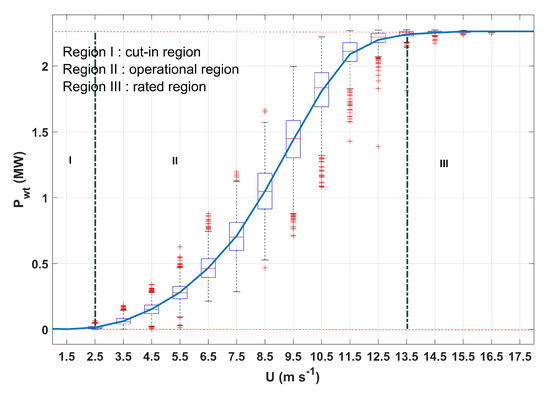
Figure 1.
A power curve derived for the 2.5 MW study turbine, using ten-minute data during the period of study, spanning from 20 February to 18 June 2018 and bins of 1 m s−1. Cut-in region (I), operational region (II) and rated region (III) are also shown.
2.2. Power Surface
Vahidzadeh et al. [2] proposed using a power surface instead of a power curve for modeling wind turbine energy generation. Power surface entails a two-dimensional bin-averaging method which considers the rotor equivalent wind speed and density as two independent variables. The available ten-minute data is divided into two-dimensional bins, and the power output is averaged over each bin. Then a surface is fitted to the bin-averaged data where . The rotor equivalent wind speed takes into account the effect of wind shear, wind veer, turbulence intensity, and yaw error, while considering air density as the second independent variable takes into account the effect of density variations. Figure 2 shows the two-dimensional bin-averaging method and the power surface that is fitted to the bin-averaged power data. The results from this model showed a 38% improvement in power prediction compared to the standard power curves. The inclusion of additional atmospheric variables in the power surface model significantly improves upon the standard power curve, but similar to the standard power curve it only considers momentum fluxes in the axial direction. Some recent studies have highlighted the importance of momentum fluxes in other directions [15,16,17] for power generation which signifies the need for adding non-axial momentum fluxes to power prediction models. In the next section, such a model is introduced. More information about the power surface model and details of its derivation can be found in [2].
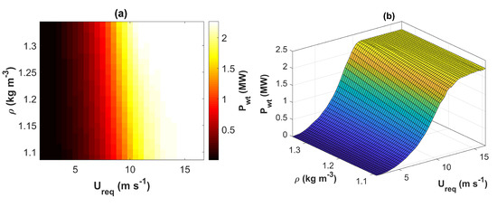
Figure 2.
(a) Two-dimensional binning of wind power in terms of rotor equivalent wind speed and density and (b) the resulting power surface.
2.3. Axial Flow Induction Factor Curve
The standard power curve presented in Section 2.1, describes wind turbine power generation only in terms of mean wind speed upstream of the wind turbine, and the power surface described in Section 2.2 only considers axial momentum fluxes. However, recent large eddy simulation (LES) studies of wind turbines [16,17] have shown that a wind turbine does not extract energy only from mean axial velocity but also from turbulent fluxes in both axial and vertical directions. These results have been corroborated by wind tunnel experiments on model turbines [15,18]. In fact, for a wind turbine located in the middle of a wind farm, the contribution of non-axial turbulent fluxes to power generation could be equal to the contribution of the axial mean flow [15]. Therefore, it is necessary to include turbulent fluxes in wind power models, especially for wind turbines operating under non-ideal conditions and wind farms, such as the one proposed in [31]. Here we propose a novel and simple model based on an induction factor curve, which takes into account both vertical turbulent fluxes and mean axial fluxes of kinetic energy, in order to increase the accuracy of the wind turbine power model. Equation (1) is the result of mean kinetic energy (MKE) budget, simplified by assuming a one-dimensional, uniform and steady flow. Mean kinetic energy is given as:
where K is the mean kinetic energy, and is one of the three components of wind speed, where , and are the mean axial, lateral and vertical components of wind speed, respectively. Mean kinetic energy budget for flow around a wind turbine can be derived from the momentum equation multiplied by mean velocity [16,32]:
where g is the gravitational acceleration, is mean temperature, is a reference temperature, is the Kronecker delta function, is the Coriolis parameter, is the alternating unit tensor, is air density, is mean pressure and is the Reynolds shear stress. The force exerted on the flow by the wind turbine is denoted by , viscosity is denoted by and is the mean strain rate tensor, which is given by [32]:
Atmospheric flows typically have high Reynolds number. Therefore, viscous terms in Equation (3) can be neglected. Additionally, following [15,16,17] we assume steady state conditions, therefore there will be no storage of mean kinetic energy () and Equation (3) can be simplified as follows:
In Equation (5), the term on the left-hand side denotes the advection of mean kinetic energy. On the right-hand side, from left to right the terms denote contribution of buoyancy force to MKE, contribution of Coriolis force to MKE, work produced by mean pressure gradient, flux of MKE by turbulence, production of turbulent kinetic energy and the energy extracted by the wind turbine. Figure 3 shows a control volume that includes the wind turbine. Wind speed at the inflow is denoted by and wind speed at the far wake is denoted by . In order to further simplify Equation (5), we make the following assumptions, considering the system of coordinates which is shown in Figure 3:
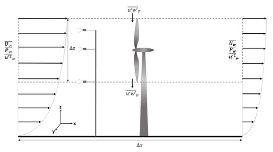
Figure 3.
A schematic of the wind turbine, the associated control volume within the ABL, and the variables required in Equation (7). The dashed rectangle depicts the control volume containing the wind turbine rotor.
- Mean flow only in the axial direction ()
- Homogeneity in the lateral direction ()
- Coriolis and gravitational forces are negligible
Expanding Equation (5), applying the above simplifications and rewriting as yields:
where is the wind turbine generated power per unit mass, is the turbulent component of axial wind speed, and is the turbulent component of vertical wind speed. It should be noted that the assumption of lateral homogeneity results in neglecting the lateral turbulent momentum flux in Equation (6) (), which is in agreement with the results reported by Cortina et al. [16]. They reported that almost all the lateral turbulent momentum flux that enters the control volume on one side, leaves the control volume on the other side. Considering the control volume in Figure 3, the gradient terms in Equation (6) are approximated, resulting in the following:
where subscript ∞ denotes flow conditions at the inflow, subscript w denotes flow conditions at the far wake, is the vertical turbulent momentum flux at the top of the control volume, is the vertical turbulent momentum flux at the bottom of the control volume, is the length of the control volume in the axial direction, and is the height of the control volume. Furthermore, we can assume that pressure far upstream of the wind turbine and far downstream of the wind turbine are equal to the undisturbed static pressure (). Therefore, we can neglect the pressure gradient in the axial direction, for the control volume in Figure 3. Applying this assumption to Equation (7) results in the following:
The wind turbine extracts energy from wind within a stream-tube shown in Figure 4, where subscript d denotes conditions right at the turbine cross-section. The presence of the wind turbine induces a wind speed component in the opposite direction of the incoming flow. Therefore, wind speed at the turbine cross-section is lower than inflow and continues to decrease in the axial direction in the wake area. In order for mass conservation to hold, the cross-sectional area of the stream-tube needs to increase in the axial direction, as shown in Figure 4. The magnitude of the decrease in wind speed at the turbine cross-section can be characterized by introducing a variable called axial flow induction factor, expressed as [30]:
Equation (9) combined with Bernoulli’s equation for upstream and downstream sections of the stream-tube results in the following relations between wind speed at the inflow and the far wake:
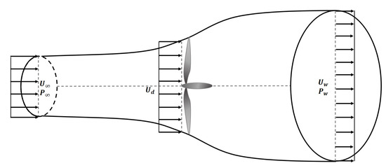
Figure 4.
The stream-tube containing the wind turbine expands in the axial direction due to the fact that wind speed decreases gradually from the inflow towards the far wake.
Furthermore, we can assume that wind speed at the turbine () represents the whole control volume and replace with in Equation (8), and multiply both sides of the equation by density and volume of the control volume (), in order to find the amount of power generated by the wind turbine:
where is the total power output of the turbine, A is the area swept by the rotor, and is the projected area of the control volume on the x-y plane. Substituting Equations (10) and (11) into Equation (12), and denoting as results in the following equation:
An equivalent wind speed that combines the effect of mean and turbulent parts of the wind speed can be defined as follows:
The value of can change with height due to wind shear. Therefore, we can quantify at several heights and integrate it vertically over the rotor swept area, which results in a rotor equivalent wind speed similar to the approach proposed in [5,8]:
where n is the number of heights at which wind speed is measured, h denotes each specific height, and is the portion of the rotor area corresponding to the height where the wind speed measurement is taken. Substituting Equations (14) and (15) into Equation (13) results in the following equation for the wind turbine power:
A power coefficient is defined as follows:
Taking the derivative of with respect to a and setting it to zero, results in the maximum theoretical value of 0.593 for the power coefficient, known as Betz’ limit. Replacing power coefficient into Equation (16) yields:
Furthermore, Equation (16) can be rewritten as a cubic function for axial flow induction factor, as follows:
Solving Equation (19) for a, and similar to the idea of power curves, an axial flow induction factor (induction curve for conciseness) can be introduced. The induction curve is produced by fitting a curve to bin-averaged values of axial flow induction factor with respect to rotor equivalent wind speed. Figure 5 shows an example induction curve fitted to data points averaged in bins of 0.5 m s−1. In turn, the induction curve in combination with Equation (16) can be used for prediction of power generation from a wind turbine. It can be observed that neglecting the turbulent terms in Equation (18), produces the same result as Equation (1), a well-known relation upon which power curves are based.
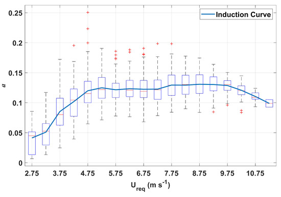
Figure 5.
An example induction curve for the 2.5 MW turbine in this study, derived using bins of 0.5 m s−1. The boxes show the interquartile range for each bin, the lower and upper quartiles are shown with dashed lines, and values outside the lower and upper qartiles are shown with red plus marks.
3. Data Sources
The wind power generation data considered in this study belongs to a stand-alone wind turbine, built in 2012 on the northeastern part of Kirkwood Community College in Cedar Rapids, Iowa (Figure 6). However, the atmospheric data used for characterizing the ABL come from a tall meteorological evaluation tower (met tower) located at an approximate distance of 900 m south of the wind turbine. The period of study spans from 20 February to 18 June 2018. More information about this site can be found in [2].
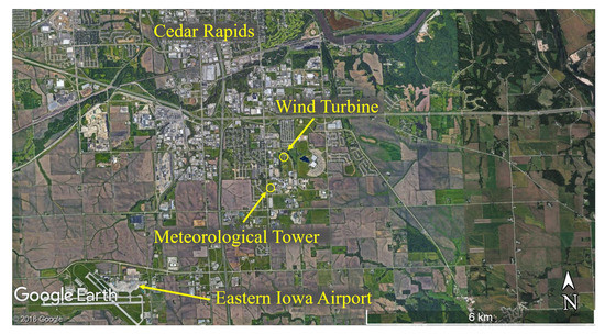
Figure 6.
Satellite image of the location of the 106 m tall met tower and the stand-alone wind turbine in relation to each other and the City of Cedar Rapids. Image: Google.
3.1. Wind Turbine SCADA System
The three-bladed, horizontal axis wind turbine considered in this study is a Clipper Liberty 2.5 MW turbine, is pitch-regulated, and has a hub-height of 80 m and a rotor diameter of 96 m. The rated power of the turbine was reduced to 2.3 MW by the operator for maintenance considerations. The cut-in wind speed of the turbine is 2.5 m s−1 and reaches its rated power at 13.5 m s−1 (Figure 1). The available data from the SCADA system includes wind speed, temperature, pressure, turbine orientation, power output and further wind turbine operational data, recorded as ten-minute averages.
3.2. Meteorological Tower Data
To measure the atmospheric conditions and the velocity profile of the incoming wind at the site, a 106 m tall meteorological tower was instrumented with sonic and cup anemometers, and wind vanes -among other sensors- at several heights in August 2017. A complete list of the instruments installed on the met tower is provided in Table 1. The sensors are mounted on seven horizontal booms, located at six different heights. At the top of the met tower, two booms extend in opposite directions for redundancy.

Table 1.
List of the sensors installed on the met tower.
The wind turbine and the met tower are both located on the southeastern side of the city of Cedar Rapids, while the wind turbine is located on the northeastern side of the met tower. Figure 6 shows a satellite image of the site of the wind turbine, the surrounding landscape and complexities of the land cover at this site. The north and northwest side of the site include suburban areas associated with higher roughness lengths, while east, south and southwestern parts of the site include agricultural lands associated with lower roughness lengths.
A schematic of the met tower and the instruments installed is shown in Figure 7. All booms are instrumented with cup anemometers and wind vanes, in order to characterize the velocity profile within the atmospheric boundary layer. Booms 1–6 extend west, whereas Boom 7 extends east at the top of the tower. Boom 4 is aligned with the lower tip of the rotor (32 m), Boom 5 coincides with the hub-height (80 m) and Boom 6 is at the top of the tower (106 m). These three booms along with Boom 2 (10 m) are equipped with sonic anemometers and are 21 feet long, while the other booms are shorter and extend for 12 feet. For characterization of the wind profile at the inflow, sonic anemometers, wind vanes, temperature, and relative humidity sensors at heights 32 m, 80 m, and 106 m are considered in the models.
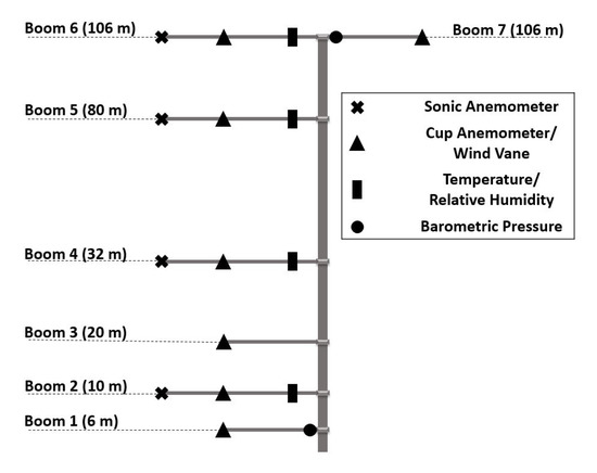
Figure 7.
A schematic of the sensors installed on the 106 m tall met tower at the site. The instruments are installed on seven booms, at six different heights. Six booms are extended towards the west while Boom 7 extends easterly.
3.3. Data Quality Control
Several quality checks are implemented on the dataset, in order to remove periods during which the data from either the met tower or SCADA system are not of sufficiently high quality. Description of these quality checks is provided in the following sections.
3.3.1. Quality Checks for Meteorological Tower Data
Data from the met tower were screened to ensure sufficient quality to be used in the models and measurements that are deemed of low quality are discarded. Sonic anemometers cannot measure wind speed under non-ideal conditions such as during precipitation, hence data points that are associated with such conditions are flagged and discarded. Another criterion is the measurement limits of the instruments provided by the manufacturers, thus data points that fall out of the measurement range of the sensors are also flagged and removed from the analysis. Furthermore, any spikes detected in the measurements are discarded. Fluctuations of excessively large amplitude for a very short duration are considered spikes, which can result from random electronic malfunctions of the sensors [33]. In this study, measurements that fall beyond 5 times the standard deviation during a thirty-minute period are flagged as spikes, and are removed from the analysis [33,34,35]. The aforementioned criteria are implemented for flagging low quality data, then any period whose flagged data points exceed 5% is discarded, similar to the approach employed in [12]. Application of these flagging criteria, results in the elimination of approximately 10% of the data (1800 ten-minute data points).
Measurements at the met tower are used in order to characterize inflow conditions into the wind turbine; however these measurements might not accurately represent wind flow conditions at the wind turbine due to the complexities of the terrain and structures surrounding the wind turbine and the met tower. Nacelle measurements are also corrected based on guidelines in [21] for accurately representing free flow conditions. Therefore, measurements at the met tower and at the nacelle of the wind turbine are compared and the following quality checks are performed.
The distribution of wind direction and energy generation based on ten-minute SCADA measurements are shown in Figure 8, and the dominant winds are from east, south and northwest, coinciding with dominant energy generation directions. The energy generation rose in Figure 8b shows the total amount of energy generated during the four-month period of study from different directions. Wind blowing from northeast, places the met tower in the wake of the turbine, hence met tower measurements under this condition do not accurately characterize the inflow conditions and are therefore removed from the analysis. Furthermore, analyzing the data showed that winds coming from east exhibit a shadowing effect by the met tower on flux measurements from the sonic anemometers, and the topography and surrounding buildings at the site causes negative shear—for sonic anemometers at 32 m, 80 m and 106 m—when the wind blows directly from north. In order to avoid these conditions, winds blowing from 340°–180° are discarded in this study. Applying these criteria results in discarding an additional 58% of the data (10,800 ten-minute data points).
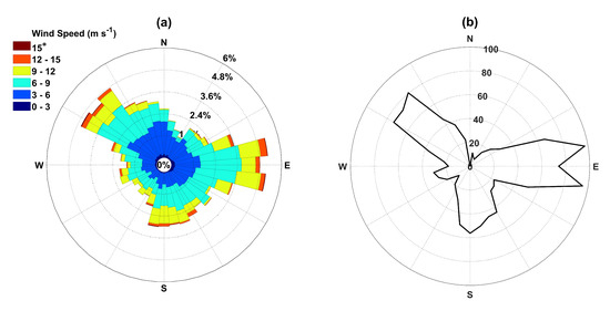
Figure 8.
Distribution of wind and generated energy during the four-month period of study: (a) wind rose from SCADA data and (b) energy rose from SCADA data in MWh, only for periods when the turbine was operating. The energy rose is generated by considering bins of 10°, and integrating the total amount of energy generated for each bin in MWh.
Moreover, data from the met tower need to be compared with nacelle measurements to make sure the wind profile at the met tower is the same as the one at the wind turbine. Li et al. [28] used a large-scale snow PIV system to characterize the induction zone for a wind turbine similar to the one in this study, and reported good agreement between wind speed at the nacelle and free flow. Furthermore, Smith et al. [36] studied wind turbines located in three different sites and found little difference between power prediction based on nacelle measurement and power prediction based on met tower measurement. In this study, hub-height wind speed measured at the met tower is compared to nacelle measurement, a 10% threshold is applied to the difference between the two measurements, and data not within this threshold are removed. After applying this criterion the coefficient of correlation between the two measurements for the remaining data points is 0.98, which is close to the values reported in [36]. The comparison of wind speed measured at the met tower against nacelle measurement is shown in Figure 9.
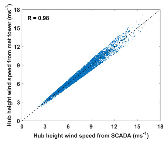
Figure 9.
Comparison of ten-minute averaged hub-height wind speed measurements at the met tower and at the nacelle. The diagonal represents a 1:1 relationship.
3.3.2. Quality Checks for SCADA Data
Data from the SCADA system is quality checked, and data points whose reported turbine power generation is significantly different than predicted from power curve are discarded. This difference in power generation could be due to several reasons including the generator not being operational, the rated power being set below 2.3 MW, the grid being out of operational range, or the wind turbine undergoing maintenance service. St Martin et al. [12] proposed two different approaches to find such data points, blade pitch angle variations and turbine operational parameters, while the latter approach proved to be more efficient in finding periods when turbine is producing less power than expected, hence this approach is implemented in this study. The combination of all these filters results in discarding 18% of the original dataset (3437 ten-minute data points). Overall, implementing all of the quality checks described in previous sections, results in 14% of the original dataset to be used in the evaluation of the model (2274 ten-minute data points, equivalent to approximately 16 days).
4. Discussion of the Results
The process through which the axial flow induction factor curve, described in Section 2.3, is applied to the data is explained in this section. The model is implemented for wind turbine power prediction, and the accuracy of the results from this model is compared to the standard power curve and the recently proposed power surface model. At wind speeds of 11 m s−1 and above, transition to the rated power region of the power curve occurs, where power generation is constant. In this study we only focus on the operational region of the power curve and wind speeds lower than 11 m s−1, and compare the results of the models for this range of wind speeds.
Figure 10 shows the distribution of key atmospheric variables including air density, turbulence intensity, and wind shear, upon which—along with wind speed-power is dependent. The variability of these parameters at the site, suggests that including them in any model for forecasting wind power can improve the accuracy of the prediction.
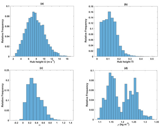
Figure 10.
Observed distribution of ten-minute averaged atmospheric variables, including: (a) hub-height wind speed (m s−1), (b) hub-height turbulence intensity (), (c) shear exponent, (d) hub-height air density (kg m−3).
Figure 10a shows the distribution of wind speed at hub-height from SCADA, which resembles a normal distribution with a mean value of 7.7 m s−1 during the four-month period of study. It should be noted that this value is greater than the ten-year average wind speed at this site, based on measurements at Eastern Iowa Airport corrected for hub-height, located approximately 5 km from the site [26]. Another important atmospheric variable for prediction of wind turbine power is turbulence intensity (), which has been reported to have a significant effect on power prediction accuracy in [4]. The distribution of is shown in Figure 10b, and it is defined as:
where is the standard deviation of hub-height wind speed, and U is ten-minute averaged hub-height wind speed. Furthermore, hub-height wind speed does not necessarily represent wind flow across the rotor swept area, due to wind shear. A measure to quantify this change is the shear exponent , defined based on power law profile for wind:
where is the ten-minute averaged wind speed and z is the height at which wind speed is measured. Figure 10c shows the distribution of shear exponent at the site, and is based on sonic anemometer measurement of wind speed at heights 32 m, 80 m and 106 m. The range of observed values of at this site are higher than the ranges reported in [12,23], which can be contributed to the suburban landscape of the site, and larger size of the turbine in this study.
Furthermore, air density is an important variable for wind turbine power prediction, since it is linearly related to power, as shown in Equation (1). Air density shown in Figure 10d exhibits a bi-modal distribution at this site with a mean value of 1.19 kg m−3. Including the atmospheric variables shown in Figure 10 in the standard power curves, improves the accuracy of power prediction from wind turbines. Additionally, the approach described in Section 2.3 which results in Equation (16), would allow the inclusion of turbulent fluxes of energy in power prediction, as well. Solving the cubic function in Equation (19) for each ten-minute period, results in three different possible values for the axial flow induction factor during that ten-minute window. However, values of axial flow induction factor equal to 0.5 or greater are discarded, since they result in zero or negative downstream velocity (based on Equation (11)). In the case of this study, of the three possible values for a, only one is less than 0.5 for all data points used in the analysis.
The challenge with solving Equation (19) is that the value of the area of horizontal projection of the control volume () is also unknown (Figure 3). Moreover, previous studies [15,16,17] suggest that vertical turbulent momentum flux changes in the axial direction. Therefore, the value of vertical turbulent momentum flux measured at the met tower does not necessarily represent the entire control volume. In order to approximate the integrated value of vertical turbulent momentum flux over the control volume, we propose making the following assumption:
where is the gradient of vertical turbulent momentum flux in the vertical direction at the inflow (met tower) and is a coefficient used to correct for the planar average flux across the top and bottom surfaces of the control volume. Substituting Equation (22) into Equation (19) yields:
Values of both a and are unknown in Equation (23). Therefore, solving this equation for each ten-minute period requires an iterative procedure in which an initial value for is assumed, then Equation (23) is solved for a, an induction curve is created for each value of , and the one that results in the most accurate power prediction is chosen. The induction curve is created similar to the standard power curve. The values of a obtained from Equation (23) and for a fixed value of are divided into bins of 0.5 m s−1, and a curve is fitted to the bin-averaged values of axial flow induction factor. Figure 11 depicts the induction curve that results from this bin-averaging procedure, for wind speeds up to 11 m s−1, the operational range for the turbine in this study.
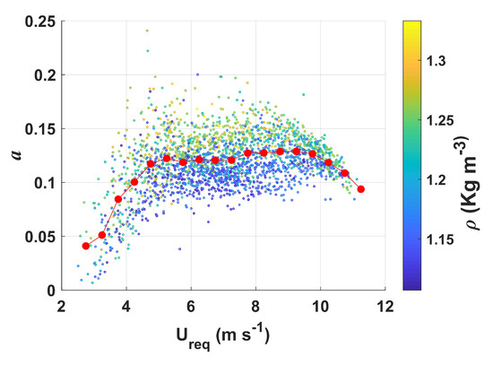
Figure 11.
Variation of induction factor with wind speed and density, as derived from Equation (23), based on 10 min mean wind speed and turbulent flux data. An Induction curve is obtained using bins of 0.5 m s−1 for .
The induction curve shown in Figure 11 can now be used for prediction of wind turbine power generation. In other words, knowing the value of rotor equivalent wind speed, the value of a is derived from the induction curve in Figure 11, then it is substituted into Equation (16) to get the power generation. Root mean square error () and mean absolute error () are implemented as measures for accuracy of power prediction, which are defined as follows:
where is the actual power and is the predicted power. Smaller values of and represent higher accuracy in the prediction model while greater values of and indicate less accurate power prediction.
As mentioned earlier, the value of is unknown and the induction curve changes based on different values of . Therefore, we use an iterative procedure in which an initial value for is assumed, then the induction curve is formed, the resulting induction curve is used to predict the wind turbine power generation, and finally the corresponding values for and are found. This procedure is repeated to find the value for which minimizes and . Furthermore, Cortina et al. [16,17] showed that the axial changes in vertical turbulent momentum flux depend on thermal stability. Therefore, the iterative procedure for finding is repeated for different stability regimes. Stability regimes may be characterized by several measures. Here we chose Bulk Richardson number () which is calculated from the ratio of buoyant forces to shear forces, as follows [37]:
where g is the gravitational acceleration (9.81 m s−2), is the vertical change in temperature, is the change in height and is the average temperature over . For quantifying , measurements at the lower tip of the rotor (32 m) and the top of the met tower (106 m) are used to represent stability conditions across the rotor swept area. For classifying stability regimes, the distribution of is divided into three subsets of roughly the same size. This approach is similar to the one proposed in [12,38] and results in a better separation between stable and unstable regimes [12]. Figure 12 shows the classification of stability regimes based on distribution, where neutral conditions correspond to the range .
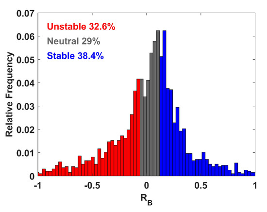
Figure 12.
Classification of stability regimes based on distribution of .
Once the classification of stability regimes is performed, the value of is determined for each stability regime. Figure 13 shows the results for for different stability regimes. For stable conditions shown in Figure 13a, the value of has less impact on , compared to both neutral and unstable conditions, with the optimum value of also having a smaller magnitude than the other two cases, which shows that for stable conditions vertical turbulent fluxes are not as important as neutral and unstable conditions in power prediction. Taking the values of found in Figure 13, and substituting them into Equation (23) results in a more accurate induction curve, which is shown in Figure 14a.
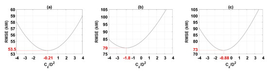
Figure 13.
The effect of on of power prediction showing optimum values for: (a) stable regime, (b) neutral regime, (c) unstable regime, normalized by , where D is the diameter of the wind turbine.
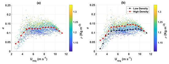
Figure 14.
(a) Induction curve resulting from values of found for different stability regimes and then dividing axial flow induction factor values into bins of 0.5 m s−1 for and (b) two induction curves resulting from division of data into two smaller sets based on air density.
However, a closer look at Figure 14a reveals a relation between axial flow induction factor and air density; lower air density results in lower axial flow induction factor, and vice versa. Since Figure 10d exhibits a bi-modal distribution of air density at this site, and in order to take into account the effect of air density on induction curve, we divide the dataset into two halves based on air density, then create an induction curve for each smaller subset. The resulting two induction curves are shown in Figure 14b.
The induction curves in Figure 14 can be used in combination with Equation (16) for power prediction. From this point forward, we refer to the curve in in Figure 14a as the induction curve model and the curves in Figure 14b as double induction curve model. Figure 15 shows the performance of these two models compared to the standard power curve and the power surface model, when applied to the same dataset. The x-axis represents actual power output from the turbine, and the predicted power output is plotted on the y-axis. Subsequently, a perfect power prediction should fall on the 1:1 line on the diagonal. Moreover, the color bar shows the turbulence intensity, with brighter colors representing higher values of turbulence intensity. In all models, there is a high concentration of low turbulence intensity data points above the diagonal.
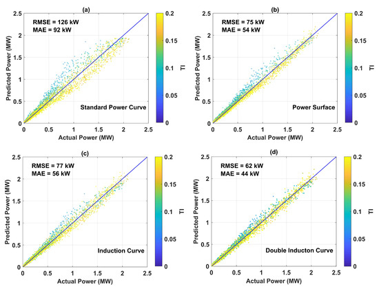
Figure 15.
Performance of: (a) standard power curve, (b) power surface, (c) induction curve, and (d) double induction curve, for predicting power generation of the wind turbine.
Figure 15 also shows that all three models perform significantly better than the standard power curve. Visual inspection of this figure reveals that the amount of digression from the diagonal line decreases from Figure 15a–d, qualitatively implying improvement in power prediction using these models. In order to quantify the amount of improvement in power prediction, we look at and values for all models. All three models result in smaller error values for power prediction, while the power surface and induction curve resulting in very similar accuracy, and the double induction curve resulting in the most accurate power prediction. The standard power curve results in error values of = 126 kW and = 92 kW, as shown in Figure 15a. The power surface and induction curve models shown in Figure 15b,c, demonstrate similar accuracy in power prediction, with = 75 kW and = 54 kW for power surface and = 77 kW and = 56 kW for induction curve. Subsequently, the power surface and induction curve achieve 40% and 39% improvement in accuracy of power prediction, respectively, in terms of both and . Furthermore, Figure 15d shows the performance of the double induction curve model, which results in = 62 kW and = 44 kW, a significant, 51% and 52%, reduction in power prediction error compared to the standard power curve in terms of and , respectively. The similar accuracy of the power surface and induction curve models for the stand-alone turbine considered for this study is an interesting observation. Further analysis of these models for wind turbines located in complicated ABL flows and within wind farms will provide better understanding of the performance of these two models.
Figure 16 shows the error reduction from double induction curve and power surface models during a sample twelve-hour period on 16 February 2018 from 3:00 a.m. to 3:00 p.m., when the average values of both turbulence intensity (0.16) and air density (1.27 kg m−3) were high. During the visualized twelve-hour period and compared to the standard power curve, the average absolute error for power prediction from the double induction curve and the power surface models are reduced by 75% and 72%, respectively. The of power prediction during this period is approximately 58 kW, 64 kw, and 230 kW for the double induction curve, power surface and standard power curve, respectively.
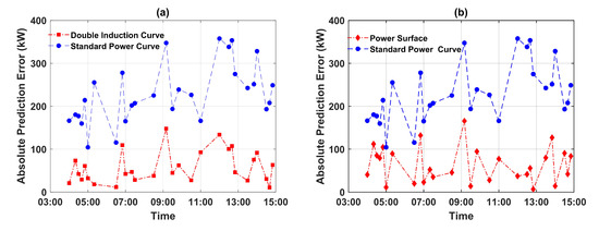
Figure 16.
Time series of error reduction in power prediction during a sample twelve-hour period on 16 February 2018 from 3:00 a.m. to 3:00 p.m., resulting from (a) double induction curve, and (b) power surface, compared to the standard power curve.
Approximation of Turbulent Momentum Fluxes
Once induction curve and double induction curves are derived for a wind turbine at a site, the application of these models to power prediction requires quantifying vertical turbulent momentum fluxes using high-resolution instruments such as sonic anemometers. However, three-dimensional data for wind speed at several heights are usually not available, hence direct quantification of turbulent momentum fluxes is a challenge. An alternative approach is to approximate turbulent fluxes by means of using the stream-wise variance of wind speed as a surrogate, which has been investigated in the literature [39,40,41,42,43,44], along with the relations between other turbulent quantities. Figure 17 shows the linear relation between the variance of stream-wise wind speed and the turbulent vertical momentum flux, considering holds near the surface. This relationship is plotted at heights of 32 m, 80 m, and 106 m while setting the intercept to the origin.
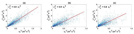
Figure 17.
The linear relation between and while setting the intercept to the origin, and for the sonic anemometers on (a) boom 4 (32 m), (b) boom 5 (80 m), and (c) boom 6 (106 m).
Similar to Figure 17 and results presented in [39], linear relationships between other turbulent quantities are found for the three sonic anemometers at heights 32 m, 80 m, and 106 m. These linear relationships are summarized in Table 2, with the last row representing the average value of the three aforementioned sonic anemometers at this site. As can be seen in Table 2, the values found in this study are in good agreement with previous results, and in particular with values from Lenschow et al. [41]. Similar to this study, Lenschow et al. conducted their study at a site characterized as rolling terrain, and measured turbulent quantities at several heights. Detailed analysis of relations between turbulent quantities is not the focus of this study, and for approximating the value of vertical turbulent momentum flux (), we only need the relation between the variance of stream-wise wind speed () and vertical turbulent momentum flux () provided in the first column of Table 2, and the rest of the columns are provided only for comparison with findings in previous studies.
Table 2.
Relations between different turbulent quantities, as reported in [39].
Figure 17 and Table 2 provide a relation through which we can approximate the value of vertical turbulent momentum flux using variance of the stream-wise wind speed, and use it in combination with Equation (16) and the induction curve models for power prediction. This approach can be used when direct measurements of turbulent fluxes are not available.
Figure 18 shows the performance of the induction curve and double induction curve models using approximated values of the turbulent fluxes. The approximation of vertical turbulent fluxes in both induction curve and double induction curve models results in prediction errors much lower than standard power curves. However, it should be noted that for a stand-alone wind turbine the contribution of vertical turbulent fluxes to power generation is significantly smaller than mean axial fluxes as presented in [15,16,17]. For the four-month period of study, the average value of this contribution was 2%. Therefore, the small difference in prediction error shown in Figure 18 is partly due to the small contribution of turbulent fluxes to power generation. On the other hand, for a wind turbine in the middle of a wind farm, the contribution of turbulent fluxes to power generation could increase to the same order of magnitude as mean axial fluxes [15], thus a detailed study of such wind turbines is needed in order to have a better understanding of the performance of induction curve and double induction curve models, using direct and approximated values of turbulent fluxes.
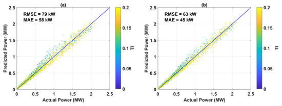
Figure 18.
Performance of: (a) induction curve using approximated values of turbulent fluxes, and (b) double induction curve using approximated values of turbulent fluxes, for predicting power generation of the wind turbine.
5. Concluding Remarks and Future Work
Data from a met tower and SCADA system of a 2.5 MW horizontal axis wind turbine were analyzed during a period of four months, in order to develop new models for predicting wind power generation. The proposed approach uses a curve for axial flow induction factor, instead of the standard power curve generally used for the purpose of power prediction. The proposed induction curve takes into account the effect of mean wind speed, wind speed variations, wind shear, density variations, thermal stability, and vertical turbulent momentum fluxes on wind turbine power generation.
The wind turbine and the met tower are located near the suburban area of the city of Cedar Rapids, Iowa, and due to the complexities of the site and local variation in the landscape, a full characterization of the ABL at the inflow of the wind turbine using the met tower is not possible. Hence, data from the met tower were filtered carefully considering various quality checks, to accurately represent the atmospheric conditions at the inflow of the wind turbine and were used in the power prediction models. The proposed induction curves were compared to the standard power curve in terms of and of power prediction. The results show that both power surface and induction curve models perform better than the standard power curve, while the double induction curve model can reduce power prediction error as much as 75% as demonstrated for a sample twelve-hour period. The contribution of vertical momentum fluxes to power generation at this site proved to be small, representing 2% of the total power generation on average. Such a small contribution is expected, as the focus of this study was on a stand-alone wind turbine. However, this contribution is expected to be significantly higher in complex flows such as a wind farm, and be as high as 79% of the total generated power as reported in [15,16]. It should be noted that ten-minute averaging periods are normally used in wind power analysis. Therefore, momentum fluxes and turbulent quantities in this study are defined over ten-minute periods. However, turbulence in the ABL is usually measured over longer averaging windows.
It was also concluded that all models generally over-predict power generation when turbulence intensity is low, and under-predict power generation when turbulence intensity is high. Therefore, the effect of turbulence intensity is not completely understood and needs to be investigated further. Moreover, the use of approximated values for vertical turbulent fluxes in the models as opposed to direct measurement showed promising results. Furthermore, a full quantification of axial variations of vertical turbulent momentum flux along the control volume, especially near the turbine will be helpful in understanding the contribution of this term to power generation. Lastly, this study was performed on a stand-alone wind turbine. In the future, a similar study on a wind turbine within a wind farm is needed for full assessment of the performance of the proposed approach.
Author Contributions
M.V. collected the data, implemented the codes for data preparation and analysis of the models. Discussion and analysis of results was performed by M.V. and C.D.M.; All authors have read and agreed to the published version of the manuscript.
Funding
National Science Foundation Iowa EPSCoR Grant Number: 1101284; Center for Global & Regional Environmental Research (CGRER), University of Iowa.
Acknowledgments
The authors would like to thank Kirkwood Community College for their cooperation and allowing access to the SCADA data. We also extend our appreciation to Clipper Windpower for granting access to technical data on the Liberty wind turbine. This research was funded by National Science Foundation Iowa EPSCoR (Grant No 1101284) and Center for Global & Regional Environmental Research (CGRER), University of Iowa.
Conflicts of Interest
The authors declare no conflict of interest.
References
- Edenhofer, O.; Pichs-Madruga, R.; Sokona, Y.; Seyboth, K.; Kadner, S.; Zwickel, T.; Eickemeier, P.; Hansen, G.; Schlömer, S.; von Stechow, C.; et al. Renewable Energy Sources and Climate Change Mitigation: Special Report of the Intergovernmental Panel on Climate Change; Cambridge University Press: Cambridge, UK, 2011. [Google Scholar]
- Vahidzadeh, M.; Markfort, C.D. Modified Power Curves for Prediction of Power Output of Wind Farms. Energies 2019, 12, 1805. [Google Scholar] [CrossRef]
- Würth, I.; Valldecabres, L.; Simon, E.; Möhrlen, C.; Uzunoğlu, B.; Gilbert, C.; Giebel, G.; Schlipf, D.; Kaifel, A. Minute-scale forecasting of wind power—Results from the collaborative workshop of IEA Wind task 32 and 36. Energies 2019, 12, 712. [Google Scholar] [CrossRef]
- Clifton, A.; Kilcher, L.; Lundquist, J.; Fleming, P. Using machine learning to predict wind turbine power output. Environ. Res. Lett. 2013, 8, 024009. [Google Scholar] [CrossRef]
- Wagner, R.; Courtney, M.; Gottschall, J.; Lindeløw-Marsden, P. Accounting for the speed shear in wind turbine power performance measurement. Wind Energy 2011, 14, 993–1004. [Google Scholar] [CrossRef]
- Choukulkar, A.; Pichugina, Y.; Clack, C.T.; Calhoun, R.; Banta, R.; Brewer, A.; Hardesty, M. A new formulation for rotor equivalent wind speed for wind resource assessment and wind power forecasting. Wind Energy 2016, 19, 1439–1452. [Google Scholar] [CrossRef]
- Kaiser, K.; Langreder, W.; Hohlen, H.; Højstrup, J. Turbulence correction for power curves. In Wind Energy; Springer: Berlin/Heidelberg, Germany, 2007; pp. 159–162. [Google Scholar]
- Wagner, R.; Antoniou, I.; Pedersen, S.M.; Courtney, M.S.; Jørgensen, H.E. The influence of the wind speed profile on wind turbine performance measurements. Wind Energy 2009, 12, 348–362. [Google Scholar] [CrossRef]
- Langreder, W.; Kaiser, K.; Hohlen, H.; Hojstrup, J. Turbulence Correction for Power Curves; EWEC: London, UK, 2004. [Google Scholar]
- Tindal, A.; Johnson, C.; LeBlanc, M.; Harman, K.; Rareshide, E.; Graves, A. Site-specific adjustments to wind turbine power curves. In Proceedings of the AWEA Wind Power Conference, Houston, TX, USA, 1–4 June 2008. [Google Scholar]
- Albers, A.; Jakobi, T.; Rohden, R.; Stoltenjohannes, J. Influence of meteorological variables on measured wind turbine power curves. In Proceedings of the European Wind Energy Conf. & Exhibition, Berlin, Germany, 4–6 December 2007; pp. 525–546. [Google Scholar]
- St Martin, C.M.; Lundquist, J.K.; Clifton, A.; Poulos, G.S.; Schreck, S.J. Wind turbine power production and annual energy production depend on atmospheric stability and turbulence. Wind Energy Sci. (Online) 2016, 1. [Google Scholar] [CrossRef]
- Wharton, S.; Lundquist, J.K. Atmospheric stability affects wind turbine power collection. Environ. Res. Lett. 2012, 7, 014005. [Google Scholar] [CrossRef]
- Redfern, S.; Olson, J.B.; Lundquist, J.K.; Clack, C.T. Incorporation of the Rotor-Equivalent Wind Speed into the Weather Research and Forecasting Model’s Wind Farm Parameterization. Mon. Weather Rev. 2019, 147, 1029–1046. [Google Scholar] [CrossRef]
- Lebron, J.; Castillo, L.; Meneveau, C. Experimental study of the kinetic energy budget in a wind turbine streamtube. J. Turbul. 2012, 13, N43. [Google Scholar] [CrossRef]
- Cortina, G.; Calaf, M.; Cal, R.B. Distribution of mean kinetic energy around an isolated wind turbine and a characteristic wind turbine of a very large wind farm. Phys. Rev. Fluids 2016, 1, 074402. [Google Scholar] [CrossRef]
- Cortina, G.; Sharma, V.; Calaf, M. Wind farm density and harvested power in very large wind farms: A low-order model. Phys. Rev. Fluids 2017, 2, 074601. [Google Scholar] [CrossRef]
- Markfort, C.D.; Zhang, W.; Porté-Agel, F. Turbulent flow and scalar transport through and over aligned and staggered wind farms. J. Turbul. 2012, 13, N33. [Google Scholar] [CrossRef]
- IEC. International Standard, Wind Turbines-Part 12-1: Power Performance Measurements of Electricity Producing Wind Turbines; IEC 61400-12-1; International Electrotechnical Commission: Geneva, Switzerland, 2005. [Google Scholar]
- Betz, A. Schraubenpropeller mit geringstem Energieverlust. Gottinger Nachrichten 1919, 1919, 193–213. [Google Scholar]
- Commission, I.E. Power Performance of Electricity Producing Wind Turbines Based on Nacelle Anemometry; Technical Report, IEC 61400-12-2 CD Part 12-2; International Electrotechnical Commission: Geneva, Switzerland, 2008. [Google Scholar]
- Simley, E.; Angelou, N.; Mikkelsen, T.; Sjöholm, M.; Mann, J.; Pao, L.Y. Characterization of wind velocities in the upstream induction zone of a wind turbine using scanning continuous-wave lidars. J. Renew. Sustain. Energy 2016, 8, 013301. [Google Scholar] [CrossRef]
- Bulaevskaya, V.; Wharton, S.; Clifton, A.; Qualley, G.; Miller, W. Wind power curve modeling in complex terrain using statistical models. J. Renew. Sustain. Energy 2015, 7, 013103. [Google Scholar] [CrossRef]
- Iungo, G.V. Experimental characterization of wind turbine wakes: Wind tunnel tests and wind lidar measurements. J. Wind Eng. Ind. Aerodyn. 2016, 149, 35–39. [Google Scholar] [CrossRef]
- Shin, D.; Ko, K. Application of the Nacelle Transfer Function by a Nacelle-Mounted Light Detection and Ranging System to Wind Turbine Power Performance Measurement. Energies 2019, 12, 1087. [Google Scholar] [CrossRef]
- Carbajo Fuertes, F.; Markfort, C.D.; Porté-Agel, F. Wind Turbine Wake Characterization with Nacelle-Mounted Wind Lidars for Analytical Wake Model Validation. Remote Sens. 2018, 10, 668. [Google Scholar] [CrossRef]
- Brugger, P.; Fuertes, F.C.; Vahidzadeh, M.; Markfort, C.D.; Porté-Agel, F. Characterization of Wind Turbine Wakes with Nacelle-Mounted Doppler LiDARs and Model Validation in the Presence of Wind Veer. Remote Sens. 2019, 11, 2247. [Google Scholar] [CrossRef]
- Li, C.; Abraham, A.; Li, B.; Hong, J. Investigation on the Atmospheric Incoming Flow of a Utility-Scale Wind Turbine using Super-large-scale Particle Image Velocimetry. arXiv 2019, arXiv:1907.11386. [Google Scholar]
- Dasari, T.; Wu, Y.; Liu, Y.; Hong, J. Near-wake behaviour of a utility-scale wind turbine. J. Fluid Mech. 2019, 859, 204–246. [Google Scholar] [CrossRef]
- Burton, T.; Jenkins, N.; Sharpe, D.; Bossanyi, E. Wind Energy Handbook; John Wiley & Sons: Hoboken, NJ, USA, 2011. [Google Scholar]
- Markfort, C.D.; Zhang, W.; Porté-Agel, F. Analytical model for mean flow and fluxes of momentum and energy in very large wind farms. Bound.-Layer Meteorol. 2018, 166, 31–49. [Google Scholar] [CrossRef]
- Tennekes, H.; Lumley, J.L.; Lumley, J. A First Course in Turbulence; MIT Press: Cambridge, MA, USA, 1972. [Google Scholar]
- Lee, X.; Massman, W.; Law, B. Handbook of Micrometeorology: A Guide for Surface Flux Measurement and Analysis; Springer: Berlin/Heidelberg, Germany, 2004; Volume 29. [Google Scholar]
- Mauder, M.; Foken, T. Documentation and Instruction Manual of the Eddy-Covariance Software Package TK3 (Update); University of Bayreuth: Bayreuth, Germany, 2015. [Google Scholar]
- Aubinet, M.; Vesala, T.; Papale, D. Eddy Covariance: A Practical Guide to Measurement and Data Analysis; Springer: Berlin/Heidelberg, Germany, 2012. [Google Scholar]
- Smith, B.; Link, H.; Randall, G.; McCoy, T. Applicability of Nacelle Anemometer Measurements for Use in Turbine Power Performance Tests; Technical Report; National Renewable Energy Lab.: Golden, CO, USA, 2002. [Google Scholar]
- Stull, R.B. An Introduction to Boundary Layer Meteorology; Springer: Berlin/Heidelberg, Germany, 2012; Volume 13. [Google Scholar]
- Aitken, M.L.; Banta, R.M.; Pichugina, Y.L.; Lundquist, J.K. Quantifying wind turbine wake characteristics from scanning remote sensor data. J. Atmos. Ocean. Technol. 2014, 31, 765–787. [Google Scholar] [CrossRef]
- Banta, R.M.; Pichugina, Y.L.; Brewer, W.A. Turbulent velocity-variance profiles in the stable boundary layer generated by a nocturnal low-level jet. J. Atmos. Sci. 2006, 63, 2700–2719. [Google Scholar] [CrossRef]
- Nieuwstadt, F.T. The turbulent structure of the stable, nocturnal boundary layer. J. Atmos. Sci. 1984, 41, 2202–2216. [Google Scholar] [CrossRef]
- Lenschow, D.H.; Li, X.S.; Zhu, C.J.; Stankov, B.B. The stably stratified boundary layer over the Great Plains. In Topics in Micrometeorology. A Festschrift for Arch Dyer; Springer: Berlin/Heidelberg, Germany, 1988; pp. 95–121. [Google Scholar]
- Smedman, A.S. Observations of a multi-level turbulence structure in a very stable atmospheric boundary layer. Bound.-Layer Meteorol. 1988, 44, 231–253. [Google Scholar] [CrossRef]
- Berström, H.; Smedman, A.S. Stably stratified flow in a marine atmospheric surface layer. Bound.-Layer Meteorol. 1995, 72, 239–265. [Google Scholar] [CrossRef]
- Smedman, A.S.; Bergström, H.; Högström, U. Spectra, variances and length scales in a marine stable boundary layer dominated by a low level jet. Bound.-Layer Meteorol. 1995, 76, 211–232. [Google Scholar] [CrossRef]


© 2020 by the authors. Licensee MDPI, Basel, Switzerland. This article is an open access article distributed under the terms and conditions of the Creative Commons Attribution (CC BY) license (http://creativecommons.org/licenses/by/4.0/).