Time Domain Particle Swarm Optimization of PI Controllers for Bidirectional VSC HVDC Light System

Abstract

This paper proposes a novel technique to tune the PI controllers of a bidirectional HVDC light system by embedding particle swarm optimization directly in the Simulink model in the design procedure. The HVDC light system comprises of a rectifier station, a DC link, and an inverter station. Each converter station requires four PI controllers to be tuned in the decoupled d-q vector control scheme, and with the bidirectional HVDC system, the required PI controllers are doubled. Tuning these many controllers using conventional methods is a challenging task, especially if the parameters of the converter stations are different. A novel approach to tune the PI controllers for a bidirectional HVDC system using the time-domain performance indices is presented in this paper. The time-domain performance indices are optimized using the particle swarm optimization (PSO) algorithm. The results of the proposed tuning method show that the proposed method not only gives superior results but also is less cumbersome to tune compared to conventional methods like modulus optimum (MO).

1. Introduction

The brisk development of power electronic technology in recent years has led to the advancement of voltage source converters (VSC), which has resulted in a new era of HVDC light systems. This has renewed the interest of researchers in HVDC transmission. New challenges in the control design of HVDC light systems are encountered due to these rapid developments in technology [1,2]. The HVDC light systems connect AC systems and have converter stations on each side. The design of proper controllers for both the converter stations is of utmost importance to take full advantage of the HVDC light systems. Many control schemes have been reported in the literature for the HVDC light system [2,3,4,5,6,7,8,9,10,11,12,13,14,15]. In [2], control of the HVDC light system using conventional and direct-current vector control approaches is discussed. Robust sliding mode control, multivariable optimal control, and adaptive control for VSC-HVDC transmission are presented in [2,5,7,8,9]. Reference [10] discusses the principles of quasi optimum PI controller tuning rules for a grid-connected three phase AC to DC pulse width modulation (PWM) rectifier. In [7], the state-space model of the HVDC light transmission system is derived in d-q coordinate frame. The derived model is then linearized to obtain the small-signal model. Next, a multivariable optimal PI controller is designed for the small-signal model using a linear quadratic regulator (LQR). The dynamic model and control of AC–DC–AC voltage-sourced converter system for distributed resources is presented in [11].

The control technologies for the traditional thyristor based line commutated converters (LCC) HVDC systems are well established and have been in use for a long time [4]. These technologies cannot be directly applied to the VSC-based HVDC light system because the degrees of freedom presented by the VSC-based converters pose new challenges. The most common control strategies applied for VSC-based HVDC light systems are the voltage oriented control (VOC) and the direct power control (DPC). The VOC control strategy employs a decoupled nested-loop d-q vector control technique, whereas DPC utilizes a hysteresis controller [2,7]. Compared to DPC, VOC has fixed switching frequency and better utilization of DC bus voltage. In a decoupled nested loop d-q VOC, the inner loop controls the d-q currents, while the outer loops are used to control DC link voltage/active power and AC terminal voltage/reactive power for both control stations. PI controllers are mostly used in the decoupled nested loop vector control technique because of its simple structure and ease of implementation. There are four PI controllers at each converter station, so a typical bipolar bidirectional VSC-HVDC system that is shown in Figure 1 will have a total of sixteen PI controllers. Tuning methods like pole-zero cancellation using bode plots, pole placement, and Ziegler–Nichols are some of the widely used methods to tune PI controllers in cascaded loops. However, tuning based on these methods depends heavily on the system model and does not guarantee stability [8]. Thus, additional manual tuning using a trial and error method is required. Because of this, tuning sixteen PI controllers is a challenging and time consuming task. Additionally, these methods do not give optimal parameters, resulting in underutilization of the bandwidth of the system. Conventional optimal tuning methods like modulus optimum (MO) and symmetrical optimum (SO) are mostly applicable to systems with one large time constant and several small time constants and require simplified system models. Controllers tuned by MO and SO methods provide a good response with low overshoot, but the closed-loop system has poor rejection capability for disturbance [14]. Even though the tuning rules for PI parameters are well documented, they mostly rely on the designer’s experience, and moreover, the tuned PI controller does not guarantee optimal performance.

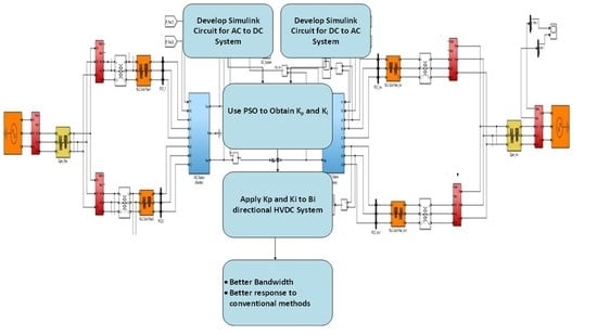
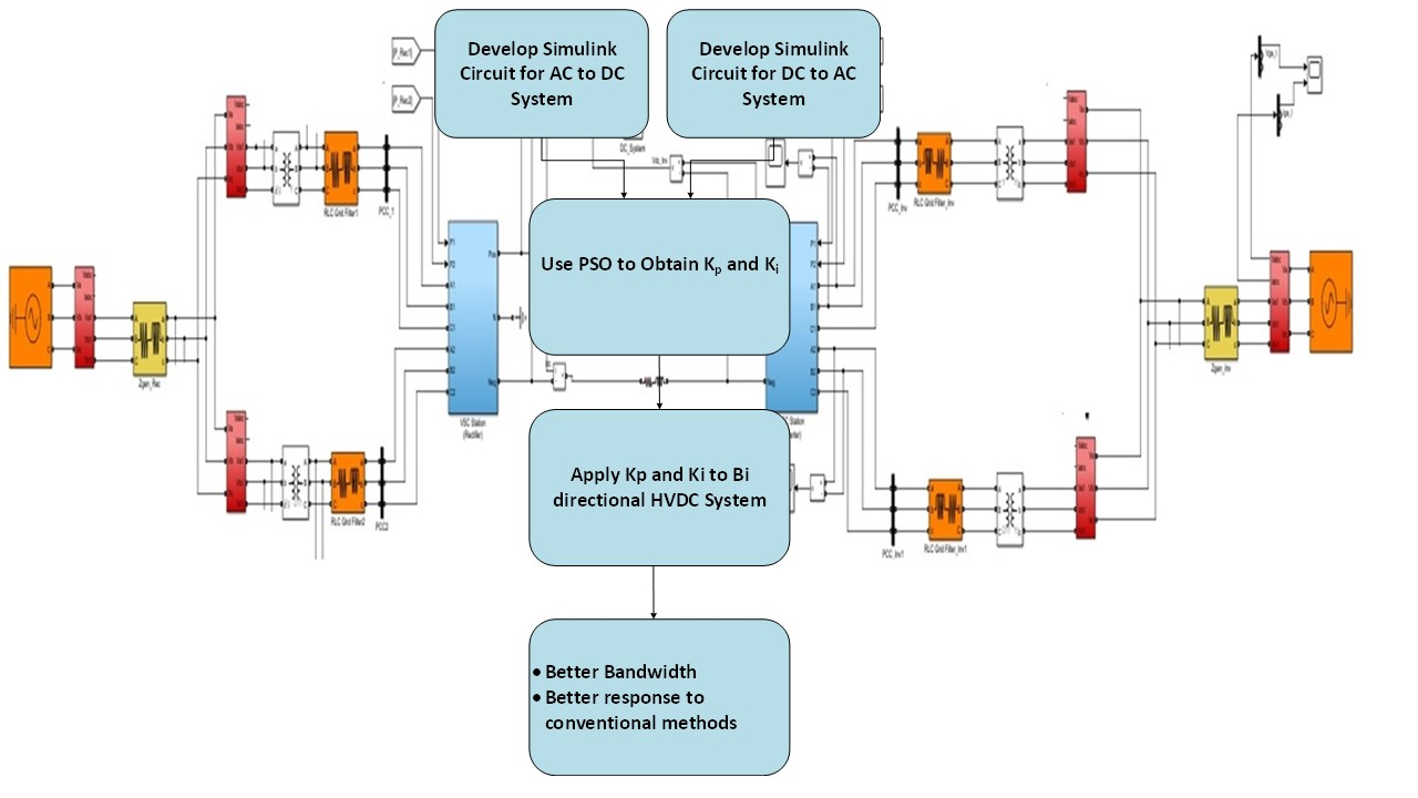
In spite of a large number of studies carried out in the field of control design for the HVDC light systems, certainly, there is still room for improvement in the way the controllers are designed and their parameters optimized. Tuning based on optimization algorithms like particle swarm optimization (PSO) [15,16,17] and genetic algorithm (GA) [18] and have been reported in the past. In [19], PSO is applied for multiterminal DC grids and it demonstrates a better performance of PSO over classical tuning. In these, a linearized and simplified model is used for tuning the controllers as it results in fast convergence. PSO is preferred over the other optimization techniques as it is simple to program and has a fast convergence rate. In this paper, PSO is used to tune the parameters of PI controllers for the bidirectional HVDC light system. The controller design is formulated as an optimization problem, and time-domain performance indices are used to optimize the parameters of the PI controllers. The novelty of the present paper is to embed the PSO algorithm in the controller design steps directly on the Simulink model, which include the detailed model of the switches and the nonlinear components of the power system. The existing PSO methods [15,19,20,21] use approximated model of the converters. Therefore, the proposed approach results in a more realistic representation of the actual system. The time-domain performance index that is used in this paper is integral time absolute error (ITAE). The PSO algorithm performs an exhaustive search for the PI parameters based on a time-domain performance index. The main advantage of the proposed approach is that the PI controllers are designed using the Simulink model, which includes all the system dynamics compared to the conventional approach. Moreover, because the optimization is carried out in the time domain, the performance of the system in terms of overshoot and settling time is readily available, unlike the frequency domain approach. Additionally, the design process is automated and very little input is required from the designer making the design less dependent on the designer’s experience.

The paper is organized as follows: Section 2 explains in detail the structure of the bidirectional VSC-based HVDC light system. In Section 3, the mathematical model of the VSC-based HVDC Light System in the d-q reference frame is presented. Section 4 describes the basics of particle swarm optimization. In Section 5, time-domain optimization of the PI controller for a bidirectional HVDC light is presented. The simulation results of the proposed method are given in Section 5. Finally, a conclusion is drawn in Section 6.

2. Structure of Bidirectional VSC-Based HVDC Light System

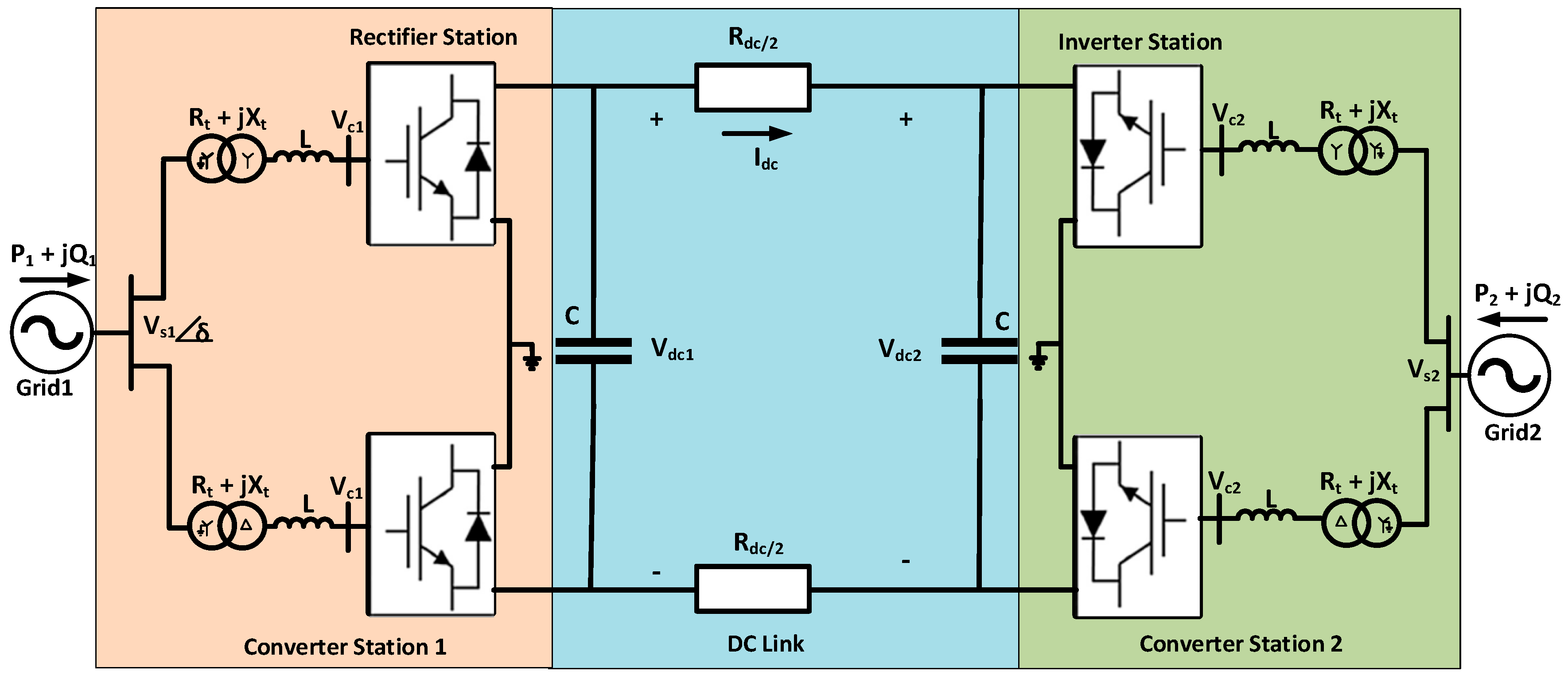
A detailed bidirectional VSC-based HVDC light system configuration is shown in Figure 1. It consists of two AC grids, two converter stations, and a DC link. Each converter station comprises of two poles, one with positive polarity and one with negative polarity, each with their neutral grounded. The converter stations are connected on one side to the AC network by transformers and grid filters and on the other side with the DC link. The main job of the AC transformers is to change the level of AC voltage so that it is compatible with the DC link voltage in the converter station. The line reactors facilitate the exchange of power between the VSC and the AC system and also help in attenuating the high frequency harmonics in the currents. The capacitors on the DC side of the converter provide voltage support and suppress the harmonics. In steady-state, no current flows through the grounded return, ensuring no corrosion of the ground conductors. In the event of a fault on one of the two poles, the system can still be operated as a monopolar HVDC with ground return. The total power that can be transferred with monopolar configuration is half that of bipolar configuration. The HVDC system in Figure 1 has the capability of bidirectional power flow. When the power flow is from gird-1 (grid-2) to grid-2 (grid-1), the conv-1 (conv-2) acts as AC to DC converter and conv-2 (conv-1) acts as DC to AC converter.

For analysis purposes, power flow from grid-1 to grid-2 is assumed. In Figure 1, the voltage $V_{s1}$ is the fundamental component of the voltage on the AC bus of grid-1, $V_{c1}$ is the fundamental component of the AC phase voltage at the converter input terminals at the rectifier station, and ${\delta }_1$ is the phase angle between the $V_{s1}$ and $V_{c1}$. Neglecting the resistance and harmonic components, the active and reactive power absorbed by the converter are given by (1) and (2),

$$P_{C1}=\frac{V_{s1}{V}_{c1}}{X_1}sin{\delta }_1$$

(1)

$$Q_{C1}=\frac{V_{s1}\left(V_{s1}-V_{c1}\cos {\delta }_1\right)}{X_1}$$

(2)

where $X_1$ is the total reactance between the AC source bus and the AC terminals of the converter, ignoring the resistance.

The implemented PWM technique has a DC voltage utilization ratio of 1 and modulation index m, and under linear modulation region we have,

$$V_{c1}=\frac{m}{\sqrt{2}}{V}_{dc1}$$

(3)

It is evident from (1)–(3) that active power flow and reactive power flow between the AC grid and converter station mainly depend on the phase angle $\delta$ and modulation index m. Hence, the active and the reactive power can be controlled by controlling $\delta$ and $m$, respectively. A similar expression can be obtained for $P_{C2}$ and $Q_{C2}$ by replacing the subscript 1 by 2 in (1)–(3). The control schemes at the rectifier and inverter stations are described below:

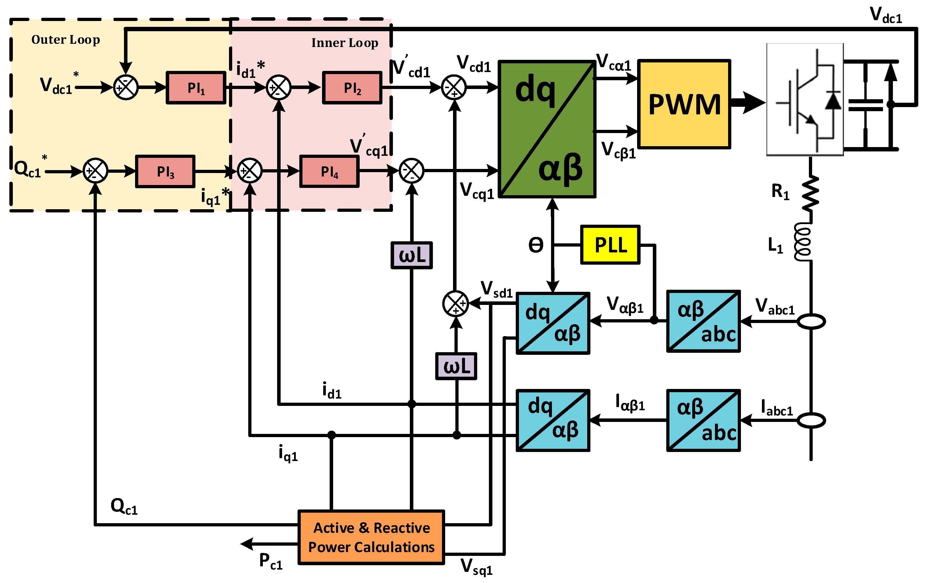
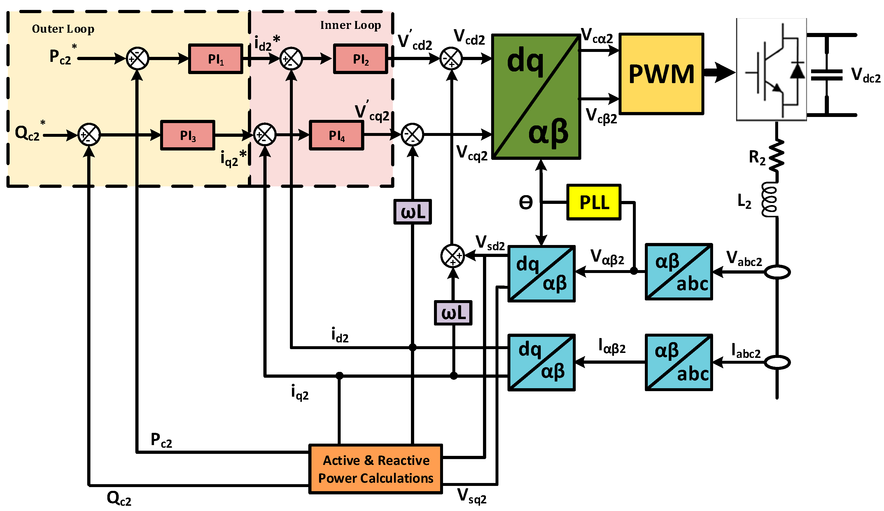
The block diagrams for the control mechanism at the rectifier station and inverter station are shown in Figure 2 and Figure 3 [10]. The control scheme consists of two loops, the inner loop controls the d-q components of current and an outer loop. The outer loop controls the DC link voltage $V_{dc1}$ and reactive power $Q_{c1}$ of the load connected to the rectifier side, whereas at the inverter station, the outer loop is used to control active power $P_{c2}$ and reactive power $Q_{c2}$.

3. Mathematical Model of VSC-Based HVDC Light System in d-q Reference Frame

The VSC-based HVDC light system shown in Figure 1, consists of three-phase, three-level, six pulse bridge converters at both rectifier and inverter stations. The converters are equipped with self-commutating insulated gate bi-polar transistor (IGBT) switches with antiparallel diodes. A detailed system configuration is given in Figure 1 and its parameters are given in

Table 1. Bidirectional VSC-based HVDC light system parameters.

Parameter	Symbol	Value
System rating	S	50 MVA
System frequency	f	50 Hz
Grid voltage	Vs	110 kv
Transformer low voltage	Vc	33 kv
Transformer reactance	Xt	9%
Transformer X/R ratio	Xt/Rt	6.63
Grid filter	L	15 mH
DC-link voltage	Vdc	±200 kV
DC capacitor	Cdc	200 µF
DC line resistance	Rdc	0.1 Ω/km (100 km)
Switching frequency	fsw	2850 Hz

Subscript 1 refers to converter 1 (rectifier) and subscript 2 refers to converter 2 (inverter).

. Each converter station is tied to the grid with equivalent impedances $Z_1=R_1+j\omega L_1$ and $Z_2=R_2+j\omega L_2$. It is assumed that converters are connected to strong AC grids.

The VSC-based HVDC light system model is given by the following set of differential equations in the d-q synchronous reference frame [9].

Rectifier Station:

$$\left[\begin{array}{c}{V}_{sd1}\\ V_{sq1}\end{array}\right]=R_1\left[\begin{array}{c}{i}_{d1}\\ i_{q1}\end{array}\right]+L_1\frac{d}{dt}\left[\begin{array}{c}{i}_{d1}\\ i_{q1}\end{array}\right]+\omega L_1\left[\begin{array}{c}-i_{q1}\\ i_{d1}\end{array}\right]+\left[\begin{array}{c}{V}_{cd1}\\ V_{cq1}\end{array}\right]$$

(4)

Inverter Station:

$$\left[\begin{array}{c}{V}_{sd2}\\ V_{sq2}\end{array}\right]=R_2\left[\begin{array}{c}{i}_{d2}\\ i_{q2}\end{array}\right]+L_2\frac{d}{dt}\left[\begin{array}{c}{i}_{d2}\\ i_{q2}\end{array}\right]+\omega L_2\left[\begin{array}{c}-i_{q2}\\ i_{d2}\end{array}\right]+\left[\begin{array}{c}{V}_{cd2}\\ V_{cq2}\end{array}\right]$$

(5)

In the synchronous reference frame, $v_{s1d},v_{s1q},v_{s2d},v_{s2q},i_{s1d},i_{s1q},i_{s2d}$, and $i_{s2q}$ are d and q axes components of instantaneous source voltages and currents, $v_{c1d},v_{c1q},v_{c2d}$, and $v_{c2q}$ are converter voltages along the d and q axes; ω is the angular frequency of the AC grid, $R_1$ and $R_2$ represent the total line resistance, and $L_1$ and $L_2$ represent the total line inductance from converter to AC grid. $P_1,P_2,Q_1$, and $Q_2$ are the active and reactive powers flowing from the AC grid to the converter stations, $V_{DC1}$ and $V_{DC2}$ are the DC bus voltages, and $I_{DC}$ is the DC link current. In (4) and (5), the d and q terms of the current are coupled in term 3 on right hand side, these can be decoupled by feedforward technique as shown in Figure 2 and Figure 3. The resulting equations are,

$$\left[\begin{array}{c}{V}_{xd1}\\ V_{xq1}\end{array}\right]=R_1\left[\begin{array}{c}{i}_{d1}\\ i_{q1}\end{array}\right]+L_1\frac{d}{dt}\left[\begin{array}{c}{i}_{d1}\\ i_{q1}\end{array}\right]$$

(6)

where, $\left[\begin{array}{c}{V}_{xd1}\\ V_{xq1}\end{array}\right]=\left[\begin{array}{c}{V}_{sd1}\\ V_{sq1}\end{array}\right]-\omega L_1\left[\begin{array}{c}-i_{q1}\\ i_{d1}\end{array}\right]-\left[\begin{array}{c}{V}_{cd1}\\ V_{cq1}\end{array}\right]$

$$\left[\begin{array}{c}{V}_{xd2}\\ V_{xq2}\end{array}\right]=R_2\left[\begin{array}{c}{i}_{d2}\\ i_{q2}\end{array}\right]+L_2\frac{d}{dt}\left[\begin{array}{c}{i}_{d2}\\ i_{q2}\end{array}\right]$$

(7)

where, $\left[\begin{array}{c}{V}_{xd2}\\ V_{xq2}\end{array}\right]=\left[\begin{array}{c}{V}_{sd2}\\ V_{sq2}\end{array}\right]-\omega L_2\left[\begin{array}{c}-i_{q2}\\ i_{d2}\end{array}\right]-\left[\begin{array}{c}{V}_{cd2}\\ V_{cq2}\end{array}\right]$.

The dynamic equations in (6) and (7) are first order systems and can be compensated using PI controllers as shown in Figure 2 and Figure 3, respectively.

Aligning the d-axis of the reference frame with the voltage at the AC grid results in constant d-axis and zero q-axis voltage components. Therefore, (8) and (9) give the instantaneous ac active and reactive powers, respectively,

$$P_{C1}=\frac{3}{2}\left(V_{sd1}{i}_{d1}+V_{sq1}{i}_{q1}\right)=\frac{3}{2}{V}_{sd1}{i}_{d1}$$

(8)

$$Q_{C1}=\frac{3}{2}\left(V_{sq1}{i}_{d1}-V_{sd1}{i}_{q1}\right)=-\frac{3}{2}{V}_{sd1}{i}_{q1}$$

(9)

The two converter stations are connected via a DC link. The DC power balance equation for the DC link is given by:

$$P_{dc1}=V_{dc1}{i}_{dc}=V_{dc2}{i}_{dc}+2R_{dc}{i}_{dc}^2$$

(10)

Assuming no power loss at the converter stations, the AC power is equal to the DC power as given by (11)

$$P_{ac1}=P_{dc1}=\frac{3}{2}{V}_{sd1}{i}_{d1}=V_{dc1}{i}_{dc1}$$

(11)

The dynamics of the $v_{dc1}$ are given by (12)

$$i_{dc1}=C\frac{d{v}_{dc1}}{dt}+\frac{v_{dc1}}{R_{load}}$$

(12)

where $R_{load}$ is Thevenin equivalent resistance seen form the DC terminals of the recitifier and C is the DC link capacitance.

Substituting (11) in (12), the DC link voltage v_dc1, can be written in terms of $i_{d1}$ as in (13)

$$\frac{3}{2}\frac{V_{sd1}}{V_{dc1}}{i}_{d1}=C\frac{d{v}_{dc1}}{dt}+\frac{v_{dc1}}{R_{load}}$$

(13)

Equation (13) represents a first order sytem, which can be compensated using a PI controller. Figure 2 and Figure 3 show the PI control schemes for rectifier and inverter stations, respectively. The $V_{q1}$ dynamics are related to $i_{q1}$ as in (9), and a PI controller is used to achieve zero steady state error. Similarly, $P_{c2}$ and $Q_{c2}$ dynamics can be related to $i_{d2}$ and $i_{q2}$ as in (8) and (9) respectively by replacing the subscript 1 by 2 and PI controllers are used to achieve zero steady state error. One converter has 4 PI controllers and therefore a total of 16 PI controllers are needed for a typical bidirectional HVDC light sytem shown in Figure 1.

4. Controller Tuning

The decoupled d-q axis control theory is employed in this paper to design controllers for the VSC converter stations. The control scheme consists of a nested control loop, the inner loop generates the d-q axes currents, and the outer loop control objective depends on the control mode of the VSC converter station. A VSC converter station can operate in the following control modes:

• DC voltage control
• Active power control
• Reactive power control

In this study, the rectifier station operates in modes a and c, whereas inverter station operates in modes b and c. The control schemes for rectifier and inverter stations are shown in Figure 2 and Figure 3, respectively. As evident from Figure 2 and Figure 3, each converter station requires four PI controllers to be tuned, and if the system parameters are different for two converters then the tuning procedure has to be repeated for each converter station. Tuning these many PI parameters by conventional methods is a cumbersome task, and moreover, the major challenge in such design methods is choosing appropriate bandwidths for inner and outer loops, which heavily depends on the designer’s experience. Hence, the tuned parameters using conventional methods do not exhibit optimal performance.

This paper proposes an innovative approach to design PI controllers for VSC-based HVDC light system. The idea is to automate the design process by introducing an optimization technique in the design procedure. Particle swarm optimization (PSO) is chosen as the optimization algorithm, owing to its simplicity in programming and fast convergence. Time-domain objective functions are optimized by the PSO. The following sections describe the PSO and the time-domain optimization of PI controllers.

4.1. Particle Swarm Optimization (PSO)

The PSO is an optimization algorithm based on social behavior and was inspired by a swarm of birds flying in unison without colliding with each other and moving towards their goal by sharing experiences of individuals and their colleagues in the swarm. PSO is a stochastic optimization algorithm and was developed by Eberhart and Kennedy. Similar to other evolutionary algorithms like the genetic algorithm (GA), PSO is a population-based optimization technique. The population is a collection of a predecided number of particles. Each particle in the population is a possible solution to the problem. The particles move around in the search space with dynamically changing velocity until its position ceases to change or until a stopping criterion is satisfied. During the flight, each particle flies around in the search space according to the historical experience of its own and the experience of its neighboring particles. The distinction of PSO over other heuristic algorithms based on evolution is that it has memory, i.e., every candidate solution (X) remembers its best solution, called local best( $J_{pbest}$), as well as the group best solution, called the global best( $J_{gbest}$). The other advantages of the PSO algorithm are it is simple to program, fast in convergence, and easy to implement [12].

In PSO, each particle keeps track of its own position and also the position of its neighbor. The best position achieved by each particle in the course of its flight is called $X_{pbest}$, and the corresponding solution is symbolized by $J_{pbest}$. At the beginning of the search, the global best denoted by $J_{gbest}$ is set to $J_{pbest}$ and the particle associated with it is denoted by $X_{gbest}$. As the search progresses, the particles are updated. Every particle updates itself through the above mentioned best positions. The individual particles update their own velocity (U_i) and their position according to the following equations [12,13],

$$U_i=F{U}_i+K_1{rand}_1()\left(X_{pbest}-X_i\right)+K_2{rand}_2()\left(X_{gbest}-X_i\right)$$

(14)

$$X=X_i+U_i$$

(15)

where $K_1$ and $K_2$ are cognitive and social constants, rand₁( ) and rand₂( ) are two random numbers between [0, 1], and $F$ is the inertia weight. $U_i$ denotes the velocity of ith particle, and $X_i$ denotes the corresponding particle position.

PSO Algorithm

The steps of the PSO algorithm used in this paper are described below:

i

A population of $n$ particles with random positions are initialized within the minimum and maximum bounds of the solution space. Similarly, $n$ corresponding velocities for the particles are initialized randomly. Fitness functions, $J$ are evaluated for the initial population

ii

Find the local best solution ($J_{pbest}$) for the initial population and let the particle associated with it be called $X_p$ and global best solution ($J_{gbest}$) is set equal to local best solution ($J_{pbest}$).

iii

Update the weight $F$ using the following equation, where ‘$i\_max$’ is the maximum number of iteration.

$$F=F_{max}-\left(\frac{F_{max}-F_{min}}{i\_max}\right)i,$$

(16)

iv

Update the velocity ($U)$ of each particle using (14) and check whether the updated velocity ($U)$ is within the bounds [$U_{max}$, $U_{min}$]. If not, set it to the limiting values.

v

The position of each particle is updated using (15), which forms the new population and repeat step iv for the new population.

vi

Calculate the fitness functions $J$ for the new population.

vii

Find the particle’s best solution ($J_{pbest}$) for fitness functions $J$ in the previous step.

viii

Compare the new best solution of the particle ($J_{pbest}$) with the global best solution( $J_{gbest}$). If $J_{pbest}$ is better than $J_{gbest}$ then set $J_{gbest}$ to $J_{pbest}$.

ix

The algorithm stops if stopping criteria are met, otherwise the procedure is repeated from step v. The stopping criteria are attaining the maximum number of iterations or the fitness value is not changing for a predetermined number of times.

4.2. Time-Domain Optimization of PI controllers

Voltage oriented control (VOC) topology based on the decoupled d-q axes theory using linear PI controllers is employed in this research. The advantage of this approach is that it allows independent control of active and reactive power [9]. Tuning rules for the PI controllers are well documented in the literature, and the conventional tuning methods for PI controllers rely on root locus and bode plots. Pole placement and pole-zero cancellation are some of the techniques that are used to select the parameters of the PI controllers for linearized first-order models of the VSC converters. One of the major drawbacks of these conventional techniques is that they only ensure the stability of the system without giving much emphasis to system performances like the overshoot, settling time, steady-state error, etc. Moreover, the design procedure in the conventional method heavily depends on the linearized model of the VSC converter. Furthermore, the design of PI controllers for the VSC-based HVDC light system is cumbersome if the system parameters for the two converters are different. In this paper, the selection of PI parameters for the VSC converters is automated by embedding an optimization algorithm in the design steps. Particle swarm optimization (PSO) is chosen because of ease in programming and fast in convergence. The design procedure is employed directly on the Simulink model of the bidirectional HVDC light system, which includes both converters and the complex power system along with the HVDC link. PSO can be chosen to minimize the following time-domain performance indices: integral absolute error (IAE) ($J={\int }_0^{\infty }\left|e\right|$), integral time absolute error (ITAE) ($J={\int }_0^{\infty }\left|te\right|$), integral square error (ISE) ($J={\int }_0^{\infty }\left|e^2\right|$), and integral time square error (ISE) ($J={\int }_0^{\infty }\left|t{e}^2\right|$). In this paper, the second performance index (ITAE) is optimized by the PSO algorithm to obtain the parameters of the inner and outer loop PI controllers shown in Figure 2 and Figure 3, though other performance indices can also be used to tune the PI controllers.

4.3. Controller Tuning by Conventional Modulus Optimum Method

Modulus optimum (MO) method is the conventional optimization method that is widely used to tune the PI control loops for grid-connected voltage source converters [19,20]. The important thing to consider when designing PI controllers using the MO method is to ensure that the magnitude of the closed-loop transfer function is kept close to unity or 0 dB over a large range of frequencies. The MO method is used when a system has one large time constant and several small-time constants. These small-time constants can be added to obtain an equivalent time constant. The details of tuning the PI controllers for grid-connected are given in [19,20]. The design procedure is briefly discussed as follows; if the transfer function of a system consists of one large time constant, T_L, and three small time constants $T_1,T_2$, and $T_3$, the open-loop transfer function can be written as in (13)

$$G_{ol}=\frac{K}{\left(1+T_L\right)\left(1+T_1\right)\left(1+T_2\right)\left(1+T_3\right)}$$

(17)

where $K$ is the system gain. The small time constants can be combined into one equivalent time constant as in (14)

$$T_{eq}=T_1+T_2+T_3$$

(18)

Then (18) can be written in a simplified form as in (19)

$$G_{ol}=\frac{K}{\left(1+T_L\right)\left(1+T_{eq}\right)}$$

(19)

The open-loop transfer function in cascade with the PI controller can be written as in (20)

$$G_{ol}=K_p\left(\frac{1+s{T}_i}{s{T}_i}\right)\frac{K}{\left(1+T_L\right)\left(1+T_{eq}\right)}$$

(20)

where $K_p$ and $T_i$ are proportional gain and integral time constant, respectively. $K_i$ can be obtained from $T_i$ as $K_i=\frac{K_p}{T_i}$.

Using MO method and on applying the pole-zero cancellation of the dominating pole of the system and optimizing the absolute value for the closed-loop system with the PI controller to unity, the PI parameters than can be written as in (21)

$$K_p=\left(\frac{T_L}{2K{T}_{eq}}\right)and{T}_i=T_L$$

(21)

The MO algorithm discussed above is applied for the system shown in Figure 1. From (6) and (7), the simplified first order inner current loop transfer function of the rectifier station (conv-1) can be written as in (22)

$$G_{io1}\left(s\right)=\frac{i_{d1}\left(s\right)}{i_{d1}^{*}\left(s\right)}=\frac{i_{q1}\left(s\right)}{i_{q1}^{*}\left(s\right)}=\left(\frac{1}{s{L}_1+R_1}\right)\left(\frac{1}{s\frac{T_{sw}}{2}+1}\right)=\frac{K}{\left(1+T_L\right)\left(1+T_{eq}\right)}$$

(22)

where $T_{sw}$ is the switching time period. Now, from the MO method, the inner current loop PI controller parameters can be obtained from (17).

Similarly for the outer DC voltage loop, from (13), the simplified first order transfer function is as in (23)

$$G_{vo1}\left(s\right)=\frac{V_{dc1}\left(s\right)}{V_{dc1}^{*}\left(s\right)}=\left(\frac{R_{load}}{s(R_{load}C)+1}\right)$$

(23)

where R_load is Thevenin equivalent resistance seen from the DC terminals of the recitifier, and C is the DC link capacitance. Now, MO can be applied to get the outer loop PI control parameters. The values of the PI parameters for the rectifier station (conv-1) are given in

Table 2. PI parameters for rectifier station (Conv-1).

Parameter	PSO	MO
$K_{Pid1}=K_{Piq1}$	375.6885	25.3650
$K_{i_{d1}}=K_{iq1}$	115.2844	190.0
$K_{PVdc1}$	0.2034	0.015
$K_{iVdc1}$	67.2170	25.0

. A similar approach can be applied at the inverter station (conv-2) to obtain the PI parameters for con-2.

5. Results and Discussions

The proposed approach is implemented on the VSC-based HVDC light system shown in Figure 1. The PSO algorithm was used to minimize the time domain based performance indices as discussed in Section 4. The PSO parameters selected for the optimization process are given in

Table 3. Particle swarm optimization (PSO) parameters.

Parameter	Value
Max Iterations	100
Max Weight	0.90
Min Weight	0.40
Swarm Population Size	20
$K_1$	2
$K_2$	2

.

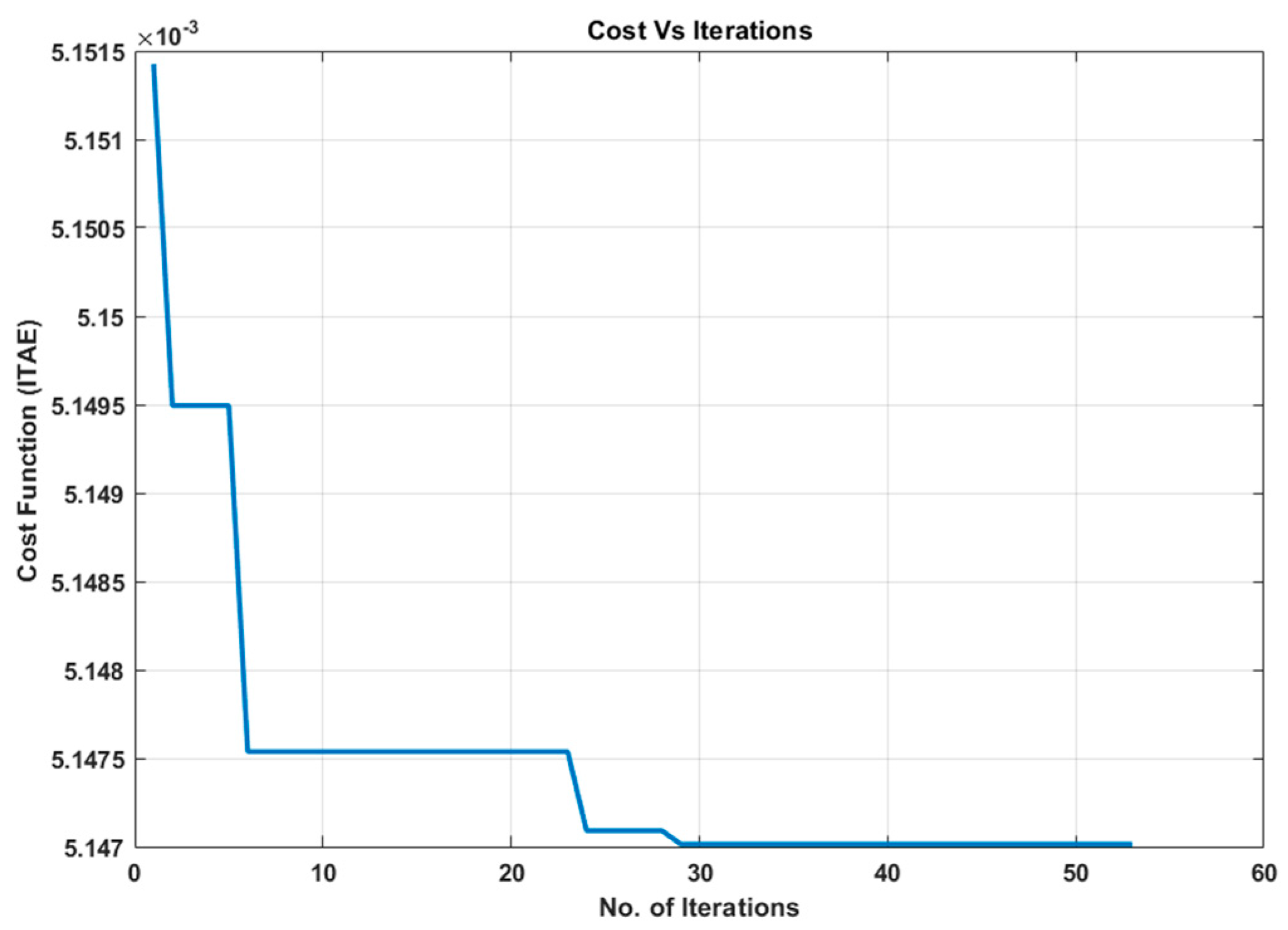
The proposed PSO-based tuning algorithm was implemented on a desktop computer with Intel Core i7 processor and a speed of 3.4 GHz. The size of the RAM was 12GB running on 64-bit Windows 10 operating system. The MATLAB version was 9.6 and Simulink version 9.3. It took about 4 hours for the PSO to optimize the PI parameters for the bidirectional HVDC. The convergence of the chosen cost function (ITAE) is shown in Figure 4. As seen in Figure 4, the PSO algorithm exited the optimization loop when the value of the cost function remains unchanged for 25 iterations.

The tuned PI parameters obtained by PSO and MO methods for the inner and outer loops are given in Table 2.

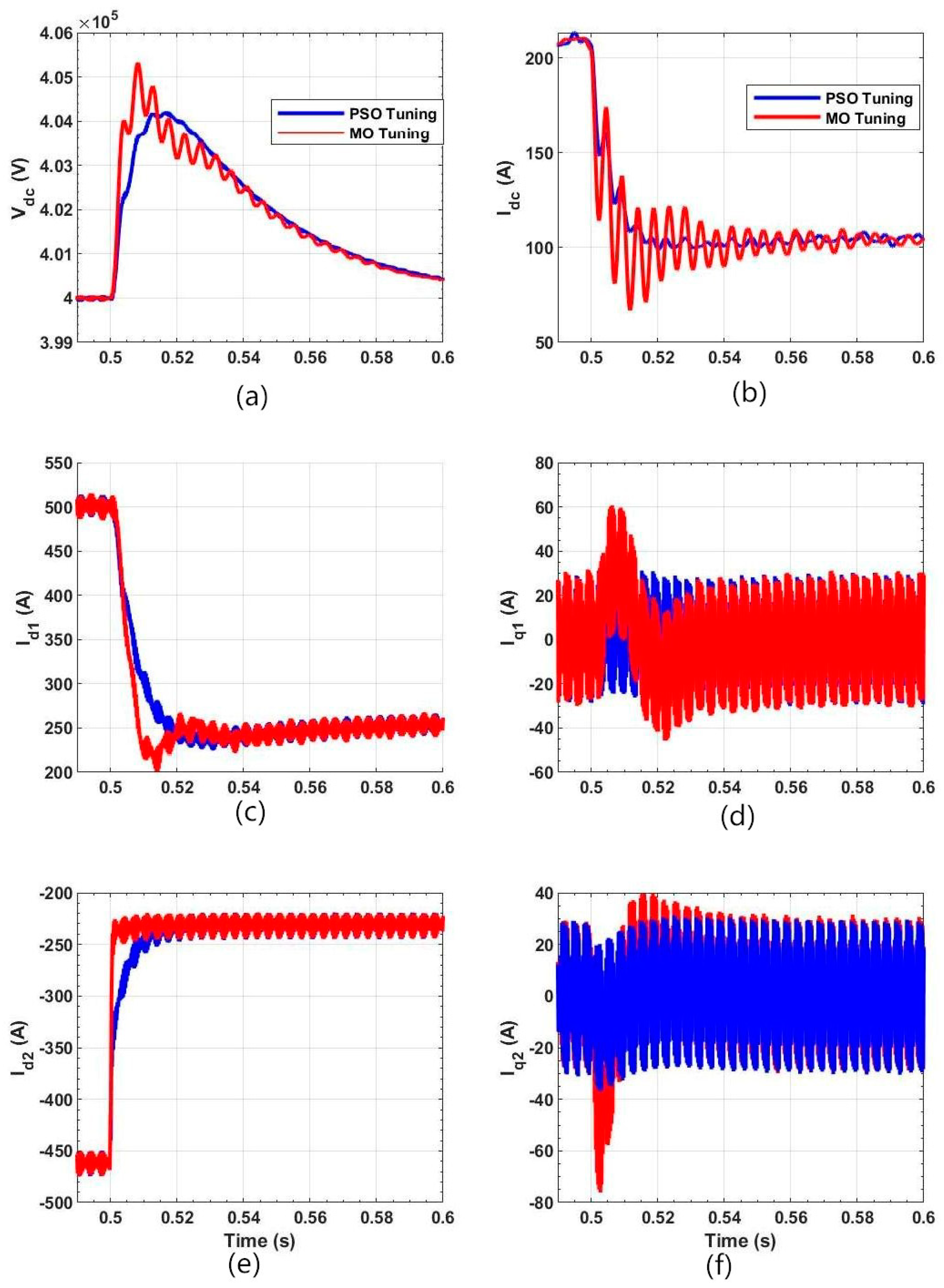
From Table 2 we can see that the parameters obtained from PSO are different from MO. These parameters are applied to the system in Figure 1 and the performance of the system is studied. The step response of the system for a step change in 50% of the load is studied and the results are given in Figure 5. Even though in the actual system such a large sudden change in load does not happen, in order to study the system behaviors a 50% step change is considered. Figure 5 shows the response of the $V_{dc1}$. The MO parameters give higher overshoot and oscillations, whereas PSO parameters result in optimal performance with desired setting time, overshoot, and no oscillations in steady state. The response of d and q components of AC side currents of rectifier and inverter respectively can also be seen in Figure 5. As expected, the PSO parameters give a better response compared to MO parameters. These components have higher oscillations when MO parameters are used. Figure 5 shows the response of d and q components of rectifier and inverter currents, respectively. As expected, the PSO parameters give a better response compared to MO parameters. These results show that the parameters obtained from the MO method are not optimal, and additional manual tuning is required to further improve the response.

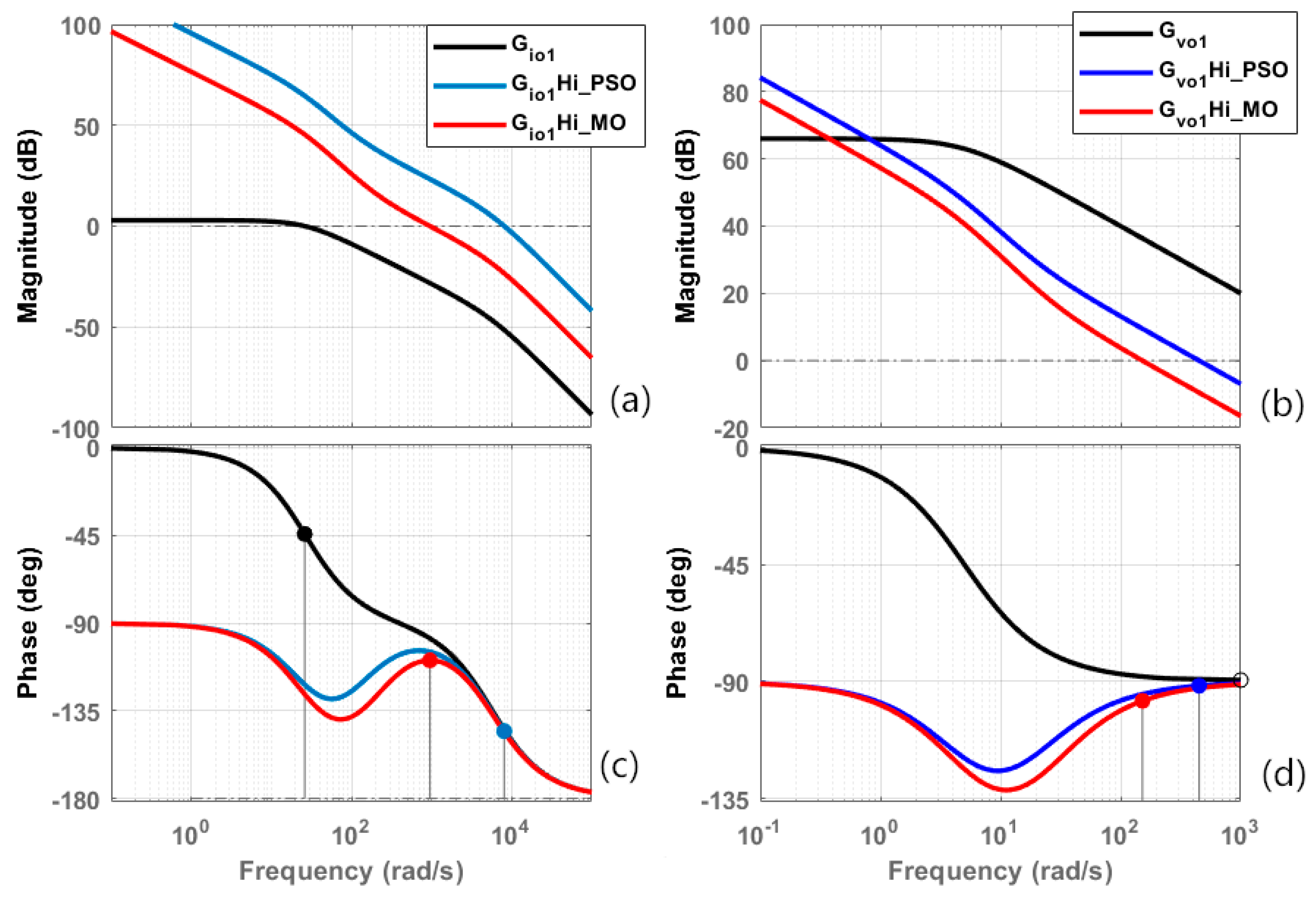
Figure 6 shows the bode plot of the inner current loop and outer DC voltage loop with PI, using parameters obtained from PSO and MO methods. The open loop bandwidth of the inner loop is 26 rad/s, phase margin of 136°, and the steady state gain is very low. The PI controller with parameters using MO improved the phase margin to 70°, steady state gain to 73 dB, and bandwidth to 1000 rad/s. The PI controller with parameters using PSO improved the phase margin to 34.5°, steady state gain to 98 dB, and bandwidth to 8000 rad/s. This clearly shows that the bandwidth obtained by the MO is not optimal and the PSO guarantees higher bandwidth, thus better utilization of system bandwidth. Similar observations can be made from the open loop bode plot of the outer DC voltage loop. The outer DC voltage loop has a very low DC gain, and the DC gain improvement for the PSO tuning method is better than the MO tuning method. Furthermore, the phase margin is better for the PSO tuning method compared to the MO.

In Figure 7, the behavior of the system when line-line-line to ground LLLG fault occurs on the AC side of the inverter section is studied. Under this condition, the AC voltage at the converter terminals is collapsed to zero and as per the grid operation standards [19,20], the DC bus needs to be maintained for two cycles of the input AC. Figure 7 shows the response of the $V_{dc1}$. Similar to previous results in Figure 5, the MO parameters give higher overshoot and oscillations, whereas PSO parameters result in optimal performance with desired setting time, overshoot, and no oscillations in steady-state. The result in Figure 7 shows that the PSO parameters give a better response compared to MO parameters as far as d and q components of currents are concerned. As expected, the PSO parameters give a better response compared to MO parameters. The d and q components of currents have more oscillations when MO parameters are used. These results show that the parameters obtained from the MO method are not optimal and additional manual tuning is required to further improve the response.

6. Conclusions

In this paper, an optimal tuning method using PSO to design PI controller parameters for the inner and outer control loops of a bidirectional HVDC light system is presented. The tuning of the PI controllers is achieved by embedding the PSO algorithm in the design steps directly on the Simulink model of the system. The Simulink model includes all the dynamics of the system and no simplifications are used. The results demonstrate the effectiveness of the design approach. The advantages of the design approach include the automation of the design procedure, which requires minimum input from the designer making the design independent of the designer’s experience. Additionally, in a system like a bidirectional HVDC light system, where a large number of PI controllers are to be tuned especially when the system parameters for the rectifier and inverter stations are different, automation of the design process is the way to go instead of repeating the design again and again manually. The proposed method is verified through simulation and simulation results are presented.