Design and Modeling of an Integrated Flywheel Magnetic Suspension for Kinetic Energy Storage Systems


Abstract
1. Introduction
- There are very limited winding losses because the steady-state suspension force is always applied by the PM flux;
- There are no flux variations in static conditions, resulting in negligible rotor losses and the possibility to adopt solid magnetic cores instead of laminated stacks;
- Possible eddy currents generated at dynamic condition provide a damping effect, improving the stability control;
- The flywheel itself provides a high surface available for the axial force application, without introducing additional rotating cores;
- There is independent control for the UCs and the LC;
- Simpler UCs control assessment as the force current characteristic is almost linear because of the DC bias due to the PM flux;
- There is an inherent self-centering effect in the radial direction, possibly controlled by both the coil currents.
2. System Description
- The rated air-gap length must be large enough to deal with high-rate disturbances, the compensation of which could require high electrical and thermal stresses to the AHMB coils;
- Temperature increase deteriorates the PM properties with possible loss of the stable condition;
- The lower the coercivity, the thicker the PM must be, therefore decreasing the useful steel surface; the consequent higher can be obtained only with higher PM and core volumes.
3. AHMB Electromagnetic Design
- (a)
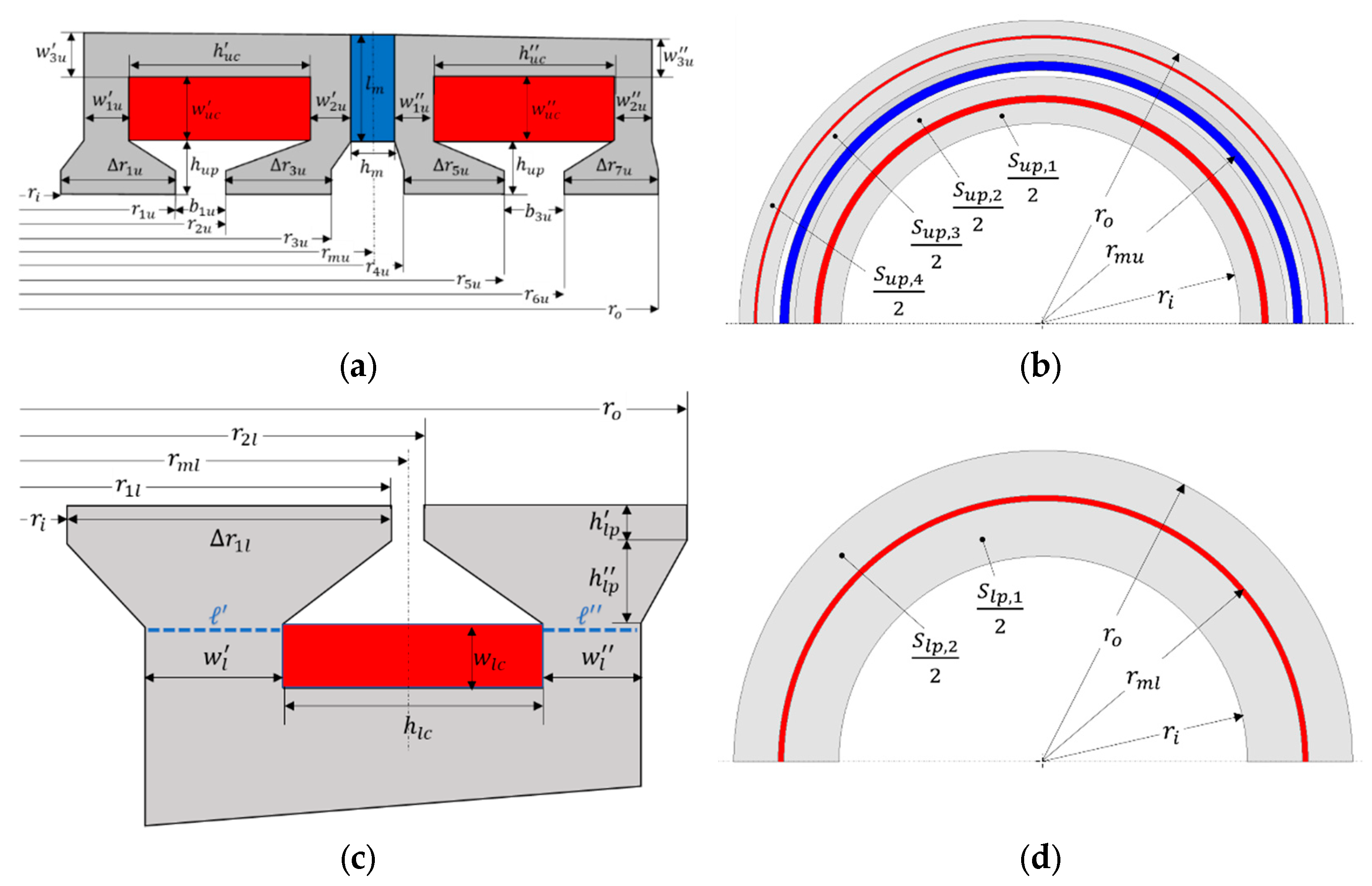
- radial bounds defined by and ;
- (b)
- equal annular cross section for all the pole shoes, that are (h = 1, …, 4) for the upper side and (j = 1, 2) for the lower side; such a condition should ensure uniform flux density distribution, resulting in evenly distributed axial force among the pole shoes on the same side;
- (c)
- equal height for all the pole shoes (upper side , lower side );
- (d)
- equal annular cross section of the core legs (h = 1, …, 4) for the upper side and (j = 1,2) for the lower side; and are decreasing factors to enable enough room for the coil placement; their choice must consider local magnetic saturation, even with the coil mmf contribution;
- (e)
- equal cross section of the upper coils considering that they should provide the same mmf with the same current density;
- (f)
- PM operation near the maximum energy point (little higher than ) at the rated air-gap length with unexcited coils;
- (g)
- fixed variation range for the PM height and radius for manufacturing and cost issues.
3.1. Upper Side
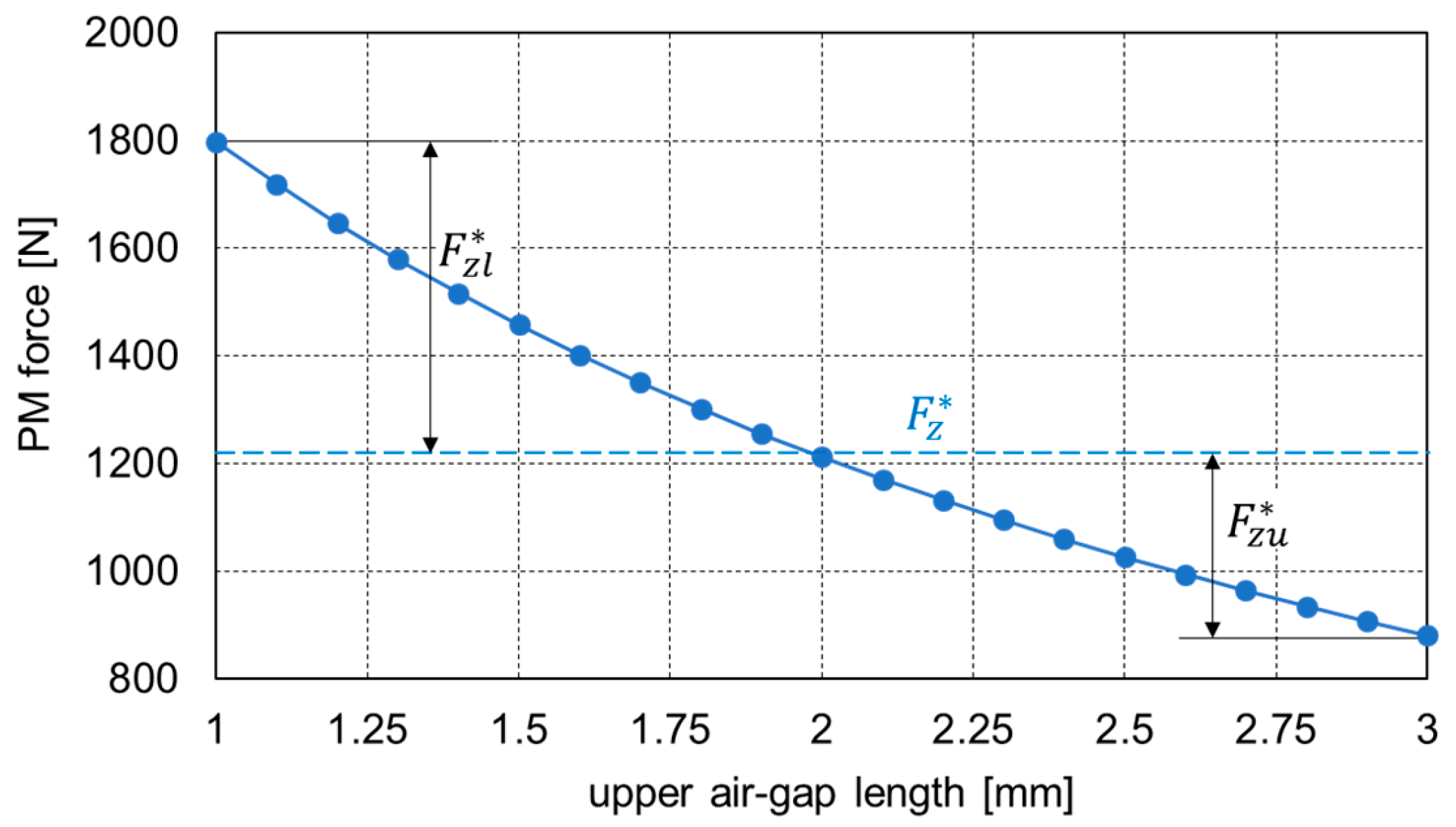
- the suspension force at the air-gap due to the only PM;
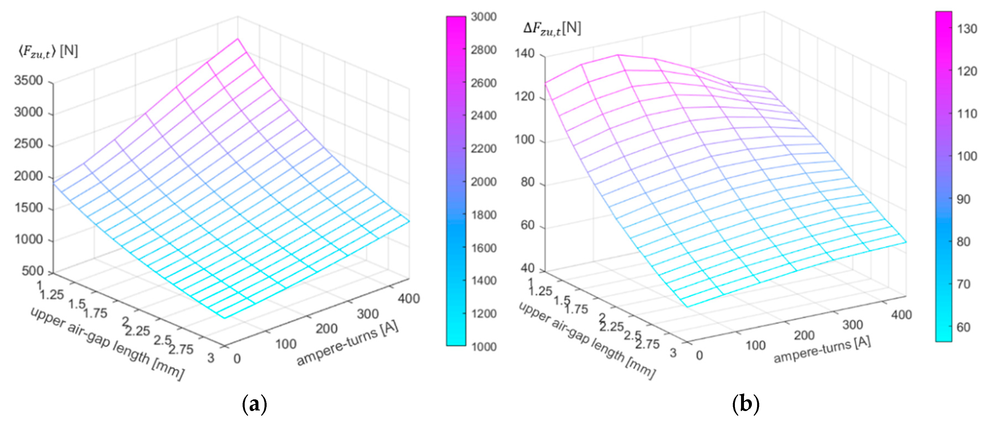
- the suspension forces and with augmented air-gap due to the PM only and in the presence of current excitation (current density ), respectively;
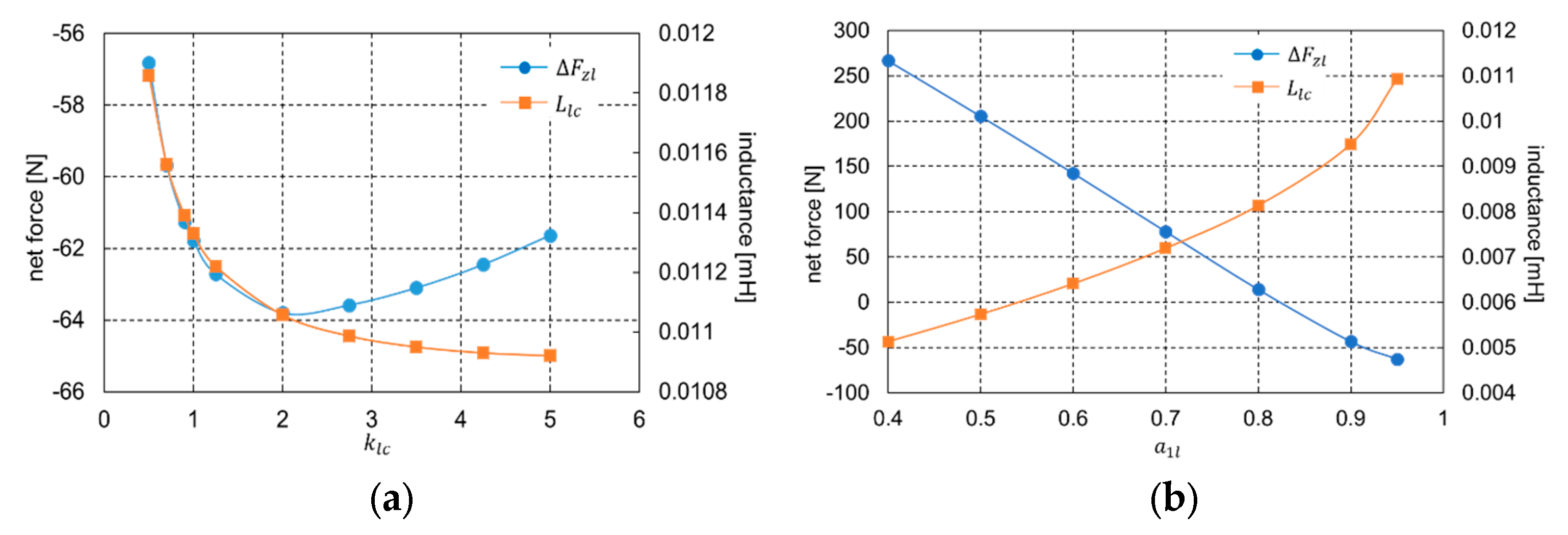
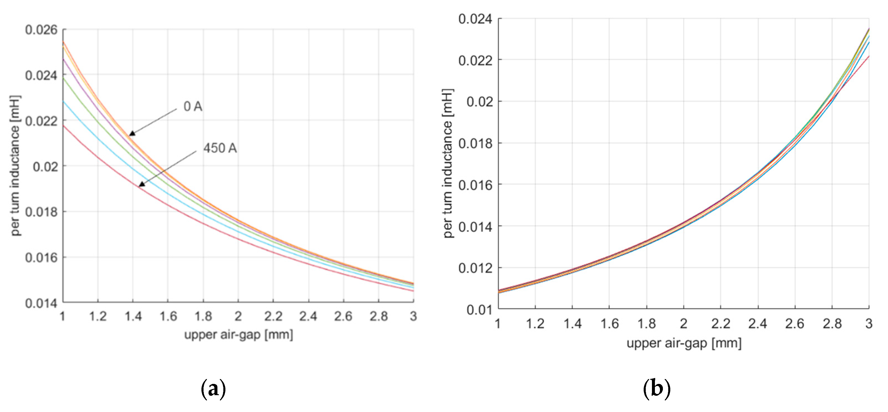
- the coil per-turn inductance in the same condition as is calculated; because of the series connection and the chosen current polarity, it is , with being the inner and outer coil inductances, respectively, and being the mutual inductance coefficient.
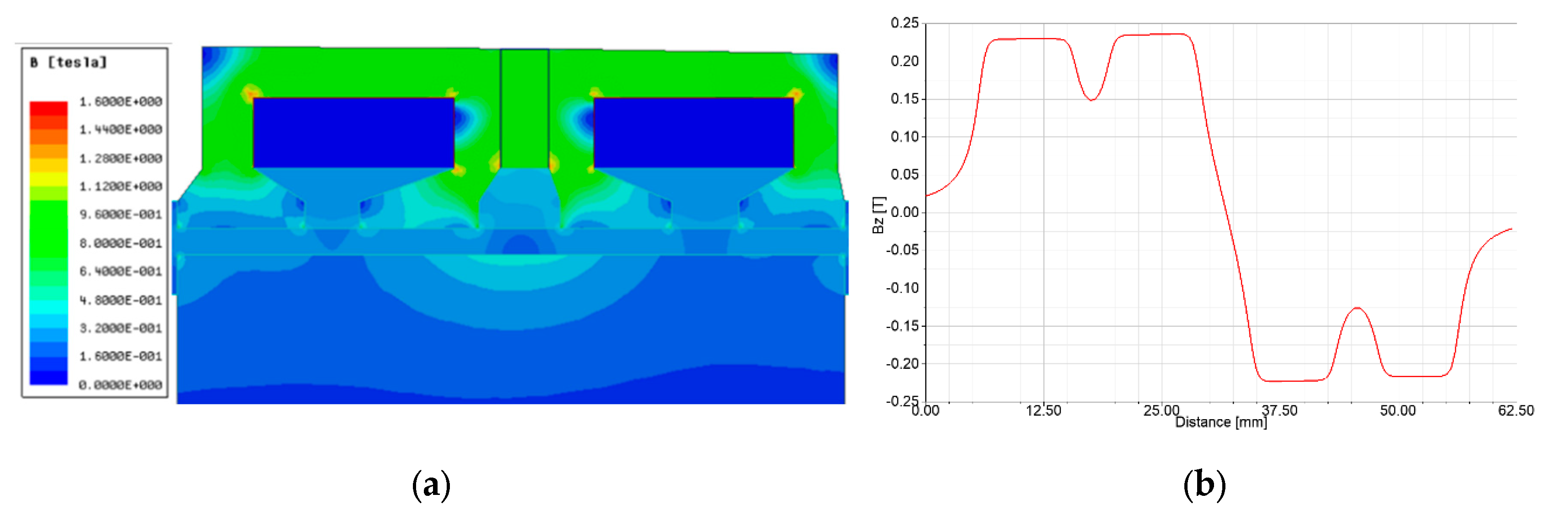
3.2. Lower side
- constant coil section with variable aspect ratio ; it follows that and ;
- variable pole shoe height + with fixed value for .
4. Control System
4.1. Model of the Suspension Dynamics
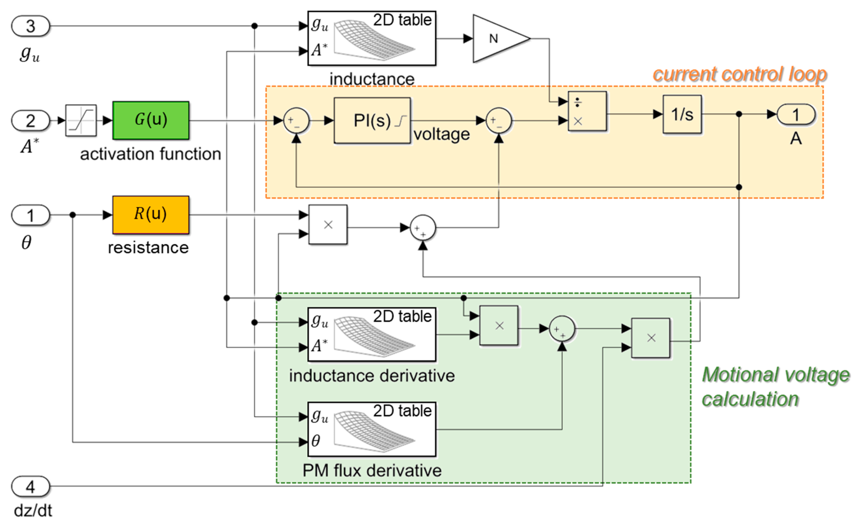
4.2. Electrical Model
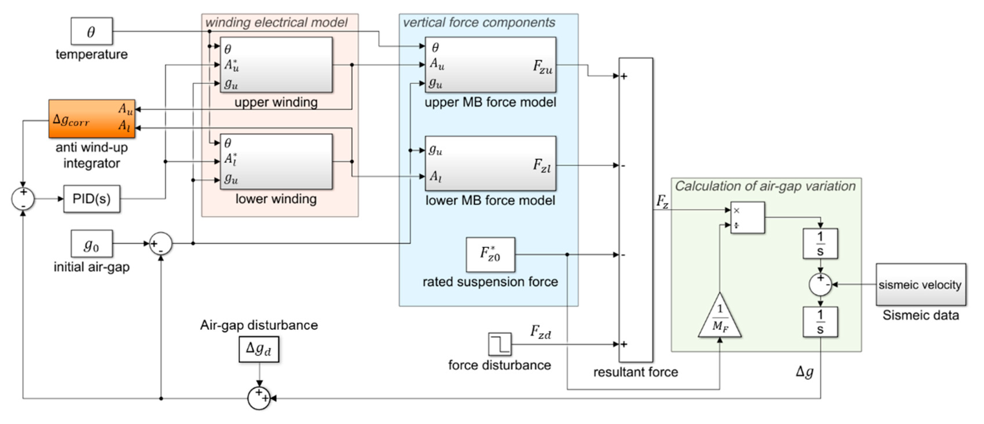
4.3. Overall Model
- an external force added to the force balance; in practical cases, such contribution can derive from vertical attraction forces between the rotor and the stator of the electrical machine;
- an air-gap variation caused, for instance, by a sudden motion of the AHMB fixed parts;
- a superimposed vertical velocity , simulating, for instance, the effect of an earthquake (instantaneous data of a seismic velocity).
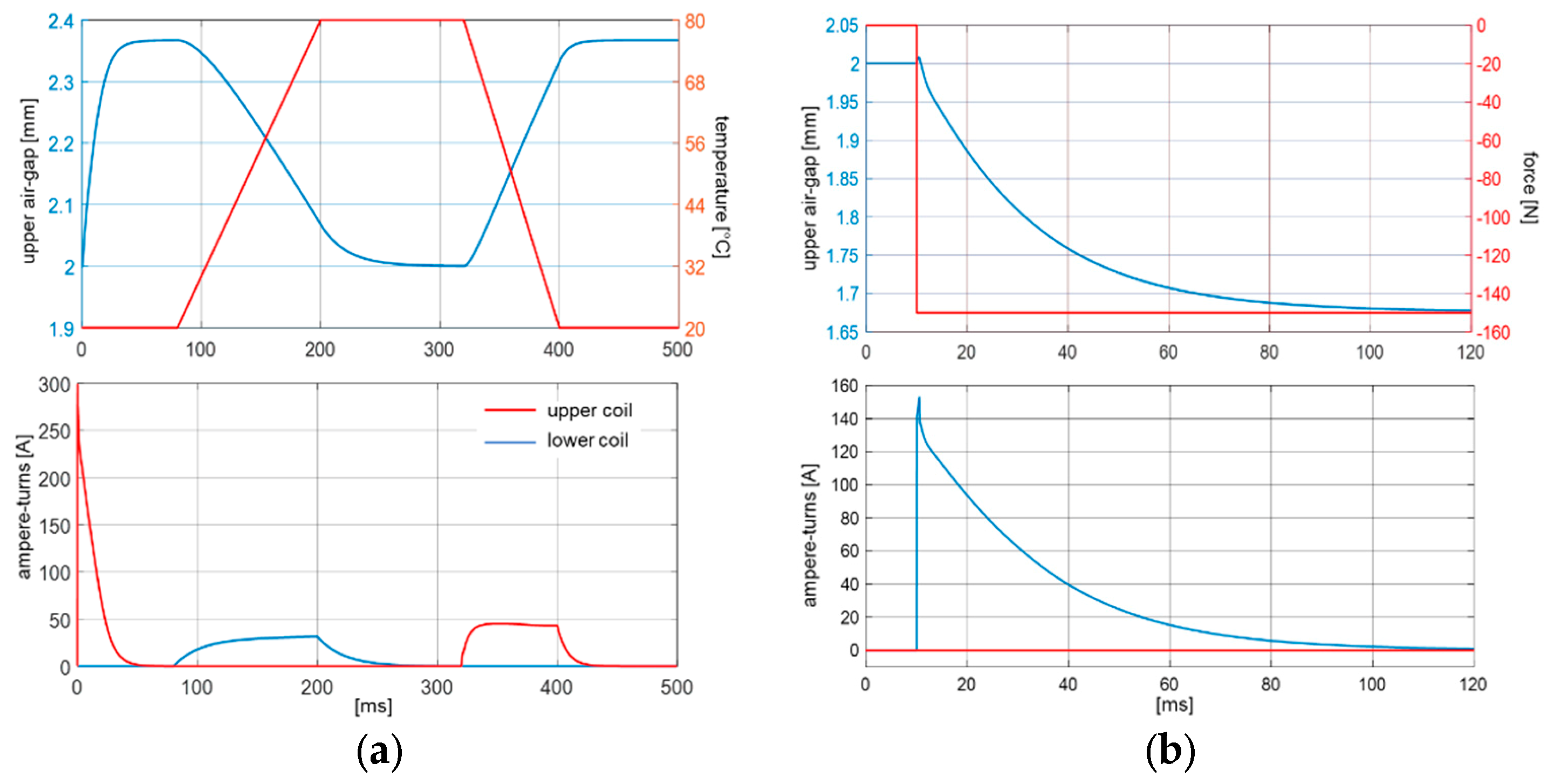
5. Simulation Results
6. Conclusions
Author Contributions
Funding
Conflicts of Interest
List of symbols
| weighting coefficients of the performance index P | |
| per-unit variables used for the parametrization of the upper pole shoes geometry | |
| per-unit variable used for the parametrization of the lower pole shoe geometry | |
| upper and lower coil ampere-turns | |
| slot openings of the upper cores | |
| PM remanence, coercivity, and temperature coefficient | |
| mean air-gap flux density (axial component) | |
| saturation flux density and magnetic permeability | |
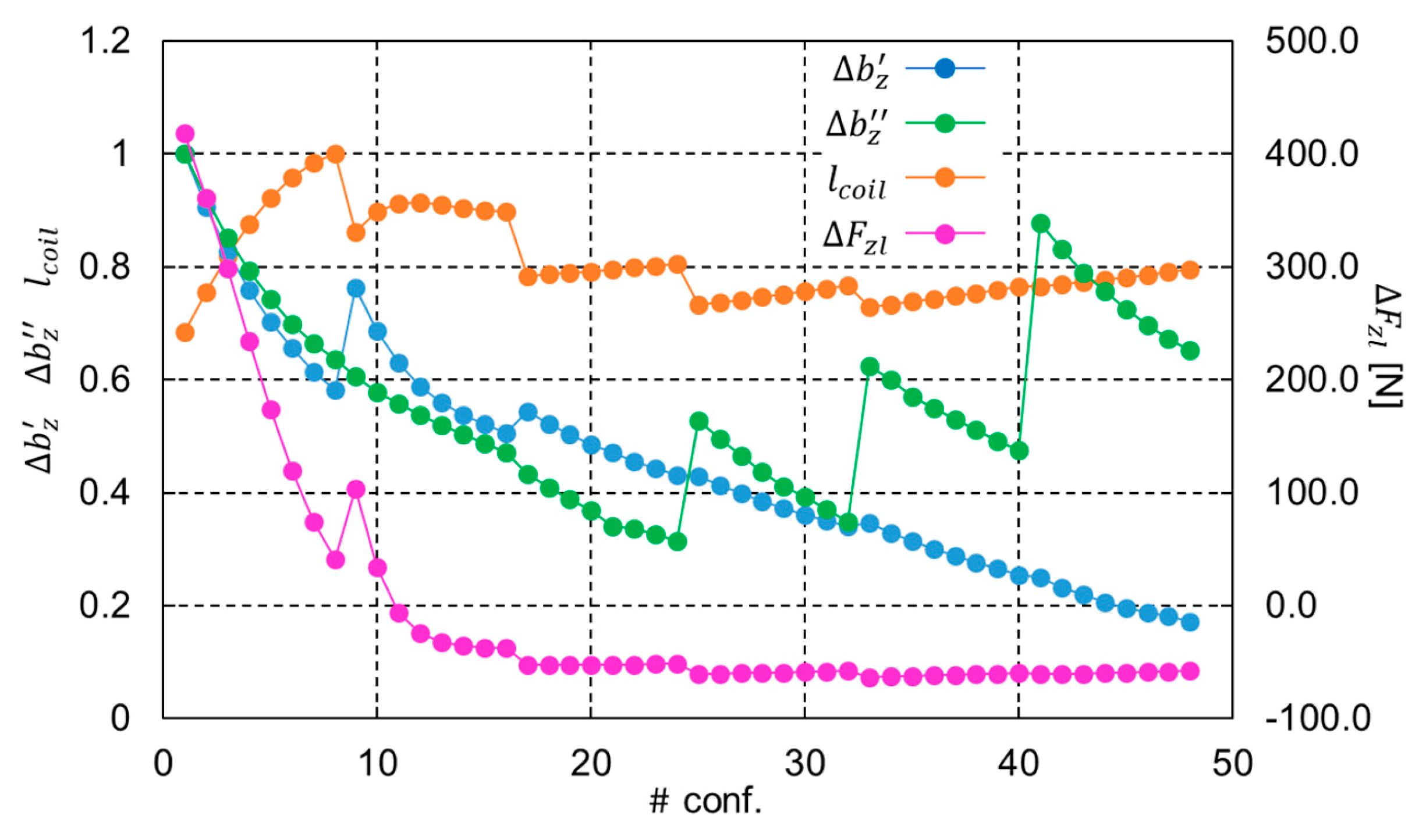
| , | standard deviations of the axial flux density in the lower core legs |
| net axial force with lower coil excitation | |
| air-gap deviation with respect to and its maximum value | |
| air-gap disturbance | |
| pole shoe widths of the inner and the outer cores (upper side) | |
| width of the inner pole shoe of the lower side core | |
| resultant, PM, upper side and lower side force contribution | |
| requested force for the total mass suspension | |
| rated value of the PM suspension force | |
| , | PM suspension forces at and ; |
| upper side suspension forces at with current excitation; | |
| PM force deviation at the maximum and minimum air-gap bounds; | |
| contributions of upper side force model dealing with temperature variation | |
| force and air-gap disturbances | |
| air-gap length at balanced condition with no coil supply | |
| upper and lower air-gap length | |
| height of the upper and lower pole shoes | |
| height and width of the inner coil (upper side) | |
| height and width of the outer coil (upper side) | |
| height and width of the lower coil | |
| PM height, length and volume | |
| flywheel shape factor, rated energy amount, and rotational inertia | |
| weighting coefficient to model the force with temperature variations | |
| coil filling factor, upper and lower coil cross sections | |
| per-turn inductance, resistance, and PM flux | |
| upper and lower coil inductance | |
| flywheel and additional masses | |
| maximum flywheel speed and speed ratio | |
| performance index | |
| operating temperature and temperature coil rise | |
| mass density, ultimate and low-cycle fatigue stresses | |
| , | copper resistivity at and thermal coefficient |
| upper and lower coil current density | |
| radial coordinates of the upper pole shoes | |
| radial coordinates of the lower pole shoes | |
| mean PM radius | |
| mean coil radius of the lower side coil | |
| outer and inner radius of the flywheel rotor rim | |
| mean coil radius of the upper side coils | |
| upper and lower coil ohmic resistance | |
| rim surface and surface utilization factor | |
| annular cross section of the k-th pole shoe (up: upper side, lp: lower side) | |
| annular cross section of the k-th core leg (ul: upper side, ll: lower side) | |
| supply voltage and coil turns | |
| , | maximum and minimum flywheel angular speed |
| width of the inner and of the outer core legs (upper side) | |
| width of the lower side core legs | |
| thickness of the inner and outer yokes (upper side) |
References
- Dambone Sessa, S.; Tortella, A.; Andriollo, M.; Benato, R. Li-Ion Battery-Flywheel Hybrid Storage System: Countering Battery Aging During a Grid Frequency Regulation Service. Appl. Sci. 2018, 8, 2330. [Google Scholar] [CrossRef]
- Lazarewicz, M.L.; Rojas, A. Grid frequency regulation by recycling electrical energy in flywheels. In Proceedings of the IEEE Power Engineering Society General Meeting, Denver, CO, USA, 6–10 June 2004. [Google Scholar]
- Rhode Hybrid Test Facility. Available online: http://schwungrad-energie.com/vs/2017/06/Schwungrad-Energie_EirGrid-Demonstration-Project-Report.pdf (accessed on 8 November 2019).
- Amiryar, M.E.; Pullen, K.R.; Nankoo, D. Development of a High-Fidelity Model for an Electrically Driven Energy Storage Flywheel Suitable for Small Scale Residential Applications. Appl. Sci. 2018, 8, 453. [Google Scholar] [CrossRef]
- Yulong, P.; Cavagnino, A.; Vaschetto, S.; Feng, C.; Tenconi, A. Flywheel Energy Storage Systems for Power Systems Application. In Proceedings of the 6th International Conference on Clean Electrical Power (ICCEP), Santa Margherita Ligure, Italy, 27–29 June 2017. [Google Scholar] [CrossRef]
- Amiryar, M.E.; Pullen, K.R. A Review of Flywheel Energy Storage System Technologies and Their Applications. Appl. Sci. 2017, 8, 286. [Google Scholar] [CrossRef]
- Schweitzer, G. Active magnetic bearings-chances and limitations. In Proceedings of the 6th International Conference on Rotor Dynamics, Sydney, Australia, 30 September–4 October 2002. [Google Scholar]
- Amrhein, W.; Silber, S. Magnetic Bearing Technology. In Magnetic Bearings; Schweitzer, G., Maslen, E.H., Eds.; Springer: Berlin/Heidelberg, Germany, 2009; pp. 417–447. [Google Scholar]
- Werfel, F.N.; Floegel-Delor, U.; Rothfeld, R.; Riedel, T.; Goebel, B.; Wippich, D.; Schirrmeister, P. Superconductor bearings, flywheels and transportation. Supercond. Sci. Technol. 2012, 25, 014007. [Google Scholar] [CrossRef]
- Zhang, W.; Zhu, H. Radial magnetic bearings: An overview. Results Phys. 2017, 7, 3756–3766. [Google Scholar] [CrossRef]
- Abrahamsson, J.; Bernhoff, H. Magnetic bearings in kinetic energy storage systems for vehicular applications. J. Electr. Syst. 2011, 7, 225–236. [Google Scholar]
- Liu, X.; Dong, J.; Du, Y.; Shi, K.; Mo, L. Design and Static Performance Analysis of a Novel Axial Hybrid Magnetic Bearing. IEEE Trans. Magn. 2014, 50, 1–4. [Google Scholar] [CrossRef]
- Bangcheng, H.; Bin, L. The Influences of Parameters on Performance of Hybrid Axial Magnetic Bearing. In Proceedings of the Intenational Symptom on Systems and Control in Aerospace and Astronautics, Shenzhen, China, 10–12 December 2008. [Google Scholar] [CrossRef]
- Toh, C.S.; Chen, S.L. Design, Modeling and Control of Magnetic Bearingsfor a Ring-Type Flywheel Energy Storage System. Energies 2016, 9, 1051. [Google Scholar] [CrossRef]
- Andriollo, M.; Scaldaferro, E.; Tortella, A. Design optimization of the magnetic suspension for a flywheel energy storage application. In Proceedings of the 2015 International Conference on Clean Electrical Power (ICCEP), Taormina, Italy, 16–18 June 2015. [Google Scholar] [CrossRef]
- Genta, G. Kinetic Energy Storage: Theory and Practice of Advanced Flywheel Systems, 3rd ed.; Butterworth & Co.: London, UK, 1985; pp. 80–87. [Google Scholar]
- Darrelmann, H. Comparison of High Power Short Time Flywheel Storage Systems. In Proceedings of the 21st International Telecommunications Energy Conf. (INTELEC ‘99), Copenhagen, Denmark, 9 June 1999. [Google Scholar] [CrossRef]
- Sokolov, A.; Jastrzebski, R.P.; Saarakkala, S.E.; Hinkkanen, M.; Mystkowski, A.; Pyrhonen, J.; Pyrhonen, O.A. Analytical method for design and thermal evaluation of a long-term flywheel energy storage system. In Proceedings of the 2016 International Conference on Power Electronics, Electrical Drives, Automation and Motion (SPEEDAM), Anacapri, Italy, 22–24 June 2016. [Google Scholar] [CrossRef]
- Chiba, A. Electro-magnetics and mathematical model of magnetic bearings. In Magnetic Bearings and Bearingless Drives; Newnes; Elsevier: Burlington, MA, USA, 2005; pp. 16–44. [Google Scholar]
- Itaca-ITalian ACcelerometric Archive. Available online: http://itaca.mi.ingv.it (accessed on 16 December 2019).


| FESS | Materials | |||
|---|---|---|---|---|
| Rated energy | 2.2 kWh | AISI 4340 | Ultimate strength | 1790 MPa |
| Maximum speed | 32000 rpm | Steel density | 7830 kg/m3 | |
| Speed ratio | 3 | Magnetic permeability | 600 | |
| Shape factor | 0.75 | Saturation flux density | 1.8 T | |
| Rotational inertia | 1.59 kg m2 | NdFeB | Remanence @20 °C | 1.1 T |
| Flywheel mass | 74 kg | Coercivity @20 °C | −838 kA/m | |
| Outer radius | 200 mm | Temperature coefficient | −0.12%/°C | |
| Inner radius | 132 mm | AISI 1008 | Maximum permeability | 1250 |
| Additional mass | 50 kg | Saturation flux density | 2.3 T | |
| Quantity | Value | Quantity | Value |
|---|---|---|---|
| Rated air-gap | 2 mm | Operating temperature | 80 °C |
| Maximum air-gap deviation | 1 mm | Coil filling factor | 0.6 |
| Average flux density | 0.24 T | Maximum core flux density | 1.8 T |
| Pole section | 131.4 mm2 | Core leg section | 263 mm2 |
| Maximum current density | 7 A/mm2 | Coil section | 110 mm2 |
| Pole shoe height | 4.5 mm | PM volume | 64 cm3 |
| PM thickness | 10 mm | PM height | 6 mm |
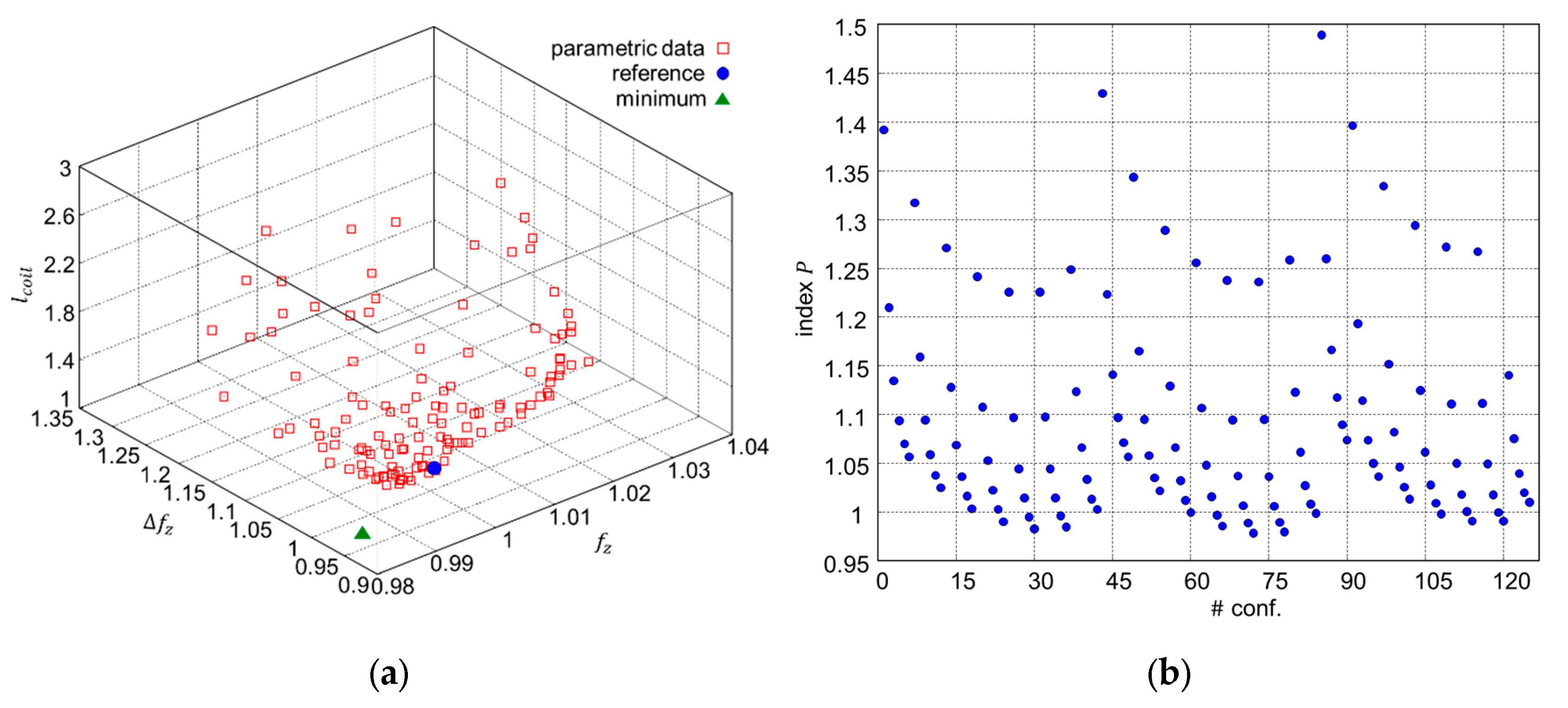
| Quantity | Reference Value | Optimal Value |
|---|---|---|
| [N] | 1210 | 1212 |
| [N] | 1211 | 1205 |
| 1.21 | 1.11 | |
| 1 | 0.979 | |
| [mm] | ||
| [mm] | ||
| [mm] | ||
| [mm] | ||
| [mm] | ||
| Quantity | Value | Quantity | Value |
|---|---|---|---|
| Coil section | 200 mm2 | Coil aspect ratio | 4.25 |
| Pole shoe height | 4 mm | Pole shoe width | 29 mm |
| Core leg reduction factor | 0.4 | Current density | 6.25 A/mm2 |
| Coil mean radius | 164 mm | Pole shoe tapered height | 8 mm |
| Standard deviation (inner leg) | 0.364 T | Coil per-turn inductance | 11.17 μH |
| Standard deviation (outer leg) | 0.249 T | Net axial force | −59.1 N |
| Parameters | Upper Side | Lower Side |
|---|---|---|
| Design current density | 4 A/mm2 | 6 A/mm2 |
| Winding design voltage | 60 V | 60 V |
| Maximum converter voltage | 200 V | 200 V |
| Turns/coil | 33 | 46 |
| Ohmic resistance @20 °C | 21.2 mΩ | 6.1 mΩ |
| Current regulator | ||
| Anti-windup constant | 10−4 | 5∙10−5 |
| Air-gap regulator | ||
| Temperature range | {20 °C, 80 °C} | |
© 2020 by the authors. Licensee MDPI, Basel, Switzerland. This article is an open access article distributed under the terms and conditions of the Creative Commons Attribution (CC BY) license (http://creativecommons.org/licenses/by/4.0/).
Share and Cite
Andriollo, M.; Benato, R.; Tortella, A. Design and Modeling of an Integrated Flywheel Magnetic Suspension for Kinetic Energy Storage Systems. Energies 2020, 13, 847. https://doi.org/10.3390/en13040847
Andriollo M, Benato R, Tortella A. Design and Modeling of an Integrated Flywheel Magnetic Suspension for Kinetic Energy Storage Systems. Energies. 2020; 13(4):847. https://doi.org/10.3390/en13040847
Chicago/Turabian StyleAndriollo, Mauro, Roberto Benato, and Andrea Tortella. 2020. "Design and Modeling of an Integrated Flywheel Magnetic Suspension for Kinetic Energy Storage Systems" Energies 13, no. 4: 847. https://doi.org/10.3390/en13040847
APA StyleAndriollo, M., Benato, R., & Tortella, A. (2020). Design and Modeling of an Integrated Flywheel Magnetic Suspension for Kinetic Energy Storage Systems. Energies, 13(4), 847. https://doi.org/10.3390/en13040847