Article

Lithium-Ion Battery SOH Estimation Based on XGBoost Algorithm with Accuracy Correction

Department of Electronic Engineering, Guangxi Normal University, Guilin 541004, China
*
Author to whom correspondence should be addressed.
Energies 2020, 13(4), 812; https://doi.org/10.3390/en13040812
Submission received: 5 January 2020 / Revised: 5 February 2020 / Accepted: 10 February 2020 / Published: 13 February 2020
(This article belongs to the Section F: Electrical Engineering)

Abstract

:
SOH (state of health) estimation is important for battery management. Since the electrochemical reaction inside LIBS (lithium-ion battery system) is extremely complex and the external working environment is uncertain, it is difficult to achieve accurate determination of SOH. To improve the accuracy of SOH estimation, we propose a SOH estimation method for lithium-ion battery based on XGBoost algorithm with accuracy correction. We extract several features, including average voltage, voltage difference, current difference, and temperature difference, to describe the aging process of batteries. Due to the higher prediction accuracy and generalization ability of ensemble learning algorithm, the XGBoost model is established to estimate the SOH of lithium-ion battery. Then, the estimation values are corrected by Markov chain. Compared with the methods by XGBoost, random forest, k-nearest neighbor algorithm (KNN), SVM, linear regression, our proposed method shows an accuracy improvement by 10% to 20%. Additionally, the errors of our method are also superior to the others in terms of the average absolute error, root mean square error, and root mean square error.

Graphical Abstract

1. Introduction

Lithium-ion batteries are widely used in electric vehicles because of their high energy density and low self-discharge rate. Not only that, lithium-ion batteries are also widely used in high-tech products such as mobile phones and various portable information processing terminals, however, the service life of lithium-ion battery has limited its further promotion and development of electric vehicles. As the remaining life decreases, the overall performance of the battery decreases, which is characterized by capacity attenuation and internal resistance increase [1]. Therefore, accurate SOH estimation is of great importance [2,3,4].
SOH indicates the capacity of battery to store electric energy, and the percentage is generally used to indicate the health status of the battery. Here, SOH is defined as [5]:
SOH = C a p a c i t y a g e d C a p a c i t y r a t e d × 100 % ,
where C a p a c i t y a g e d represents the current capacity of the battery, and C a p a c i t y r a t e d represents the rated capacity of the battery.
At present, many SOH estimation methods have been presented in the literature. These methods can be divided into three categories: Direct measurement methods, physical failure methods, and data driven methods. Direct measurement methods include coulomb counting based methods [6] and internal resistance-based methods [7]. This kind of method calculates the state of charge (SOC) of the lithium-ion battery by integrating the currents of the charging and discharging processes, and then further estimates the SOH by the coulomb counting. The electric resistance method is a method for measuring the internal resistance of a battery by using the mixed pulse power characterization, and estimating the SOH of the lithium-ion battery through the internal resistance of the battery. These methods are easy to implement in BMS and are simple to calculate, but the estimation accuracy is susceptible to measurement noise, and has a high dependence on measurement techniques, so it is not suitable for SOH.
The physical failure method needs to consider both the external factors, such as temperature, voltage, current, and state of charge, and the internal variables, for example, electrolyte concentration. It estimates the SOH by summarizing the electrochemical aging behavior of the battery [8]. Sánchez et al. proposed a methodology for designing semi-physical fuzzy models based on the fuzzy logic theory [9]. Hoenig et al. proposed another physical failure model based on battery impedance and open circuit voltage (OCV) to establish a multivariate linear model [10]. Since the physical failure method has a huge computational burden, it is difficult to apply in real-time SOH estimation.
The data-driven approach achieves SOH estimation by utilizing the test data of battery performance (current, voltage, temperature, impedance, etc.) without considering the electrochemical reaction and aging mechanisms of the battery. Due to its superior nonlinear mapping capability, it is widely used in SOH estimation of lithium-ion batteries. The data-driven method mainly includes Gaussian process regression (GPR), genetic algorithm, support vector machine (SVM), and autoregressive integral moving average (ARIMA). The GPR model makes use of battery health characteristics to predict the SOH of lithium-ion batteries [11]. Since the genetic algorithm depends partly on the initial population selection, it is difficult to obtain accurate SOH estimation results [12]. The support vector machine (SVM) has good nonlinear regression performance and is more capable of solving nonlinear problems [13,14,15]. The voltage and temperature during the discharge process are used as the inputs of the SVM model to describe the discharge process, but the use of extensive training sets make it difficult to solve the quadratic programming (QP) problem [16]. Autoregressive integral moving average (ARIMA) can also be used to estimate SOH, but can only be predicted under specific charge and discharge conditions [17]. XGBoost attracts wide attention because of its excellent learning effect and high learning efficiency. It is actually an extensible tree-enhanced machine learning system proposed by Chen et al. [18].
Aiming at the limitations above, we propose a method of SOH estimation for lithium-ion batteries using XGBoost algorithm with accuracy correction. The XGBoost model is established to estimate the SOH of lithium-ion battery, which can effectively avoid the over-fitting problem. Then, the estimation accuracy is corrected by Markov chain to further improve the estimation accuracy. The main contributions of this paper include: (1) The XGBoost model is established to obtain SOH estimation results with robustness; (2) the Markov Chain is utilized to correct the estimation results obtained by the XGBoost model to further improve the estimation accuracy; (3) we conduct extensive experiments to demonstrate the improvement of the estimation accuracy.
The following organization of this paper is described as follows. In Section 2, we detail the construction of the proposed model of SOH estimation using XGBoost algorithm with accuracy correction. The comparison of our proposed method with five other methods in estimation accuracy is shown in Section 3 and the conclusions are drawn in Section 4.

2. The Proposed Method

As shown in Figure 1, the proposed method, named as MC-XGBoost, can be divided into three parts: Feature selection, XGBoost estimation, Markov correction. First, we use voltage difference, temperature difference, and average voltage as the XGBoost model inputs to describe the discharge process of lithium-ion battery. Then, the XGBoost estimation model is established to predict the SOH of the battery. Finally, the Markov chain is used to correct the estimation results to further improve the accuracy of SOH estimation.

2.1. Feature Selection

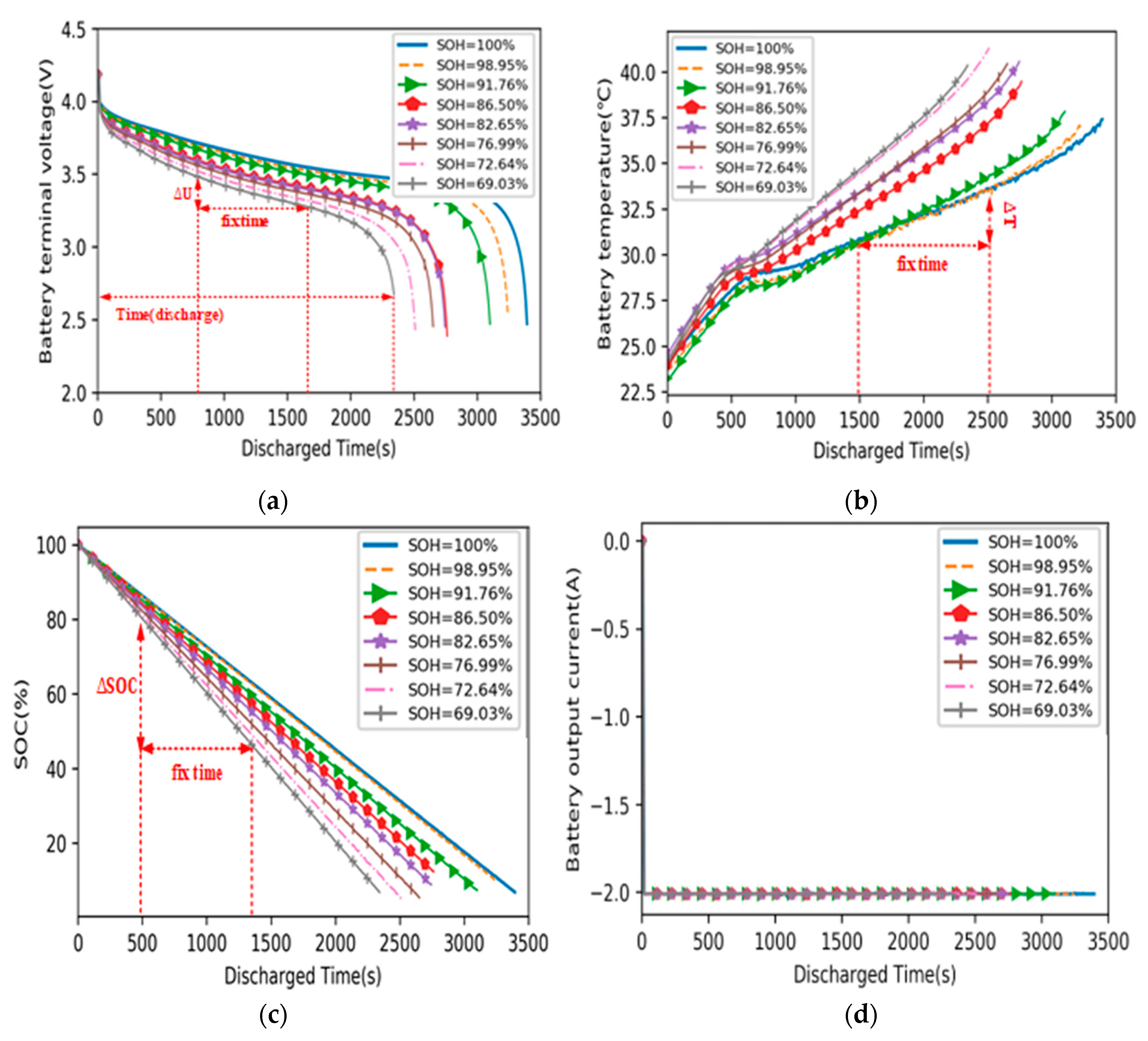
Feature selection is of great importance in SOH estimation of lithium-ion batteries, Figure 2 shows the change curve of characteristics with time under different health conditions.
The average voltage (U_ave) is defined as follows:
U _ a v e = U 0 U e T i m e ,
Among them, U 0 represents the starting voltage of the battery cycle once, U e represents the ending voltage of the battery cycle once, and Time represents the time of the battery cycle once.
Figure 2a shows the voltage change curve of lithium-ion battery under different health conditions. It can be seen from the figure that under different SOH levels, the average voltage (U_ave) of lithium-ion batteries is not equal. This means that the health status of lithium-ion battery affects the average voltage (U_ave), that is, the average voltage (U_ave) can reflect the health status of the battery to a certain extent. Therefore, the average voltage (U_ave) in the discharge process is used as the aging characteristics of the battery.
The voltage difference (∆U) represents the arbitrary voltage change in a short fixed time interval. It also can be seen from Figure 2a that the voltage difference (∆U) in a fixed time increases with the decrease of SOH. Since the internal resistance of the battery increases with the aging of the battery. Therefore, the voltage difference (∆U) can also be used as the aging characteristics of batteries.
The temperature difference (∆T) represents the arbitrary temperature change in a short fixed time interval. Figure 2b shows the temperature change curve of lithium-ion battery under different health conditions. It can be seen from the figure that the temperature increment in a fixed time will increase with the decrease of SOH. Since with the aging of the battery, the internal resistance of the battery increases continuously, and the heat generated in the chemical reaction process increases. Therefore, the temperature difference (∆T) can also be used as the aging characteristics of batteries.
It can be seen from Figure 2c that in a fixed period of time, the SOC goes down as the SOH keeps decreasing. Since the SOC drops, it will inevitably affect the discharge capacity of the battery, that is to say, SOC can reflect the health state of the battery to a certain extent. However, SOC is not generally used as a feature to predict SOH, it is often corrected according to the SOH values.
Figure 2d shows the current curve of lithium-ion battery under different health conditions. It can be seen from the figure that under different SOH levels, the current basically does not change. Therefore, the current difference can also be used as the aging characteristics of the battery.
Therefore, the voltage difference, temperature difference, and average voltage for the same time interval are used as the aging characteristics of batteries.

2.2. The XGBoost Model of SOH Estimation

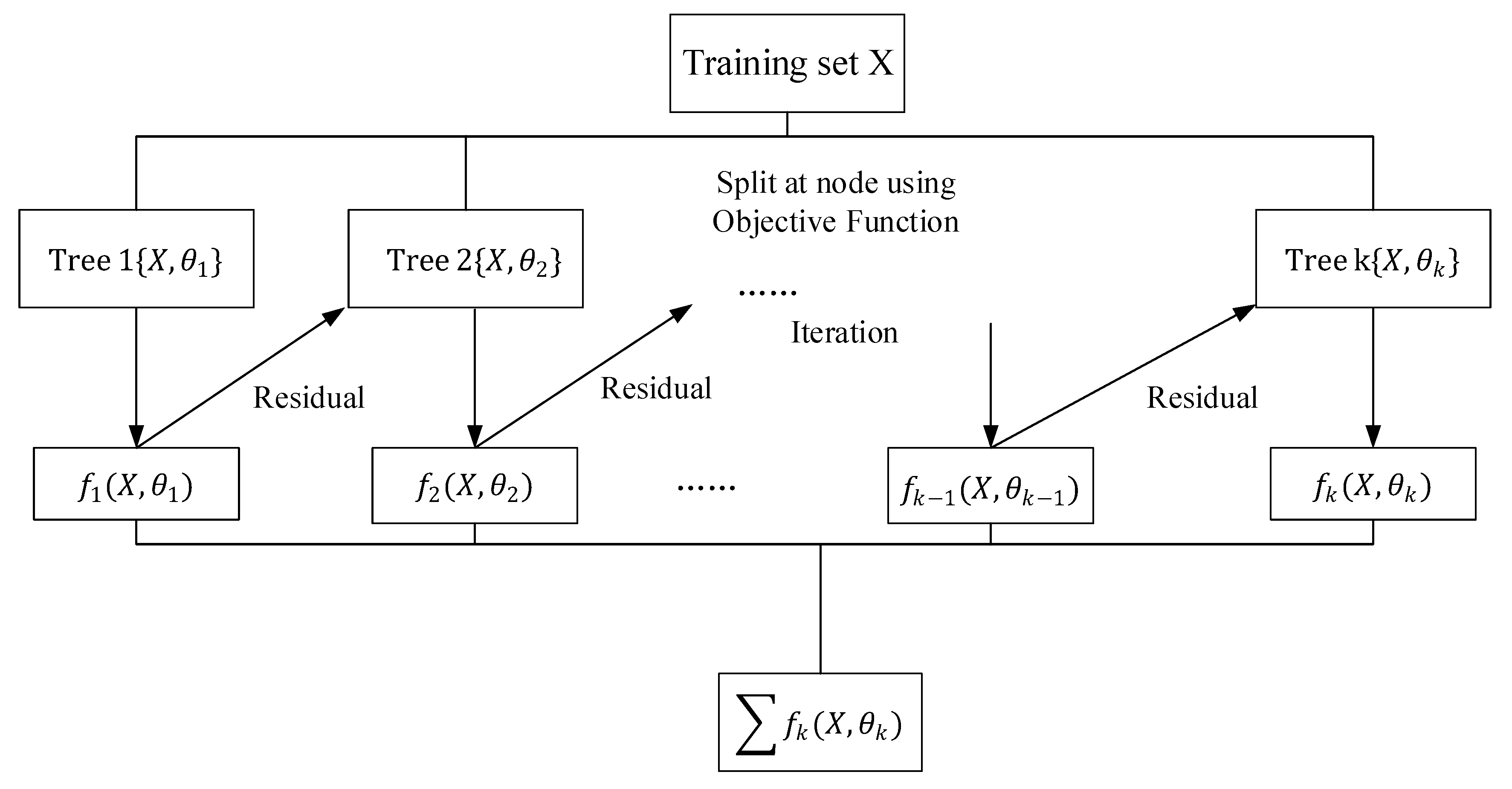
XGBoost adds split features to generate a tree. It is to learn a new function f (x) to fit the residual of the last prediction. When the k-th tree is trained, it is necessary to predict the score of a sample. According to the characteristics of the sample, it will fall on the corresponding leaf nodes in each tree. Each leaf node corresponds to a score. Finally, the corresponding score of each tree is added up as the predicted value of the sample, as shown in Figure 3.
XGBoost modeling: Give a generalized definition of objective function, find a suitable regression tree in each iteration to fit the residual of the last prediction, so that the objective function is further minimized, and the predicted value is closer and closer to the real value.
For example, data ( [ Δ U 1 , Δ T 1 , U a v e 1 ] , S O H 1 ), ( [ Δ U 2 , Δ T 2 , U a v e 2 ] , S O H 2 ),…, ( [ Δ U i , Δ T i , U a v e i ] , S O H i ), i = 1, 2,…, n. Among them, Δ U i , Δ T i , U a v e i and S O H i , respectively represent the voltage difference, temperature difference, average voltage, and health status corresponding to group I data.
We define the tree f t ( x i ) as follows:
f t ( x i ) = ω q ( x ) , q : Τ , ω T ,
where q represents the structure of each tree, it can map each sample to the corresponding leaf nodes, and T is the number of leaf nodes in the tree. Each ft corresponds to an independent tree structure q and leaf weight w.
In order to standardize the improved objective function, we define tree complexity Ω ( f t ) :
Ω ( f t ) = γ Τ + 1 / 2   λ j = 1 T w j 2 ,
where w j is the weight of the jth leaf node.
The objective function is defined as:
o b j ( t ) = i = 1 n l ( S O H i , S O H ^ i ) + k = 1 K Ω ( f k ) = i = 1 n l ( S O H i , S O H ^ i ( t 1 ) + f t ( Δ U i , Δ T i , U a v e i ) ) + Ω ( f t ) + c ,
Among them, i = 1 n l ( S O H i , S O H ^ i ) is the residual of the predicted value and the actual value of the model. f t ( Δ U i , Δ T i , U a v e i ) represents the model to be added to the decision of the t-round. k = 1 K Ω ( f k ) is a penalty term for the complexity of each model. f k is the model function of the tree and c is a constant.
The second-order Taylor’s formula is expanded and the objective function is as follows:
o b j ( t ) i = 1 n [ l ( S O H i , S O H ^ i ( t 1 ) ) + g i f t ( Δ U i , Δ T i , U a v e i ) + 1 / 2 h i f t 2 ( Δ U i , Δ T i , U a v e i ) ] + Ω ( f t ) + c , among   them ,   g i = S O H ^ i ( t 1 ) l ( S O H i , S O H ^ i ( t 1 ) ) , h i = S O H ^ i ( t 1 ) 2 l ( S O H i , S O H ^ i ( t 1 ) ) ,
The new objective function can be defined as:
O b j ( t ) = j = 1 T [ ( i I j g i ) w j + 1 / 2 ( i I j h i + λ ) w j 2 ] + γ Τ = j = 1 Τ [ G i ω j + 1 / 2 ( H i + λ ) ω j 2 ] + γ Τ ,
Define the candidate feature set of splitting nodes of each tree as I j , I j = { i | q ( Δ U i , Δ T i , U a v e i ) = j } .
The optimal weight ω j * of leaf node j and the optimal objective function solution o b j ( * ) :
ω j * = G i / ( H i + λ ) ,   o b j ( * ) = 1 2 j = 1 Τ G i 2 / ( H i + λ ) + γ Τ ,
Among them, G i = i I j g i ,     H i = i I j h i .
o b j ( * ) is a function of marking tree structure and measuring the quality of tree structure q. The smaller the value of o b j ( * ) , the better. In this way, the optimal segmentation point and the optimal decision tree structure can be obtained to minimize the objective function.
XGBoost is improved and optimized on the basis of GBDT [19]. Regular terms are added to the objective function of each iteration to control the complexity of the model and support column sampling, it can not only reduce over-fitting, but also reduce calculation. Compared with the iteration principle of GBDT heuristic, the optimization criterion of XGBoost is based on the minimization of the objective function, and uses second-order Taylor expansion to support custom cost function. XGBoost blocks and sorts each feature, which makes it possible to parallel computing when searching for the best segmentation point. At the same time, by setting a reasonable block size, it makes full use of the CPU cache to speed up reading, and the speed of data reading is faster. When the eigenvalues are missing, XGBoost can also automatically learn the direction of node splitting.

2.3. Markov Chain Correction

Markov chain, also known as discrete-time Markov chain, is a stochastic process in which state space transitions from one state to another. This process requires a “no memory” nature, that is, the probability distribution of the next state can only be determined by the current state, and is independent of the events before it in the time series. Assuming that the sequence state is X t 2 , X t 1 , X t , X t + 1 , then the conditional probability in state X t + 1 depends only on state X t , i.e.,
P ( X t + 1 | X t 2 , X t 1 , X t ) = P ( X t + 1 | X t ) ,
(1) Partition interval
The difference between the real data and the predicted data is called the relative estimation. The relative estimation of the SOH of the lithium-ion battery is calculated, X represents the relative estimation, and the relative estimations are normalized:
x ¯ = ( x x m i n ) / ( x m a x x m i n ) ,
According to the golden section method, the normalized values of relative estimation are divided into three states: E 1 , E 2 , and E 3 , and the three states are inversely normalized to the relative estimation sequences by the above formula. The relative estimation can be divided into three intervals ( S 1 , S 2 , S 3 ) .
(2) The computation of state transition matrix
The transition probability P i j is a one-step transition probability representing the transition probability of state i to state j, and the equation is expressed as follows:
P i j = c i j / C i ,
where c i j represents the access frequency from state i to state j between two adjacent cycles, and C i represents the number of states moving from state i between two adjacent cycles. The state transition matrix is:
P = [ P 11 P 12 P 13 P 21 P 22 P 23 P 31 P 32 P 33 ] ,
Therefore, the transition matrix of the n-th step is P ( n ) = [ P ] n .
(3) Estimation correction
To further improve the estimation accuracy, Markov Chain is used to correct the estimation results obtained by the XGBoost model when the relative error between the predicted value and the true value is large. The correction is performed by the following equation.
S O H b = S O H p ( Δ a + Δ b ) / 2 ,
where Δ a and Δ b are the upper and lower limits of the estimation interval corresponding to their states of the relative estimation, S O H b indicates the corrected value, and S O H p indicates the value estimated by the XGBoost model.

2.4. The Implementation of the MC-XGBoost Method

As shown in Algorithm 1, the implementation of the MC-XGBoost method mainly has three steps: Data setting, XGBoost estimation process, and Markov correction process. The three steps are described in the following:
Steps 1: Preprocess the data and set various parameters, such as eta, max_depth, min_child_weight, seed, colsample_bytree, gamma, etc.
Steps 2: Set up training data and test data, use XGBoost algorithm to train the prediction model for SOH estimation. If it is not the optimal parameter, the error between the predicted value and the real value is large, it is necessary to reset the parameters, repeat the above operation, and adjust the parameters until the optimal parameters are obtained.
Steps 3: Calculate the relative residuals by comparing the predicted values obtained by the XGBoost model with the real ones, partition the normalized relative estimations according to the golden section method, and compute the state transition matrix to determine the next state. Then, the corrected values are obtained by using Equation (13).
Algorithm 1 The implementation of the MC-XGBoost Algorithms
1:Input: Dataset X = [ Δ U i , Δ T i , U a v e i ], i { 1, 2, …, n}, the loss function: l ( S O H i , S O H ^ i ) , the total number of sub-tree: T
2:Output: Predicted health status of lithium-ion batteries: S O H b ;
3:Repeat
4:Initialize the t-th tree f t ( x i )
5:Compute g i = S O H ^ i ( t 1 ) l ( S O H i , S O H ^ i ( t 1 ) )
6:Compute h i = S O H ^ i ( t 1 ) 2 l ( S O H i , S O H ^ i ( t 1 ) )
7:Use the statistics to greedily grow a new tree f t ( x i ) : o b j ( * ) = 1 2 j = 1 Τ G i 2 / ( H i + λ ) + γ Τ , among them, G i = i I j g i ,   H i = i I j h i
8:Add the best tree f t ( x i ) into the current model
9:Until all T sub-trees are processed
10:A strong regression tree based on all weak regression subtrees
11:Compute the S O H p based on the strong regression tree
12:Repeat
13:Normalize the relative estimations: x ¯ = x x m i n x m a x x m i n ; determine the status: E 1 , E 2 , E 3 ; calculate the transition matrix: P; correct the prediction results by Markov Chain: S O H b = S O H p ( Δ a + Δ b ) / 2
14Output S O H p based on Markov Chain

3. Experimental Results

The data used in our experiments comes from the NASA Ames Research Center [20]. In the process of stable discharge experiment, four lithium-ion batteries (5, 6, 7, and 18) were obtained by charging, discharging, and impedance, and two kinds of experiments were carried out. One group takes the discharge data of #5, #7, and #18 as the training set of the model, and the #6 discharge data is used to estimate the accuracy of the model. The other group uses the discharge data of #5, #6, and #18 as the training set of the model, and the discharge data of #7 is used for the precision estimation of the mode.
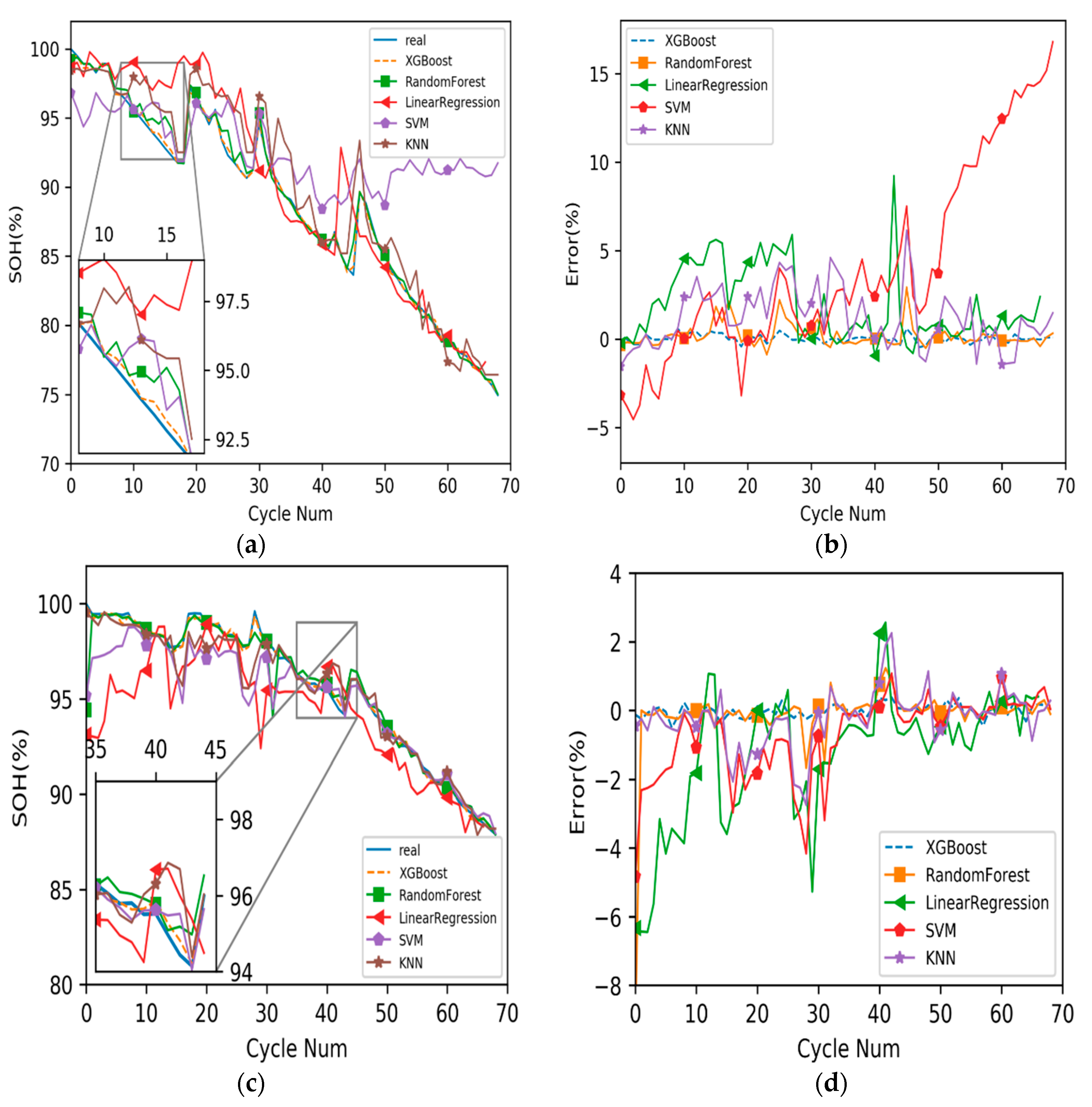
In order to verify the SOH estimation accuracy of lithium-ion batteries by the XGBoost method, we compare it with the Random Forest-based method, the Linear Regression-based method, the KNN-based method, and the SVM-based method on data set #6 and #7. Figure 4 shows the prediction results and prediction error of SOH on data set # 6 and #7.
The predicted results in Figure 4a show that on the #6 data set, the predicted results of linear regression, support vector machine, and KNN have obvious errors with the real values, while XGBoost and random forest have higher estimation accuracy in the latter estimation, but XGBoost is significantly closer to the real values than KNN in the earlier estimation. The prediction errors in Figure 4c shows that there are obvious errors between the predicted results of linear regression, support vector machine, random forest and KNN algorithm and the real values on the #7 data set, while the predicted results of XGBoost are close to the real values.
As shown in Figure 4b, the residual curves of XGBoost and random forest fluctuates up and down around 0 in the second half of the curve, but in the first half, the errors generated by the random forest fluctuates up and down far away from 0. Therefore, the estimation of random forest is not accurate in the early stage.
Table 1 shows that, the performances of the XGBoost method outperforms the other four methods on data set #6 and #7 in terms of mean absolute error (MAE), root mean square error (RMSE), and maximum error.
It can be seen from Table 1 that the values of XGBoost in three technical indexes are lower than those of the other four algorithms on data set #6 or #7.
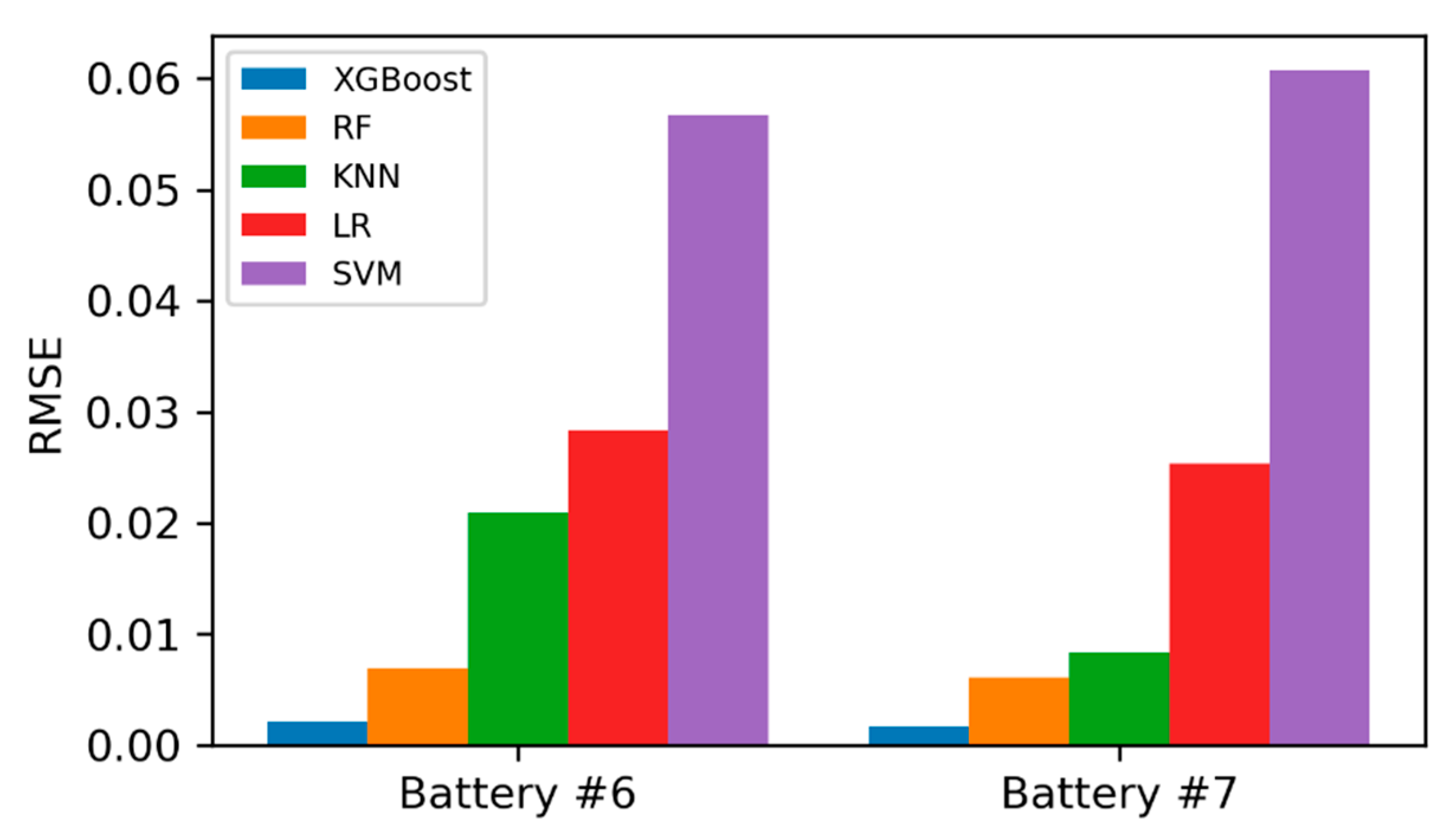
In conclusion, no matter on which data set #6 or #7 shown in Figure 5, the prediction results of XGBoost are almost close to the real values and have higher estimation accuracy.
The discharge process of lithium-ion battery is a time-varying process, and the change of its health state is a long-term process from the beginning of use to the end of life replacement. The state of health decreases with time, and the degree of health decreases. Markov chain has a significant prediction effect on the long-term system state, so we can correct the predicted errors by Markov chain to further improve the estimation accuracy by Markov chain.
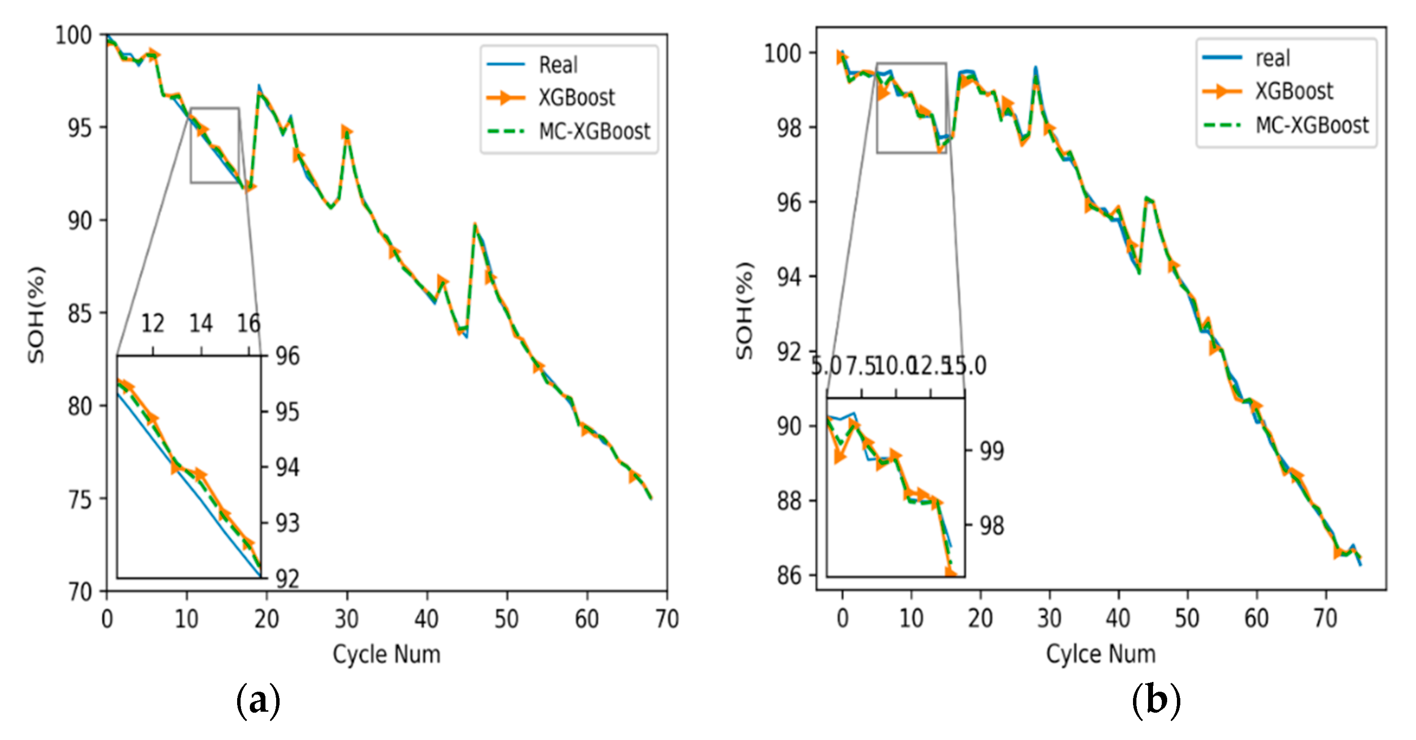
It can be seen from Figure 6 that XGBoost and MC-XGBoost both have a good prediction effect in the later stage, and the predicted values are close to the real ones. However, in the early stage, no matter on which data set #6 or #7, the predicted values under MC-XGBoost are closer to the real values than XGBoost.
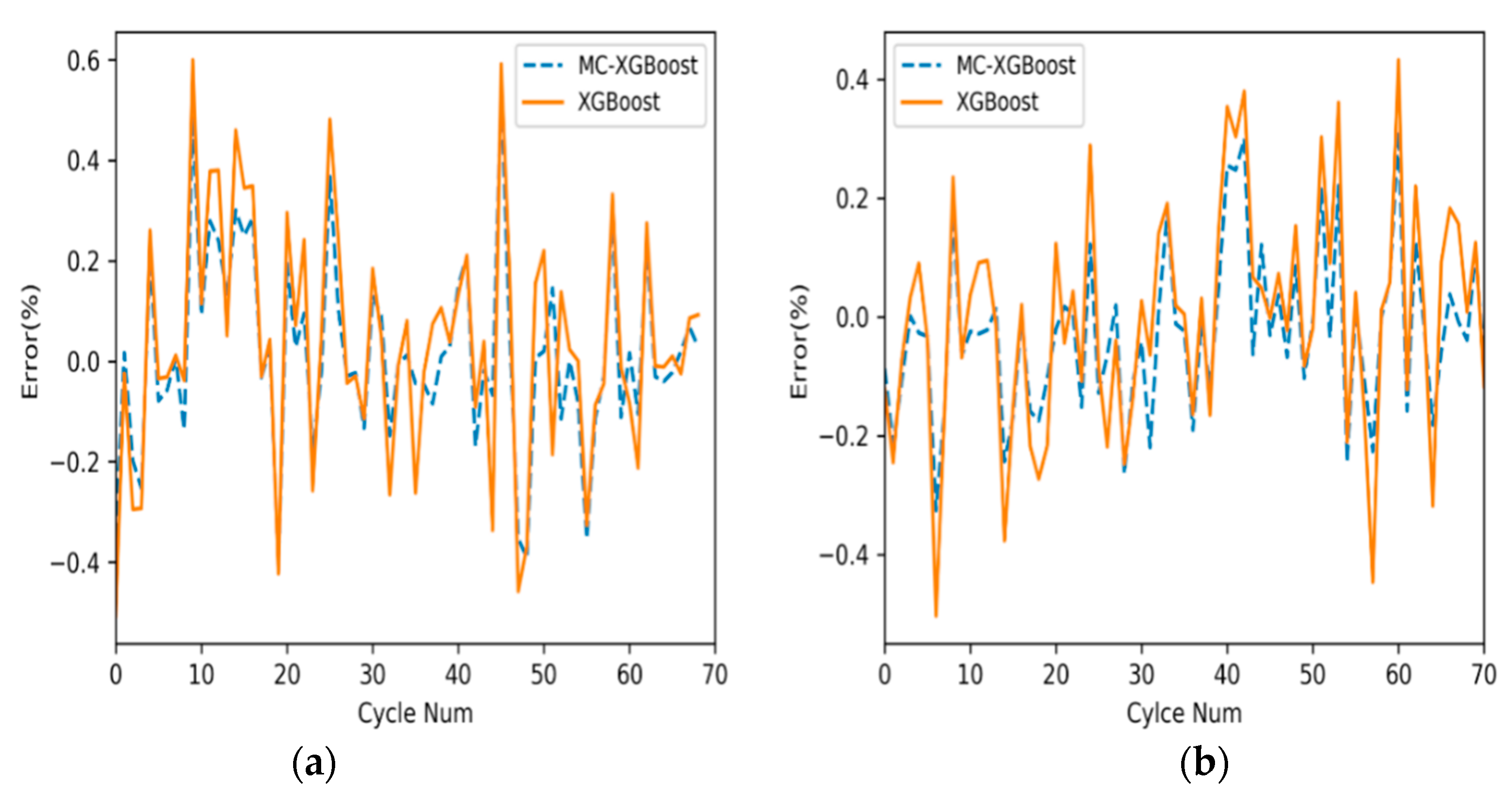
The prediction errors generated by MC-XGBoost and XGBoost methods are shown in Figure 7. No matter on which data set #6 or #7, the errors generated by the MC-XGBoost method fluctuate up and down near 0, and the fluctuation range is relatively small. Although most of the errors generated by XGBoost fluctuate up and down near 0, the fluctuation range is relatively large.
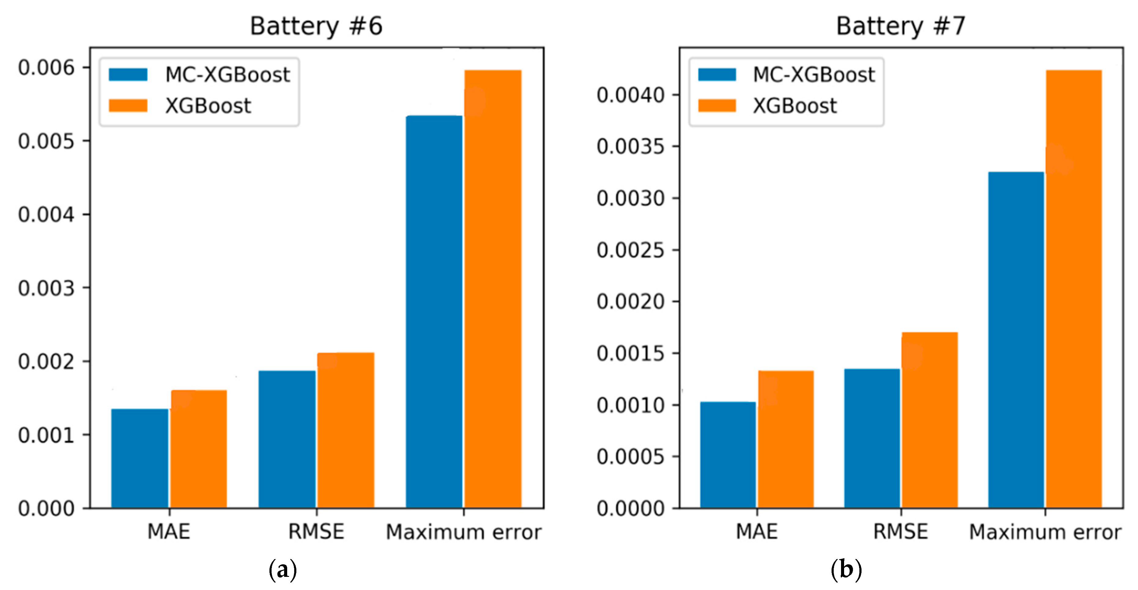
The MAE of MC-XGBoost and XGBoost is 0.001364 and 0.001615, respectively on data set #6, and 0.001035 and 0.001336, respectively on data set #7. The RMAE of MC-XGBoost and XGBoost is 0.001878 and 0.002132, respectively on data set #6, and 0.001355 and 0.001712, respectively on data set #7. The maximum error of MC-XGBoost and XGBoost is 0.005355 and 0.005972, respectively on data set #6, and 0.003263 and 0.004244, respectively on data set #7, as shown in Figure 8.
Compared with the XGBoost method, the MC-XGBoost method reduces the maximum error from 0.005972 to 0.005355 on data set #6 and 0.004244 to 0.003262 on data set #7 as shown in Figure 8. Therefore, compared with the other five algorithms, MC-XGBoost has a small error fluctuation range and can guarantee the stability of SOH prediction.
The MC-XGBoost method decreases by 15.5%, 22.5% in MAE, and by 11.9%, 20.8% in RMSE compared with the XGBoost-based method. That is to say, the performance ranks of the MC-XGBoost method and the other five methods is the MC-XGBoost method, the MC-XGBoost method, the XGBoost-based method, the RF-based method, the KNN-based method, the LR-based method, and the SVM-based method. Therefore, the Markov correction is effective in improving the accuracy of the predicted values.
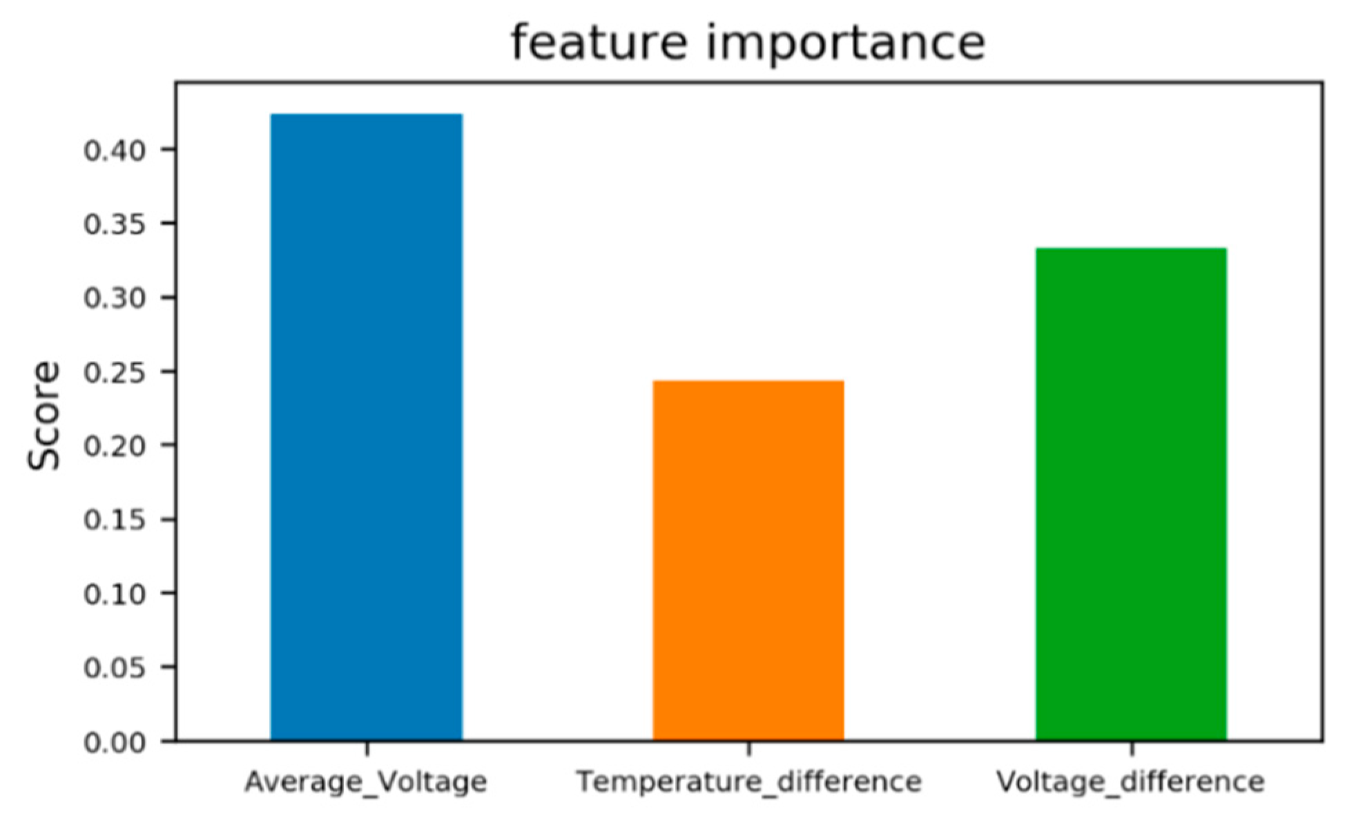
Figure 9 analyzes the contributions of the features to the SOH prediction. Among them, the average voltage has the greatest influence on the accuracy of the SOH prediction, followed by the voltage difference, and the temperature difference is the smallest. The feature importance ranking in SOH prediction is: Average voltage, voltage difference, temperature difference.

4. Conclusions

This paper presented a method for estimating the SOH using XGBoost algorithm with accuracy correction. Three battery features including the average voltage, voltage difference, and temperature difference are used to predict the SOH of lithium-ion batteries. SOH is first predicted by XGBoost algorithm, and then Markov chain is established to correct the predicted values. To verify the effectiveness of XGBoost, we compare XGBoost with five regression algorithms. The XGBoost algorithm has a high prediction accuracy, and strong generalization ability. The comparison between Markov correction and XGBoost shows that the Markov correction can significantly improve the prediction accuracy of XGBoost by 10%–20%. In addition, experiments on #6 and #7 battery data sets verify the generality of this method. In all, the experimental results show that the SOH prediction accuracy of the MC-XGBoost method is superior to the other five methods in three technical indicators, and the proposed method has higher SOH estimation accuracy.

Author Contributions

Conceptualization, S.S., C.F., H.X.; data curation, S.S., C.F.; formal analysis, S.S., C.F., H.X.; methodology, S.S. and C.F.; software, C.F.; supervision, S.S.; validation, C.F., H.X.; writing—review and editing, S.S., C.F. All authors have read and agreed to the published version of the manuscript.

Funding

This work is supported by the science and technology major project of Guangxi, under grant number AA18118009.

Conflicts of Interest

The authors declare no conflict of interest.

References

  1. Paul, N.; Wandt, J.; Seidlmayer, S.; Schebesta, S.; Mühlbauer, M.J.; Dolotko, O. Aging behavior of lithium iron phosphate based 18650-type cells studied by in situ neutron diffraction. J. Power Sources 2017, 345, 85–96. [Google Scholar] [CrossRef]
  2. Weng, C.; Feng, X.; Sun, J.; Peng, H. State-of-health monitoring of lithium-ion battery modules and packs via incremental capacity peak tracking. Appl. Energy 2016, 180, 360–368. [Google Scholar] [CrossRef] [Green Version]
  3. Weng, C.; Feng, X.; Sun, J.; Ouyang, M.; Peng, H. Battery SOH Management Research. In Proceedings of the 4th IFAC Workshop on Engine and Powertrain Control, Simulation and Modeling (ECOSM 2015), Ohio State University, Columbus, OH, USA, 23–26 August 2015; Volume 48. [Google Scholar]
  4. Moura, S.J.; Krstic, M.; Chaturvedi, N.A. Adaptive PDE observer for battery SOC/SOH estimation. In Proceedings of the ASME 5th Annual Dynamic Systems and Control Conference Joint with the JSME 11th Motion and Vibration Conference (DSCC2012-MOVIC2012), Fort Lauderdale, FL, USA, 2012; pp. 101–110. [Google Scholar]
  5. Ramadass, P.; Haran, B.; White, R.; Popov, B.N. Mathematical modeling of the capacity fade of Li-ion cells. J. Power Sources 2003, 123, 230–240. [Google Scholar] [CrossRef]
  6. Ng, K.S.; Moo, C.S.; Chen, Y.P.; Hsieh, Y.C. Enhanced coulomb counting method for estimating state-of-charge and state-of-health of lithium-ion batteries. Appl. Energy 2009, 86, 1506–1511. [Google Scholar] [CrossRef]
  7. Zhang, J.; Lee, J. A review on prognostics and health monitoring of Li-ion battery. J. Power Sources 2011, 196, 6007–6014. [Google Scholar] [CrossRef]
  8. He, Z.; Gao, M.; Wang, C.; Wang, L.Y.; Liu, Y. Adaptive state of charge estimation for Li-ion batteries based on an unscented Kalman filter with an enhanced battery model. Energies 2013, 6, 4134–4151. [Google Scholar] [CrossRef] [Green Version]
  9. Sánchez, L.; Couso, I.; González, M. A design methodology for semi-physical fuzzy models applied to the dynamic characterization of LiFePO4 batteries. Appl. Soft Comput. 2014, 14, 269–288. [Google Scholar] [CrossRef]
  10. Hoenig, S.; Singh, H.; Palanisamy, T.G.; Eagan, M. Method and Apparatus for Predicting the Available Energy of a Battery. U.S. Patent 6,618,681, 9 September 2003. [Google Scholar]
  11. Liu, D.; Pang, J.; Zhou, J.; Peng, Y.; Pecht, M. Prognostics for state of health estimation of lithium-ion batteries based on combination Gaussian process functional regression. Microelectron. Reliab. 2013, 53, 832–839. [Google Scholar] [CrossRef]
  12. Chen, Z.; Mi, C.C.; Fu, Y.; Xu, J.; Gong, X. Online battery state of health estimation based on Genetic Algorithm for electric and hybrid vehicle applications. J. Power Sources 2013, 240, 184–192. [Google Scholar] [CrossRef]
  13. Widodo, A.; Shim, M.-C.; Caesarendra, W.; Yang, B.-S. Intelligent prognostics for battery health monitoring based on sample entropy. Expert Syst. Appl. 2011, 38, 11763–11769. [Google Scholar] [CrossRef]
  14. Patil, M.; Tagade, P.; Hariharan, K.S.; Kolake, S.M.; Song, T.; Yeo, T.; Doo, S.-G. A novel multistage Support Vector Machine based approach for Li ion battery remaining useful life estimation. Appl. Energy 2015, 159, 285–297. [Google Scholar] [CrossRef]
  15. Nuhic, A.; Terzimehic, T.; Soczka-Guth, T.; Buchholz, M.; Dietmayer, K. Health diagnosis and remaining useful life prognostics of lithium-ion batteries using data-driven methods. J. Power Sources 2013, 239, 680–688. [Google Scholar] [CrossRef]
  16. Klass, V.; Behm, M.; Lindbergh, G. A support vector machine-based state-of-health estimation method for lithium-ion batteries under electric vehicle operation. J. Power Sources 2014, 270, 262–272. [Google Scholar] [CrossRef]
  17. Zhou, Y.; Huang, M. Lithium-ion batteries remaining useful life prediction based on a mixture of empirical mode decomposition and ARIMA model. Microelectron. Reliab. 2016, 65, 265–273. [Google Scholar] [CrossRef]
  18. Chen, T.; Guestrin, C. XGBoost: A scalable tree boosting system. In Proceedings of the 22nd ACM SIGKDD Conference on Knowledge Discovery and Data Mining (KDD), San Francisco, CA, USA, 13–17 August 2016. [Google Scholar]
  19. Yang, S.; Wu, J.; Du, Y.; He, Y.; Chen, X. Ensemble learning for short-term traffic prediction based on gradient boosting machine. J. Sens. 2017, 2017, 1–15. [Google Scholar] [CrossRef]
  20. Saha, B.; Goebel, K. NASA Ames Prognostics Data Repository: Battery Data Set [DS/OL]; NASA Ames Research Center: Santa Clara County, CA, USA, 2007. Available online: http://ti.arc.nasa.gov/project/pRognostic-data-repository (accessed on 10 September 2017).
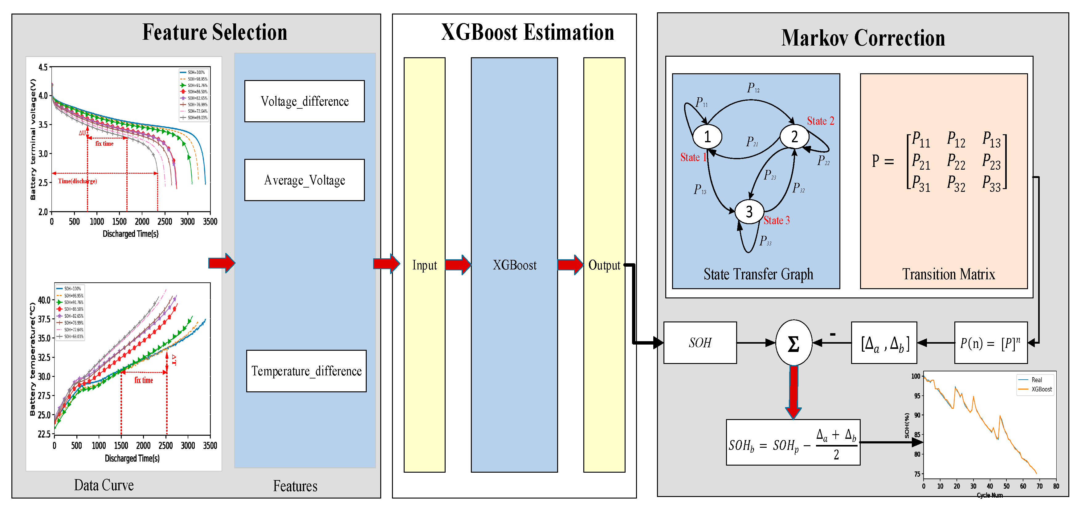
Figure 1. The flowchart of the MC-XGBoost method.
Energies 13 00812 g001
Figure 2. The characteristic curves under different SOH levels. (a) Voltage variation curve; (b) temperature change curve; (c) SOC change curve; (d) current change curve.
Energies 13 00812 g002
Figure 3. The flow chart of extreme gradient boosting.
Energies 13 00812 g003
Figure 4. The predicted results and prediction errors of SOH estimation on data set #6 and #7. (a) The predicted results of SOH estimation on data set #6; (b) the prediction errors of SOH estimation on data set #6; (c) the predicted results of SOH estimation on data set #7; (d) the prediction errors of SOH estimation on data set #7.
Energies 13 00812 g004
Figure 5. RMSE comparison by different methods.
Energies 13 00812 g005
Figure 6. The comparisons of the prediction results by the MC-XGBoost and XGBoost methods. (a) The prediction results on data set #6; (b) the prediction results on data set #7.
Energies 13 00812 g006
Figure 7. The comparisons of the prediction errors by the MC-XGBoost method and the XGBoost-based method. (a) The comparisons of the prediction errors on data set #6; (b) the comparisons of the prediction errors on data set #7.
Energies 13 00812 g007
Figure 8. The comparisons of three technical indicators by the MC-XGBoost method and the XGBoost-based method. (a) The comparisons of three technical indicators on data set #6; (b) the comparisons of three technical indicators on data set #7.
Energies 13 00812 g008
Figure 9. The importance of the battery features.
Energies 13 00812 g009
Table 1. The estimation results by the XGBoost method and the other four methods on data set #6 and #7.
MAEBattery #6 RMSEMaximum ErrorMAEBattery #7 RMSEMaximum Error
XGBoost0.0016150.0021320.0059720.0013360.0017120.004244
Random Forest (RF)0.0043790.0069470.0281830.0027160.0061080.059234
KNN0.0161930.0209370.0614880.0057320.0083870.027463
Linear Regression (LR)0.0202040.0283930.0922930.0165840.0253460.088665
SVM0.0455090.0567150.1185350.0533960.0608120.099835