Development of an Improved LMD Method for the Low-Frequency Elements Extraction from Turbine Noise Background

Abstract

Given the prejudicial environmental effects of fossil-fuel based energy production, renewable energy sources can contribute significantly to the sustainability of human society. As a clean, cost effective and inexhaustible renewable energy source, wind energy harvesting has found a wide application to replace conventional energy productions. However, concerns have been raised over the noise generated by turbine operating, which is helpful in fault diagnose but primarily identified for its adverse effects on the local ecosystems. Therefore, noise monitoring and separation is essential in wind turbine deployment. Recent developments in condition monitoring provide a solution for turbine noise and vibration analysis. However, the major component, aerodynamic noise is often distorted in modulation, which consequently affects the condition monitoring. This study is conducted to explore a novel approach to extract low-frequency elements from the aerodynamic noise background, and to improve the efficiency of online monitoring. A framework built on the spline envelope method and improved local mean decomposition has been developed for low-frequency noise extraction, and a case study with real near-field noises generated by a mountain-located wind turbine was employed to validate the proposed approach. Results indicate successful extractions with high resolution and efficiency. Findings of this research are also expected to further support the fault diagnosis and the improvement in condition monitoring of turbine systems.

1. Introduction

It has been clear that environmental pollution and scarcity of natural resources have been major factors affecting the sustainable development of human society. One significant part of these resource consumption and wastes discharge is the fossil-fuel based energy production and the associated greenhouse gas (GHG) emissions, which becomes a major concern regarding to the global climate change. Statistics conducted by the International Energy Agency (IEA) indicated that electricity production contributes up to 40% of global GHG emissions, which correspondingly results in a demand of 25,000 GW low-carbon energy by 2050 to satisfy sustainable living on the planet [1,2]. Recent studies revealed that given the negative environmental impacts result from fossil-based energy production, renewable energy sources such as wind turbines, concentrated solar power and solar photovoltaic could be desirable solutions for the sustainable energy production and supply. Regarding another study from the IEA, over 70% of the growth in global electricity production will be attributed to the renewable energy section, with the share of renewable energy estimated to increase by approximately 20–30% in 2023 [3]. As a clean, cost effective and low emission renewable energy source, wind power generated by turbines has found a wide application in green energy supply. According to the IEA studies mentioned above, wind energy harvesting could satisfy over 6% of the global energy demand by 2023.

Given the merits of lower emissions and cost in wind energy harvesting, however, concerns raised over the noises, especially the low-frequency noise emitted by turbines could not be overlooked. According to the statement of World Health Organization, health is defined as ‘a state of complete physical, mental, and social well-being and not merely the absence of disease or infirmity’. Therefore, noise annoyance and sleep disturbance as mentioned by van Kamp and van den Berge, are widely accepted as health issues [4]. Over the years, a considerable amount of studies have focused on the assessment of wind turbine noise, which results in an in-depth understanding of their impact on general health. Abbasi et al. claimed that noise exposure had a significant effect on general health, causing sleep disturbances and annoyance of people living close to wind farms [5]. This is further supported by a study conducted by Michaud et al., which indicated that annoyance would increase with the raising of noise levels around the wind turbines [6]. Findings obtained by Onakpoya et al. demonstrated that the odds of sleep disturbance increased significantly with greater exposure to wind turbine noise [7]. In addition, van Renterghem stated that wind turbine noises would become more annoying, when mixed with local road traffic noise [8].

On the other side, noise analysis takes a predominant role in the performance assessment and troubleshooting of wind turbines. The recent development of condition monitoring becomes an essential practice in wind farm monitoring, where noise and vibration signals are commonly employed as the data source for analysis and assessment. In the condition monitoring of wind turbines, aerodynamic noise is widely accepted as an important component due to its close interaction with abundant operating information of turbines [9]. However, a study conducted by Oerlemans indicated that the aerodynamic noise is often distorted by modulation due to the blade rotation, which might significantly affect the monitoring and analysis of turbine operating status [10]. Therefore, noise separation—especially the extraction of low-frequency noise—is the first and foremost step for a comprehensive understanding of turbine noise, as well as the monitoring of turbine health.

It is difficult to demodulate the aerodynamic noise of wind turbines, as it is generated by the interaction between air and impellers, which is often affected by fair pressure and vortex. In addition, the noise is normally mixed with neighborhood environmental noises such as sounds from birds, wind in trees and bushes, as well as local traffic noises, which make it difficult to take sufficiently precise measurement. Therefore, extraction of low-frequency elements from the noise background is difficult to be achieved with conventional approaches such as short-term Fourier transform (STFT), wavelet packet decomposition (WPD), Hilbert–Huang transform (HHT), empirical mode decomposition (EMD), local mean decomposition (LMD) and independent component analysis (ICA) [11]. Literature reviews indicate that STFT lacks adaptability with a fixed time-domain window used in the whole analysis process [12], WPD often suffers from the limitation of fixed basis functions [13], HHT usually decomposes signal into intrinsic mode functions, which affects the physical sense of noises [14], while the number of channels employed by ICA must be no less than the number of independent components [15]. As to the EMD, mode mixing is the major issue [16].

In light of the above, an improved local mean decomposition (LMD) method was developed in this study for the extraction of low-frequency noise, which can further support the fast identification of aerodynamic noise in condition monitoring. The rest of this paper is organized as follows: the composition of turbine noise with related characteristics are introduced in Section 2; followed by the LMD framework developed for noise extraction involved in Section 3. Section 4 presents the method employed for the measurement of turbine noise footprints, as well as the case study settings. Section 5 comes the results and analysis, with conclusion remarks and future works drawn to Section 6.

2. Wind Turbine Noise Composition and Characteristics

The sound of wind turbines is broadband and is unique in composition, due to its constantly moving characteristic and its being highly mixed with neighborhood environmental noises. It is different from the noises generated by conditioning fans and transportations, although some low-frequency and ‘movement’ characteristics are shared. Therefore, the understanding of wind turbine noises, which has been playing a predominant role in the impact assessment and fault finding of turbine systems, is significantly limited by the perception and measurement of sound, as well as the extraction of specified elements. It is well accepted that the sources of wind turbine noise can be classified into mechanical, aerodynamic and electromagnetic components. The mechanical element is generated by moving parts such as the gearbox, yaw gears and cooling fans, while the aerodynamic element is sourced from the interaction between blades and the airflow. As to the electromagnetic element, generators and other electrical equipment are the main contributors [17].

Regarding the decomposition of turbine noise, four elements are widely discussed: tonal, broadband, infrasound and low-frequency, as well as impulsive components, where the tonal noise might originate from non-aerodynamic structural resonances and meshing gears, or unstable flows over holes, slits and blunt trailing edges. Therefore, mechanical noise with mixed discrete frequencies is well accepted as tonal in character [18]. While broadband noise is identified as the result of interactions between trailing edges and boundary layer turbulence. Infrasound and low-frequency noise are produced by blades and air flow turbulence, while impulsive noise is mostly identified as the interactions of blades and disturbed air flow around the tower [17]. Current studies indicate that the aerodynamic noise of turbines is much more complex, as a mixture of all the four elements discussed above [19]. The generation of aerodynamic noise by turbine blades can be demonstrated in Figure 1.

As to the modelling and analysis of turbine noise, most studies indicated that the power of noise can be formulated as a function of wind velocity, where the strengths of elements are significantly affected by the rotor speed, modulated by the rotation rate of wind wheel [20,21]. The LMD proposed by Jonathan S. Smith is a novel iterative approach used in the demodulation of amplitude and frequency modulated signals, therefore it is a desirable solution for the processing of modulated signals [22]. Considering the highly mixed broadband characteristics of turbine noise, LMD was employed and improved in this research to eliminate the effects from the rotation rate of wind wheel and support the extraction of noise elements. Detailed methodology and operating strategies are discussed in the following sections.

3. Local Mean Decomposition

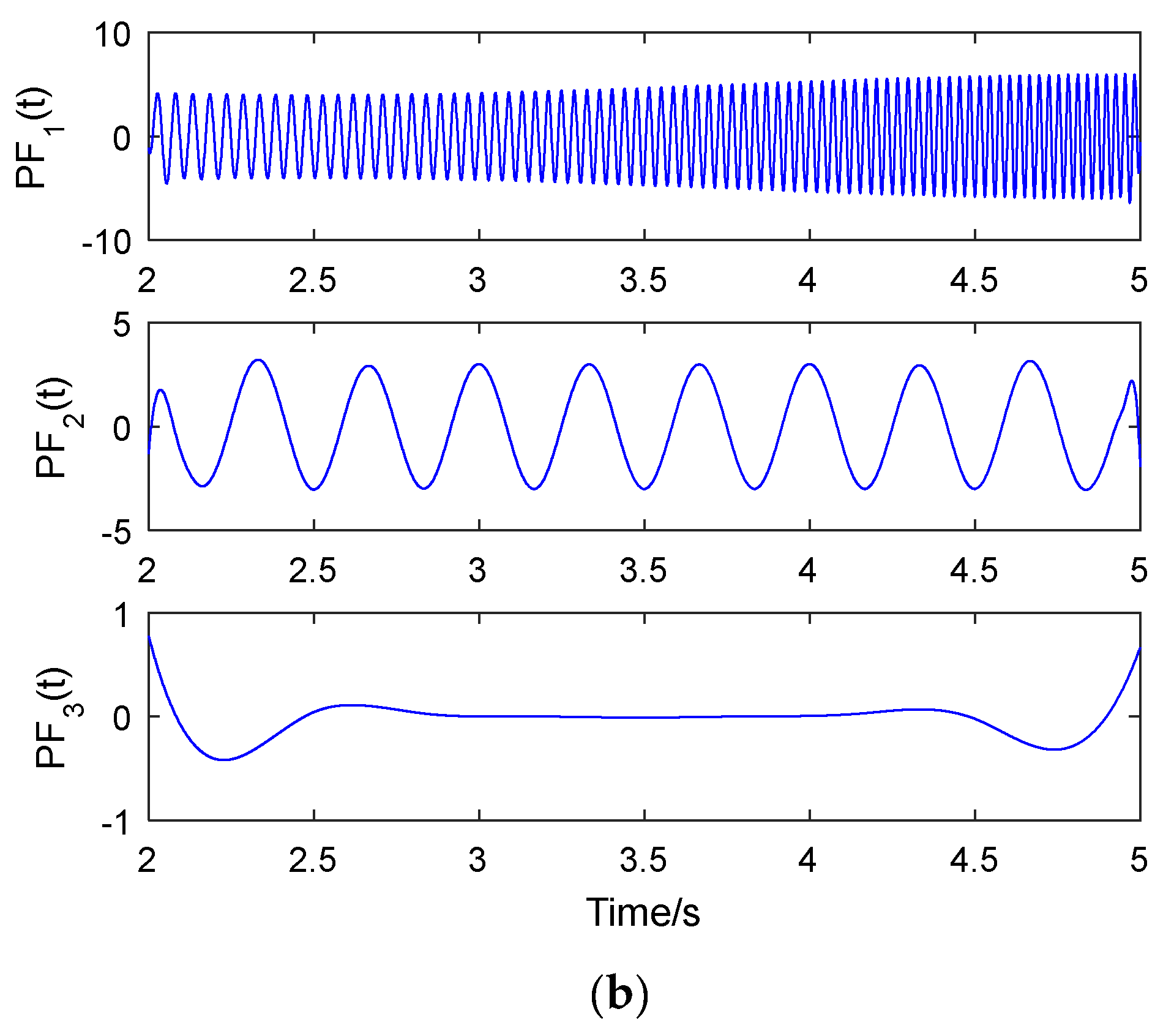
LMD is a self-adaptive decomposition method, which was initially developed to support the processing of multi-component modulated signals [23]. A literature review indicated that compared with EMD, LMD takes great advantages in processing instantaneous frequencies and interpreting signals with higher precisions [24]. In LMD operations, modulated signals are decomposed into a series of product functions (PF). As each PF is the product of an envelope signal and a frequency modulated signal, time-varying instantaneous phase and instantaneous frequency can then be obtained from the function [22]. Indeed, the LMD is achieved by moving the averaging method to gradually smoothed signals [25]. In this study, the improvement of LMD was primarily focused on computational efficiency, where spline envelopes are used to replace the moving averaging method in forming local means and local magnitudes. Therefore, the improved LMD still keeps the advantage of processing modulated signals. Figure 2 illustrated the framework for an LMD implementation. As for the LMD operations, a detailed scheme follows:

Extreme components of a serial signal are identified by the LMD algorithm; then the mean value of adjacent extremum points is calculated, followed by the obtain of the local mean values. After that the local magnitudes are smoothed by moving averaging. In this phase, the $i$^th mean value $m_i$ of two adjacent extremum points $n_i$ and $n_{i+1}$ is can be calculated with Equation (1):

$$m_i=\frac{n_i+n_{i+1}}{2}$$

(1)

while the local magnitude of the $i$^th half-wave oscillation can be expressed as:

$$a_i=\frac{\left|n_i-n_{i+1}\right|}{2}$$

(2)

With the identification of mean value $m_i$ and local magnitude $a_i$, the signal elements between points $n_i$ and $n_{i+1}$ are then allocated. After that, the local means and the local magnitudes are smoothed by moving averaging to form the smoothly varying continuous local mean function $m\left(t\right)$ and the envelope function $a\left(t\right)$.

In this step, the mean value is subtracted from the original data serial $x\left(t\right)$, and the resulting signal denoted by $h\left(t\right)$ is divided by the estimated envelope to form a new data serial $s\left(t\right)$. Here, if the obtained data serial $s\left(t\right)$ is not a purely frequency modulated signal, then reoperations would be conducted with $s\left(t\right)$ replaced by $x\left(t\right)$ in the loop. The looping cycles is determined by the subscript $q$. However, once a purely frequency modulated signal $s\left(t\right)$ was obtained, then the algorithm would be processed targeting product functions (PF). The number of product functions can be denoted by the subscript $p$. Equations (3) and (4) give the ways to generate $h\left(t\right)$ and $s\left(t\right)$, where both $p$ and $q$ equal to 1. Equation (5) shows the generating of $h\left(t\right)$ components in turn, where $p$ equals to 1 while $q$ varies from 1 to $n$. Equation (6) demonstrates the production of $s\left(t\right)$ components in turn, where $p$ equals to 1 while $q$ varies from 1 to $n$.

$$h_{11}\left(t\right)=x\left(t\right)-m_{11}\left(t\right)$$

(3)

$$s_{11}\left(t\right)=\frac{h_{11}\left(t\right)}{a_{11}\left(t\right)}$$

(4)

$$\{\begin{array}{c}{h}_{11}\left(t\right)=x\left(t\right)-m_{11}\left(t\right)\hfill \\ h_{12}\left(t\right)=s_{11}\left(t\right)-m_{12}\left(t\right)\hfill \\ ⋮\hfill \\ h_{1n}\left(t\right)=s_{1\left(n-1\right)}\left(t\right)-m_{1n}\left(t\right)\hfill \end{array}$$

(5)

$$\{\begin{array}{c}{s}_{11}\left(t\right)=\frac{h_{11}\left(t\right)}{a_{11}\left(t\right)}\\ s_{12}\left(t\right)=\frac{h_{12}\left(t\right)}{a_{12}\left(t\right)}\\ ⋮\hfill \\ s_{1n}\left(t\right)=\frac{h_{1n}\left(t\right)}{a_{1n}\left(t\right)}\end{array}$$

(6)

In this step, a corresponding envelope signal is obtained by multiplying the local magnitudes determined in the previous stage. After that, it would be multiplied by the frequency modulated signal to form a product function. The corresponding envelope is determined by Equation (7).

$$a_p\left(t\right)=a_{p1}\left(t\right)·a_{p2}\left(t\right)\cdots a_{pn}\left(t\right)={\displaystyle \prod }_{q=1}^n{a}_{pq}\left(t\right)$$

(7)

And the product function then can be expressed as:

$$P{F}_p\left(t\right)=a_p\left(t\right)·s_{pn}\left(t\right)$$

(8)

In the final stage, the product function is subtracted from the modulated signal as shown in Figure 2 once it has been formed; loops will be applied with the previous modulated signal replaced by the resulting signal until a constant is achieved or no more oscillation appears.

As discussed in the previous section, the moving averaging strategy is replaced by spline envelopes to improve the computational efficiency. In the classic LMD operating, moving averaging is a widely-used method to generate smooth-varying continuous local means and local magnitudes. However, it is generally computed costly as a looping algorithm, especially when nest loops are applied. In this study, with the employment of spline envelopes, only a single calculation is required for each envelop, which can significantly reduce the computational burden and improve the extraction efficiency. As demonstrated in Figure 3, in the improved LMD, local means are obtained from the summations of upper and lower envelope bounds, while local magnitudes are calculated based on the differential of upper and lower envelope bounds.

In addition, a classic LMD extracts local means by computing the mean values of each two successful extremes, and extending straight lines between successful extremes (as shown in Figure 4). After that, local means are smoothed by moving averaging to form the local mean function. To ensure the smoothness of local mean function, the values of two adjacent points must be different. Thus, normally four iterations are required to process the extreme points.

While, the improved LMD starts with the identification of the envelope upper and lower bounds, followed by averaging two envelopes to obtain the local mean function, thus, only one iteration is required (shown in Figure 5).

4. Wind Turbine Noise Measurement

To eliminate the interferences of other noises from the surrounding environment, the near-field noise of a wind turbine system was employed in this research to validate the proposed methodology. Due to the transient characteristics of natural wind, pure infrasound and low-frequency noises are difficult to obtain, which correspondingly affect the accurate description of turbine noise footprints. The selection of near-field noise for analysis is further supported by literature reviews. A study conducted Zhang et al. indicated that the levels of far-field turbine noise normally vary significantly with atmospheric conditions [26]. While another study claimed that when explored in high speed wind (normally > 10 m/s), turbine noise might be fully submerged by background noises [19]. Other impacts on turbine noise measurement might from the interference of neighborhood turbines, high residual noise of wind and unpredictable wind shear [27].

The near-field noise used in this research was collected from a wind turbine installed on a mountain located in middle China. The studied machine is a 2 MW wind turbine with variable pitch and direct-drive synchronous generator. The diameter of its wind wheel is 104.8 m and the height of its hub center is 80 m. As shown in Figure 6, the measure points are distributed along the hub central axis and perpendicular to the wind wheel plane. The first point was selected below the wind turbine wheel, other points are 5, 10, 15 and 20 m away from the wheel plane. The wind speed on the wind turbine nacelle was measured as 7.2 m/s to 12.4 m/s. The rotation rate of the wind wheel was approximate 14.5 rpm. Noise signals were acquired by LMS SCADAS data acquisition system equipped with Danish B&K microphones as shown in Figure 7, and the sampling frequency is 51,200 Hz. The specifications of SIEMENS LMS SCADAS data acquisition system are listed in

Table 1. Performance parameters of SIEMENS LMS SCADAS data acquisition system.

/ICP/Voltage Input	Maximum Sampling Rate	A/D Conversion	Vibration and Shock Resistance	AD Accuracy
40 channel	51.2 KHz	24 bits	Vibration resistance: >7 grms; shock resistance: >60 gpk	24 bits

. Due to the distance of measurement, the noise picked by microphone was considered from the blade near the tower.

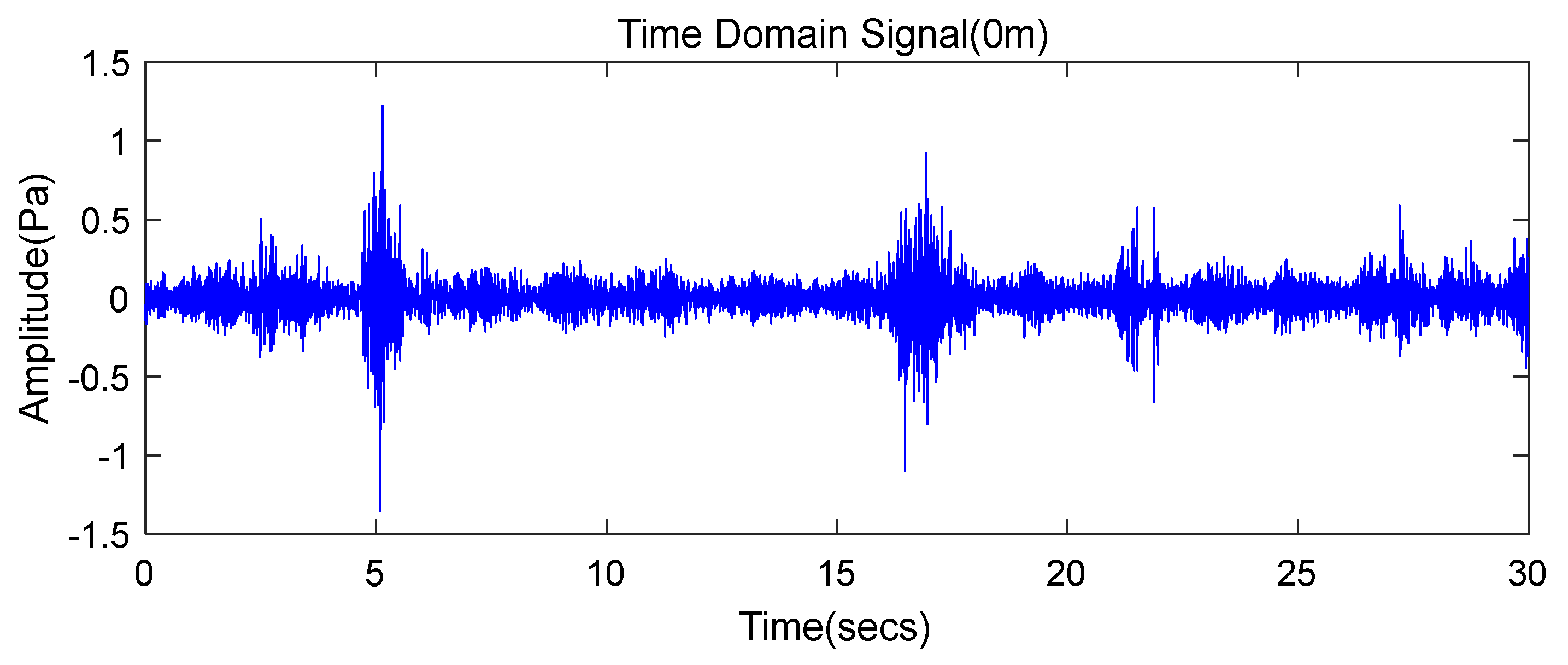
Existing studies indicated that a signal length of around 20 s seems to be an appropriate compromise to ensure stable statistics and get blade passing frequency [28]. However, considering the interference at the beginning and ending of the measurement, a 30 s signal recording was applied in this research. As the monitored wind turbine is a direct-driven system without gearbox, the mechanical noise which is mainly contributed by turbine gearboxes can then be eliminated. The time-domain noise signals recorded on the monitored wind turbine at measuring point 1 to 5 are presented in Figure 8, Figure 9, Figure 10, Figure 11 and Figure 12.

Previous studies found that noise propagated to the ground is emitted with the downward movement of blades excepting an insignificant source at the rotor hub [29]. That is validated by the frequency spectrum maps obtained in this research where low-frequency noises take the predominant role, as they are aerodynamic noise generated by the downward movement of blades. Figure 8 shows that the noise amplitude increased locally after 18–20 s recording, which is corresponded to the disturbance on the gust microphone. As shown in Figure 9, the change of wave-packets at monitoring point 2 illustrates that the forepart of diagram is dense while the posterior is sparse. Here the wave-packets are dense the wind wheel was rotating fast, and vice versa. Moreover, each wave-packet is corresponded to the noise of one blade passing through the tower. The rotating speed of wind wheel in the dense areas was 18 rpm, and that in the sparse areas was recorded as 14 rpm.

Monitoring point 3 involves two sharp high-amplitude signal lines as shown in Figure 10, which were identified as the impacts from the sound-picking microphone. Due to a significant increase of wind speed at monitoring point 4, the amplitude of noise signal shows a tendency of sharp increase. In addition, the increase of aerodynamic load on blades also contributed to the noise background. Simultaneously, with the rotation speed increased, the noise diagram demonstrates denser wave-packets compared with other moments. 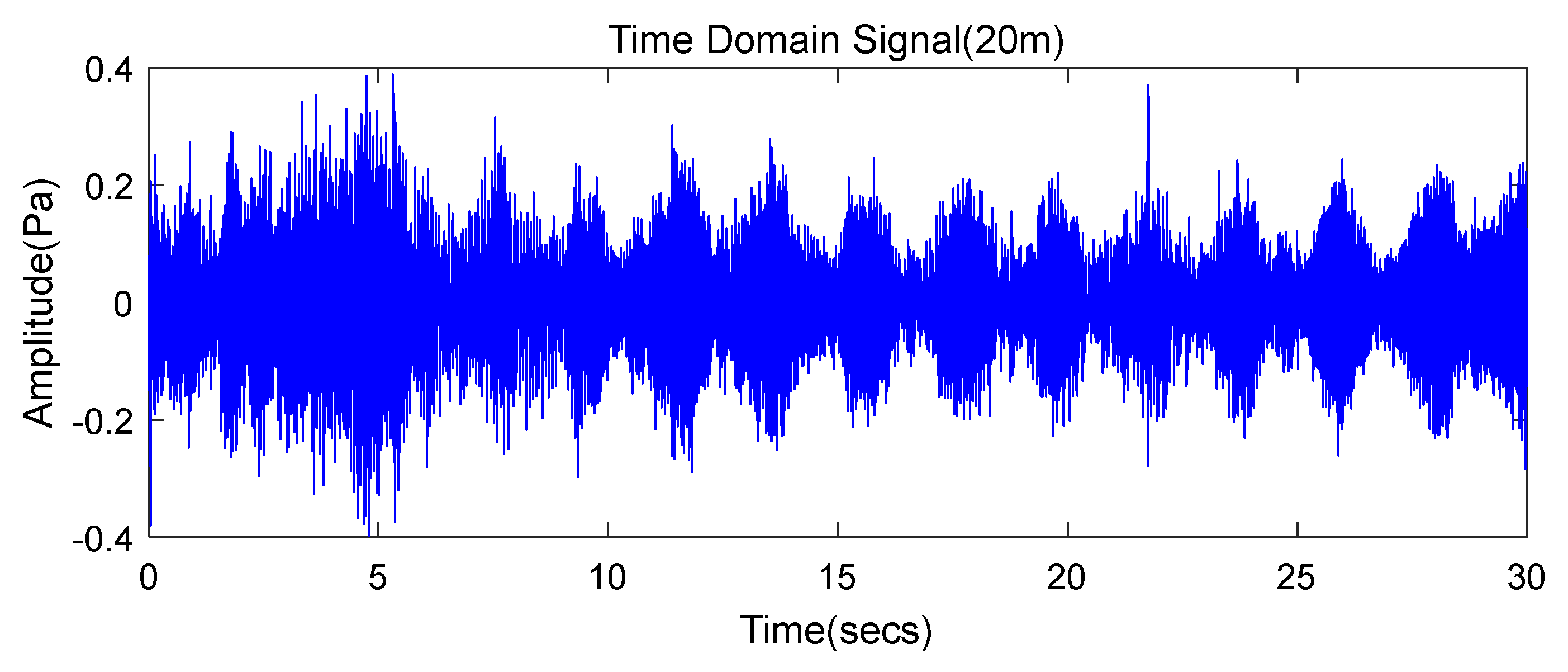Figure 12 shows the noise diagram obtained at monitoring point 5. The diagram demonstrates that after the initial fluctuations, the recorded signal at this moment becomes more stable, the difference between maximum amplitudes of wave-packets becomes insignificant, and the interval between wave-packets towards more uniform. This might attribute to the moving of wind speed from higher at the beginning to smooth later. Moreover, the high-amplitude peaks at around 13th second shown in Figure 11 and the high-amplitude peaks at around the 22nd second shown in Figure 12 result from an accidental turbulence picked up by the microphone.

5. Results and Discussion

5.1. Simulation Signal Analysis

A simulated signal $X\left(t\right)$ consisting of a frequency varying signal $x1\left(t\right)$, a frequency constant signal $x2\left(t\right)$ and a white Gaussian noise signal $x3\left(t\right)$ described as Equations (9)–(11), was employed in this research to validate the proposed methodology.

$$x1\left(t\right)=\left[5+\cos (0.4\mathsf{\pi }t)\right]\times \cos \left(14\mathsf{\pi }t+18t^2\right)$$

(9)

$$x2\left(t\right)=\cos (6\mathsf{\pi }t)$$

(10)

$$X\left(t\right)=x1\left(t\right)+3\times x2\left(t\right)+x3\left(t\right)$$

(11)

Figure 13 shows the time-domain diagrams of signal $X\left(t\right)$, $x1\left(t\right)$ and $x2\left(t\right)$.

For a comparative study to validate the proposed approach, the mixed simulation signal $X\left(t\right)$ was decomposed using classic LMD and the improved LMD respectively with three product functions obtained for each method. Waveforms described by the product functions are shown in Figure 14. Where PF₁ is corresponded to component signal $x1\left(t\right)$, and PF₂ is corresponded to triple of component signal $x2\left(t\right)$. While PF₃ is a fake component generated by the end-effect associated with the averaging moving processing. However, the white Gaussian noise could not be decomposed by either the classic or the improved LMD.

Figure 15 illustrates the errors between decomposed and original signals, here the deviations between PF₁ and $x1\left(t\right)$ is denoted by $d1\left(t\right)$, while the deviations between a third of PF₂ and $x2\left(t\right)$ is expressed as $d2\left(t\right)$. Figure 15b also indicates that the end-effect only affects the data close to the endpoints of PF₁ and PF_2, leaving the main parts of product functions are exactly consistent with the simulated signal components. In industrial operations, since a very limited amount of data is affected, the analysis of the main body signal remains under quality control when the recording is of acceptable length. Therefore, in some processing contexts which are insensitive to local signal loss, the data points near LMD endpoints are usually left out.

Table 2. Comparison of decomposition efficiency.

Method Used	Iteration Times	Time Consumption (s)
Classic LMD	12	0.33
Improved LMD	4	0.074

gives the iteration cycles and computation time spent with classic and improved LMDs respectively. Results indicate that the improved LMD is over four times faster than the classic LMD in decompositions. Therefore, the improved LMD proposed in this research is a desirable solution to extract low-frequency elements from the turbine noise background.

5.2. Monitoring Signal Analysis

Limited by the length of the article, two section noise signals of 5 s length which had been recorded at monitoring point 1 and point 2 were employed in this study to validate the developed methodology and demonstrate how it works. One signal recorded from the 4th second to the 6th second presented in Figure 8 and another signal recorded from the 5th second to the 10th second presented in Figure 9 were intercepted for analysis, with the time-domain and frequency-domain diagrams illustrated in Figure 16 and Figure 17. Here, the frequency band of the intercepted signal ranges from 0.1 Hz to hundreds of thousand Hz, with most large amplitude components distributed under the frequency of 600 Hz. The clear majority is between 10 Hz and 50 Hz, and the maximum amplitude point in Figure 16 is identified with the frequency of 34.2 Hz, while the maximum amplitude point in Figure 17 is obtained with the frequency of 27 Hz.

The improved LMD method was then used to decompose the intercepted signal at monitoring point 1 with seven product functions obtained from the extraction of the mixed noise emissions (last threes product functions’ diagrams shown in Figure 18), and the intercepted signal at monitoring point 2 with six product functions obtained from the extraction of the mixed noise emissions (last threes product functions’ diagrams shown in Figure 19).

Higher frequency components were extracted with priority, thus, the product functions obtained later are in fact the ones required in the analysis of infrasound and low-frequency noise of wind turbines. Product functions related to the maximum amplitude points in Figure 16 and Figure 17 were then processed with fast Fourier transform, with the frequency spectrum are presented in Figure 20 and Figure 21.

Results indicate that almost all those frequency components of PF₅ are under 100 Hz, with most of them between 10 and 40 Hz, including the maximum amplitude point found at frequency 34.2 Hz and 27 Hz. It then can be concluded that PF₅ covers most low-frequency noise and part of the infrasound under 20 Hz.

In light of the above, all those low-frequency components have been successfully decomposed from the monitoring noise signal using the improved LMD. Therefore, the improved LMD is of the ability to decompose wind turbine noise and to extract low-frequency components with high performance. Correspondingly, a successful extraction of low-frequency components from the wind turbine noise is of great importance in the understanding of their time-frequency characteristics. Moreover, understanding of the noise elements can further support the fault diagnosis of turbine systems, as well as to quantify the adverse impacts contributed by wind farms.

6. Concluding Remarks

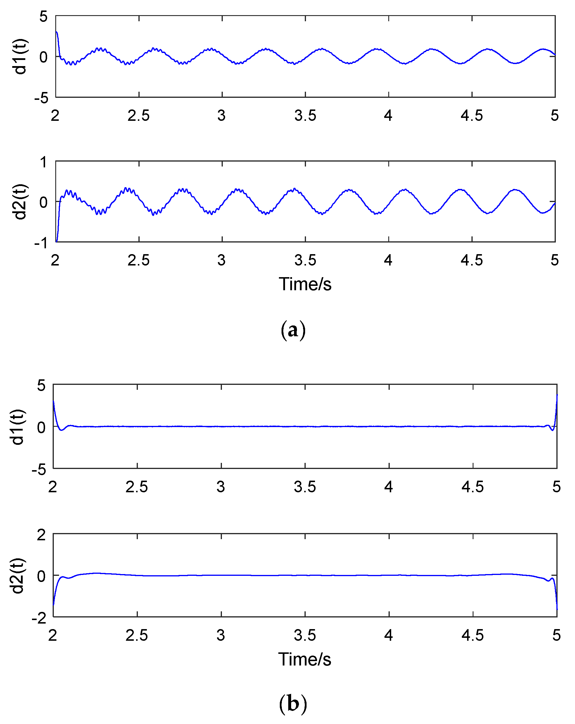
This research presents an improved LMD based approach for the extraction of low-frequency elements and infrasound from the noise of wind turbines. Simulation and experimental results indicate that the proposed method can separate noise signal effectively with high performance. As the extraction of noise elements is the milestone in the understanding of turbine aerodynamic noise, the findings of this research are expected to further support the fault diagnosis and improvement in condition monitoring of wind turbine systems. The improved LMD boosted the computational efficiency, which consequently contributed to the efficiency improvement in condition monitoring.

As the analyzed signal is just a part of the recorded noise, endpoint of the selected section might not be the global extremum of the original signal. Thus, if an endpoint is handled as an extremum point, or replaced by an estimated value in the extraction processing, errors might turn up. Moreover, since LMD is a loop algorithm, errors would be accumulated in the cycling process.

Over the years, a considerable amount of studies have been conducted to improve the decomposition efficiency of LMD. For example, a soft sifting stopping criterion has been proposed to automatically determine the optimal number of sifting iterations [30]; a signal extending approach based on self-adaptive waveform matching technique was applied to overcome the boundary distortion [31]; and a novel scheme used to automatically determine the fix subset size of the moving average algorithm by Liu et al. [32]. However, a desired solution is still difficult to achieve. Improvement usually means an increase of algorithm complexity, as well as processing time consumption. Meanwhile, the adaptability would also be limited with optimizations applied on endpoints processing. Although LMD is of the mentioned shortcomings, it is still an efficient method for decomposition of amplitude and frequency modulated signals, which has been validated in this study.

Future studies in this domain might focus on effective endpoints processing for LMD, fault diagnosis of turbine systems with specific noise elements, manufacturing improvements on turbine systems towards noise emission reduction, as well as quantitative assessment of the adverse impacts contributed by wind turbine systems.