Geographical Potential of Solar Thermochemical Jet Fuel Production

Abstract

The solar thermochemical fuel pathway offers the possibility to defossilize the transportation sector by producing renewable fuels that emit significantly less greenhouse gases than conventional fuels over the whole life cycle. Especially for the aviation sector, the availability of renewable liquid hydrocarbon fuels enables climate impact goals to be reached. In this paper, both the geographical potential and life-cycle fuel production costs are analyzed. The assessment of the geographical potential of solar thermochemical fuels excludes areas based on sustainability criteria such as competing land use, protected areas, slope, or shifting sands. On the remaining suitable areas, the production potential surpasses the current global jet fuel demand by a factor of more than fifty, enabling all but one country to cover its own demand. In many cases, a single country can even supply the world demand for jet fuel. A dedicated economic model expresses the life-cycle fuel production costs as a function of the location, taking into account local financial conditions by estimating the national costs of capital. It is found that the lowest production costs are to be expected in Israel, Chile, Spain, and the USA, through a combination of high solar irradiation and low-level capital costs. The thermochemical energy conversion efficiency also has a strong influence on the costs, scaling the size of the solar concentrator. Increasing the efficiency from 15% to 25%, the production costs are reduced by about 20%. In the baseline case, the global jet fuel demand could be covered at costs between 1.58 and 1.83 €/L with production locations in South America, the United States, and the Mediterranean region. The flat progression of the cost-supply curves indicates that production costs remain relatively constant even at very high production volumes.

1. Introduction

A goal set for this century is the transition of the transportation sector from a fossil energy base to a renewable one. This goal is mainly motivated by the necessity to limit climate change through a reduction of carbon dioxide emissions and by the limited long-term supply security of fossil fuels. This transition is very challenging to achieve as today by far the largest share of the energy used in this sector is provided by fossil fuels [1] and a switch to a radically different technology will necessarily involve large investments into infrastructure and propulsion technology [2]. Nevertheless, electro-mobility is projected to drastically increase its share in the ground-based transportation sector [1], which would enable one to mainly use electricity for the propulsion of light-duty vehicles. In heavy-duty and airborne transportation, liquid hydrocarbon fuels are an ideal energy carrier due to their high energy density and favorable handling properties, as well as the existing global supply infrastructure. Especially for aviation, a transition to hydrogen or batteries is not as easy to implement as for cars because of the much stricter requirements for low weight and the volume of the energy carrier. It is therefore desirable to produce a liquid hydrocarbon fuel from renewable primary energy that can be used with the current infrastructure and propulsion technology. Among the different options, the use of solar energy is promising due to its widespread availability and already existing economic conversion technologies into heat and electricity. In recent years, electrochemical and thermochemical pathways have shown interesting results. Here, the focus is on the latter due to its high energy conversion potential [3,4] and significant experimental progress [3,5,6,7].

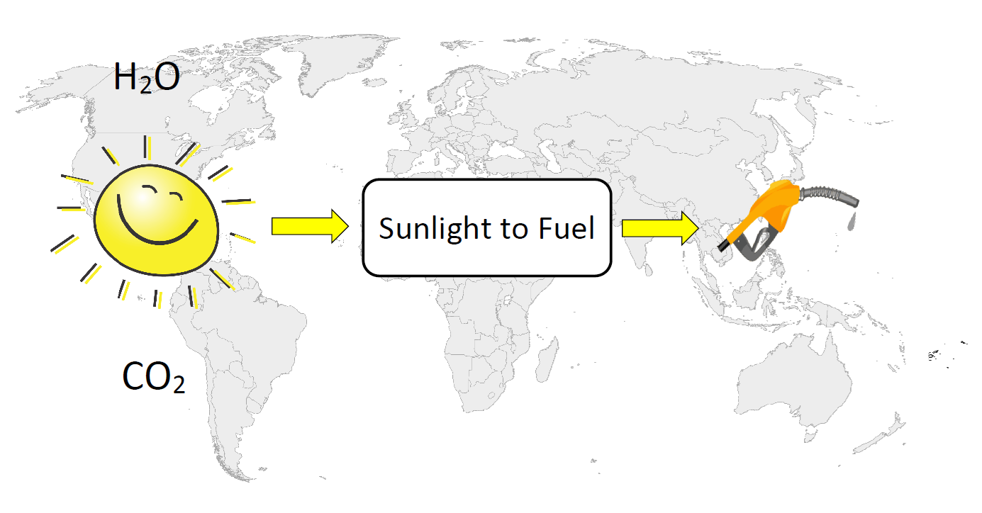
As solar energy is in principle able to cover the global energy demand, its conversion into liquid fuels could also easily cover the fuel demand of global aviation. As the production of solar thermochemical fuels requires only sunlight, water, and carbon dioxide, it could give a range of countries the possibility to produce their own environmentally-friendly fuels without having to rely on imports from oil-producing countries. However, as sunlight is unevenly distributed over the surface of the earth, there are regions that are more suitable for solar fuel production than others. It is therefore interesting to analyze the dependency of the fuel production costs on geographical location and to quantify the production potential in different regions of the earth.

In the literature, the geographical production potential of solar electricity with concentrated solar power (CSP) has been analyzed e.g., in [8,9,10,11,12,13,14] and that of PV electricity in [15]. The power-to-liquid (PtL) pathway uses water electrolysis to produce hydrogen and converts it with CO₂ to liquid fuels using reverse water gas shift and the Fischer–Tropsch process and is therefore technically related to the solar thermochemical pathway. The potential and cost of PtL fuels have been determined in [16,17,18,19] and it is found that the pathway is in principle scalable to meet the largest demands at costs of about 3.2 €/L today or 1.4 €/L assuming low-cost renewable electricity in 2050 [19]. To the best of the authors’ knowledge, the geographical potential in combination with the cost of solar thermochemical fuels have not been published so far, as only cost estimates exist for specific single locations. Thus, the focus is on the geographical variability of solar thermochemical fuel production characteristics. The theoretical amount of fuels that can be produced along with the estimated production costs for the most interesting regions of the earth is presented. To this end, a geographic information system (GIS)-based approach is used in combination with technical and economic models of the fuel production process. Studies have been performed on the geographical potential of solar technologies for electricity production [8,20,21], and on the potential of biogenic sustainable energy [22,23,24,25], but none on the particular case of solar thermochemical fuels. After the exclusion of unsuitable areas due to sustainability criteria, the linkage between production potential and production cost is shown on a regional and national level with cost-supply curves. With the information shown in this work, the regional and global potential for solar fuel production is quantified and the life-cycle costs for single regions and countries can be estimated, establishing a useful tool for decision-makers in the area of alternative fuels.

The Solar Thermochemical Pathway

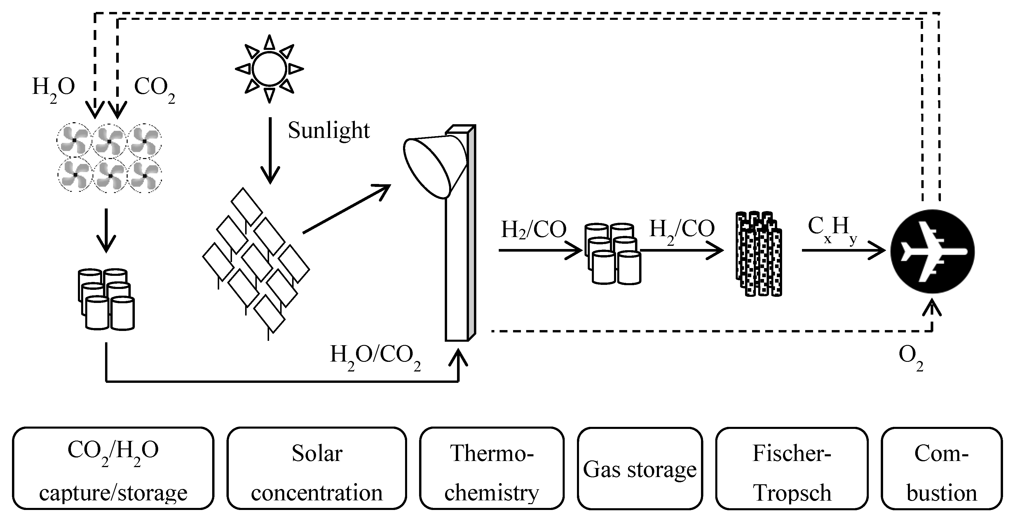
In the solar thermochemical pathway, solar energy is concentrated to provide heat to a redox cycle of a metal oxide operating between temperatures of about 1000 K and 1800 K. Cerium oxide is chosen as the reactive material, which is placed in a solar cavity reactor. Through the input of solar heat, the reactor is cyclically heated to the upper process temperature, where the material releases a part of its stored oxygen under a reduced oxygen partial pressure in the reactor. This is achieved through the removal of oxygen with a vacuum pump. In the second step of the cycle, the temperature of the reactor is reduced, and water and carbon dioxide are introduced, which are subsequently split into oxygen and synthesis gas (hydrogen and carbon monoxide). Cerium oxide returns to its initial state by absorbing the evolving oxygen, and the synthesis gas can then be converted into liquid fuels by the Fischer–Tropsch process. A schematic of the solar thermochemical fuel production process is shown in Figure 1.

The redox reactions are shown in Equations (1)–(3):

$$\frac{1}{{\delta }_{\mathrm{red}}-{\delta }_{\mathrm{ox}}}{\mathrm{CeO}}_{2-{\delta }_{\mathrm{ox}}}\to \frac{1}{{\delta }_{\mathrm{red}}-{\delta }_{\mathrm{ox}}}{\mathrm{CeO}}_{2-{\delta }_{\mathrm{red}}}+\frac{1}{2}{\mathrm{O}}_2$$

(1)

$$\frac{1}{{\delta }_{\mathrm{red}}-{\delta }_{\mathrm{ox}}}{\mathrm{CeO}}_{2-{\delta }_{\mathrm{red}}}+{\mathrm{H}}_2\mathrm{O}\to \frac{1}{{\delta }_{\mathrm{red}}-{\delta }_{\mathrm{ox}}}{\mathrm{CeO}}_{2-{\delta }_{\mathrm{ox}}}+{\mathrm{H}}_2$$

(2)

$$\frac{1}{{\delta }_{\mathrm{red}}-{\delta }_{\mathrm{ox}}}{\mathrm{CeO}}_{2-{\delta }_{\mathrm{red}}}+{\mathrm{CO}}_2\to \frac{1}{{\delta }_{\mathrm{red}}-{\delta }_{\mathrm{ox}}}{\mathrm{CeO}}_{2-{\delta }_{\mathrm{ox}}}+\mathrm{CO}$$

$$\begin{gathered} {\mathrm{H}}_2\mathrm{O}\to \frac{1}{2}{\mathrm{O}}_2+{\mathrm{H}}_2 \\ {\mathrm{CO}}_2\to \frac{1}{2}{\mathrm{O}}_2+\mathrm{CO} \end{gathered}$$

(3)

Water and carbon dioxide can in principle be provided from any source, whereas direct air capture is an attractive option for future implementations due to its environmental performance and the avoidance of long-range gas transport. Through chemical adsorption to a sorbent, both water and carbon dioxide are captured, whereas even in dry regions, the amount of water captured surpasses the amount of captured carbon dioxide [26]. The technology is currently in a demonstration phase with early commercial applications e.g., by Climeworks [27].

Solar thermochemical fuel production has been the subject of ongoing research and has experienced a significant increase in reactor efficiency from a value of 0.8% [5] in 2008 to 1.7% [6] in 2012, and most recently to above 5% [7] (at a potential exceeding 50% [28]). These results were achieved through an improved material and reactor design, enabling higher heat and mass transfer rates in the reactor. Especially the introduction of different length scales for the porosity of the reactive material has reduced the time scales for heating up the material, which reduces the required power input while maintaining a high surface area needed for quick reoxidation [3,6,7]. Further development of the technology is likely to comprise material morphology and the introduction of an effective heat exchanger to reduce the energy input to the cycle. Heat recuperation from the solid phase has been shown to be vital for the achievement of higher efficiencies due to the comparable small oxygen nonstoichiometry of non-volatile material cycles [4,29,30,31,32]. Several promising reactor designs exist that could further enhance the conversion efficiency by the incorporation of solid-solid heat exchange [31,33,34] and by using particles for higher flexibility of the design [35,36]. The material properties are also sought to be improved through doping with specific elements [28,37,38,39] or through completely new material combinations [40,41,42]. To achieve an economic production process, it is assumed that efficiency of roughly 20% has to be reached for the thermochemical conversion [43,44], whereas the exact value is subject to detailed economic modeling and also depends on economic and political framework conditions. While experimental values are still significantly below this threshold, theoretical analyses have shown that values even beyond 20% are possible [45].

2. Methodology

In this section, the methodology chosen for the determination of suitable areas and production costs of solar thermochemical fuels is described. In general, the analysis was limited to regions with a high level of direct normal irradiation (DNI), i.e., the USA, the Andes region in South America (including Chile, Bolivia, Argentina, and Peru), the Mediterranean region (MED; including Southern Europe, the Middle East, and North Africa), Southern Africa (including South Africa, Botswana, Angola, and Namibia), and Australia. First, a list of exclusion criteria was defined for the determination of the available areas. Then the remaining net areas were combined with the available DNI and a conversion factor to determine the production potential. In a second step, an economic model was applied to express the production costs of solar thermochemical fuels as a function of the location. In the following, these steps are discussed in more detail.

2.1. Determination of Suitable Areas for Solar Thermochemical Fuel Production

The software QGIS [46] was used as a GIS-based tool for the net area calculations. Similar to the calculations performed in the MED CSP study [8] for the determination of suitable areas for CSP plants in the Mediterranean, the following areas were excluded: areas with existing ground structures, water bodies, shifting sands, slopes ≥5%, protected areas, as well as areas covered by forest, closed shrubland, woody savannas, wetland, cropland, urban settlements, or snow/ice. Consequently, allowed land types are open shrubland, savannas, and barren or sparsely vegetated land that do not fall under the restrictions listed above. Regarding land cover, data from the University of Arizona were used with a resolution of 15 arc seconds that assigns each pixel a type of land coverage based on the highest confidence for the years 2001–2010 [47]. Vector data on protected areas are taken from the World Database on Protected Areas [48], a joint project of the United Nations Environment Program and the International Union for the Conservation of Nature. Protected areas comprise national protected areas recognized by the government, areas designated under conventions, privately protected areas, and community-conserved territories. The data on shifting sand dunes and quicksand is taken from the Food and Agriculture Organization of the United Nations (FAO) [49]. The vector graphics for country borders are retrieved from the Database of Global Administrative Areas (GADM) [50] and the coastlines are from the Global Self-consistent, Hierarchical, High-resolution Geography Database [51]. The slope data was derived from a digital elevation model of the National Oceanic and Atmospheric Administration (NOAA) [52].

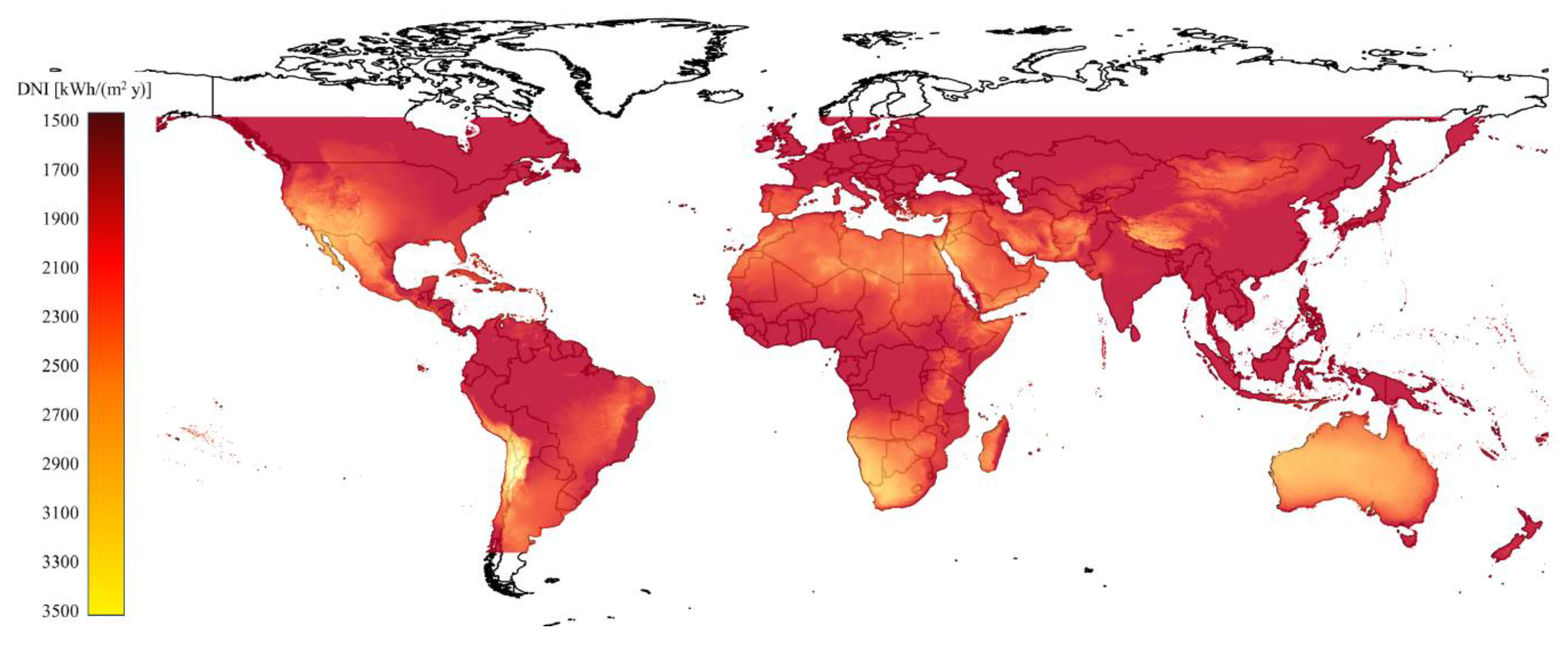
A map with the net available areas is created by subtracting all excluded areas described above. On the remaining land, the direct normal irradiation (DNI) is mapped with data from the Global Solar Atlas [53] with a resolution of 1 km². The data cover latitudes between 60° N and 45° S, whereas the incline of the satellite images prevents an accurate assessment of cloud covers outside of this area. Local DNI values are derived from a combination of a clear sky model that calculates the local solar energy flux based on the position of the sun, altitude, concentration of aerosols, water vapor content, and ozone, and satellite images that detect the cloud cover. The primary grid resolution is 3–7 km, which is downscaled to a resolution of 1 km. The satellite data represents the average DNI over a range of years, being 1999–2015 for the USA and South America, 1994–2015 for Europe and Africa, 1999–2015 for the eastern part of the MED region, and 2007–2015 for Australia.

2.2. Determination of Life-Cycle Production Costs

To determine the production costs of one liter of solar thermochemical jet fuel, an economic model was developed based on the levelized cost of energy (LCOE) [54]. The base year of the analysis is 2017.

Due to the long lifetime of the plant of 25 years, the time value of money has to be taken into account. This is achieved through the annualization of the investment and operational costs, which requires the definition of an interest rate. This interest rate is equivalent to the weighted average cost of capital (WACC) and is comprised of an equity rate and a debt rate. Consequently, the calculation of an annual value of the total costs of the plant is the sum of the annualized investment costs and the yearly operation and maintenance costs. The total annual costs are then divided by the annual production volume of fuel. Specifically, the equations used are the following:

$$\mathrm{LCOE}=\frac{I+P{V}_{\mathrm{O}\&\mathrm{M}}}{Q\times A}$$

(4)

I denotes the investment costs assumed to be paid at the beginning of the plant lifetime, PV_O&M is the present value of the operational costs of the plant, which accumulate over the lifetime, Q is the annual amount of fuel produced, and A = (1 − (1 + i)⁻ⁿ) i⁻¹ is the annuity factor. i denotes the interest rate and n the lifetime of the plant:

$$A=\frac{1-{\left(1+i\right)}^{-n}}{i}$$

(5)

The investment costs are assumed to be financed 60% through debt and 40% through equity, which is equivalent to a WACC of 0.6 d + 0.4e, with the interest rate for debt d and for equity e. The cost of debt and equity can vary substantially between countries due to differences regarding political, budgetary, and macroeconomic stability, as well as financial market efficiency [55]. However, it is not possible to determine the exact cost of debt and equity for a specific investment project, as this is determined by financial market actors. Rather, a meaningful comparison of country-specific cost of debt and equity needs to rely on suitable proxy indicators. Consequently, the weighted average costs of capital determined here should be understood as estimates. In the following, it is described which indicators, data sources, and methods are used.

The equity interest rate is assumed to be the sum of the government bond yields and an equity risk premium (ERP). Essentially, the ERP is an indication for “the compensation investors require to make them indifferent at the margin between holding the risky market portfolio and a risk-free bond” [56]. More specifically, one can assume that government bonds represent the benchmark for risk-free bonds. Thus, to estimate equity interest rates, one can sum up country-specific government bond yields with country-specific equity risk premiums. Government bond yield data are retrieved from different financial analyst organizations [57,58]. For the latter, data compiled by Damodaran [59] are used, whereas ERP values are calculated from mature market premiums, which are adapted by country risk premiums. Even though ERP values are hard to determine [60], the authors think that the dataset used here is adequate for the performance of a general comparison of the cost of capital across different countries. However, it is necessary to emphasize that diverse models and sources for ERP exist and that ERP estimates can vary substantially between sources [56,60]. For an in-depth discussion of the costs of capital for specific projects, more detailed information would be needed.

The debt interest rate is taken to be the nominal bank lending rate. As the primary dataset, the International Monetary Fund’s (IMF) International Financial Statistics [61] are used. However, as this dataset is not complete, lending rates for missing countries are determined from the economic analysis platform CEIC [62]. To further increase the robustness of the variable, a second dataset for bank lending rates is retrieved from the CIA world factbook [63]. The final values for lending rates by country were determined by taking the average of both datasets. Inflation, retrieved from the IMF [64] was averaged over five years (2013–2017) to level out short-term effects. The estimates for interest rates and the resulting weighted average cost of capital is shown in

Table 1. Overview of estimated interest rates, inflation, and the weighted average cost of capital for selected countries (2017).

Countries	Debt Interest Rate [%]	Government Bond Yields [%]	Equity Risk Premium [%]	Inflation (5-Year Average) [%]	Nominal Weighted Average Cost of Capital [%]
USA	4.0	3.1	5.1	1.3	5.7
Spain	2.2	1.6	7.3	0.5	4.9
Chile	4.6	5.0	5.8	3.3	7.1
Israel	3.4	2.2	5.9	0.2	5.3
Egypt	18.8	17.5	12.6	12.3	23.3
South Africa	10.4	9.5	7.6	5.6	13.1

for selected countries, whereas the information for all countries is given in the annex.

Note that, for some countries and indicators, data were missing. As multiple imputation methods prove to be a useful method to adequately deal with missing data (especially in comparison to simpler methods, like dropping observations with missing values), multiple imputation using chained equations is employed here [65]. For an adequate estimation of the missing values of interest [65] the main variables are used, that is, interest rate, inflation rate, equity risk premiums, and government bond yields, as well as auxiliary predictors, namely GDP per capita [66], and several macroeconomic indicators from the World Economic Forum Global Competitiveness Indicators database [55]. Thirty imputed datasets are created, from which the final imputed values were calculated.

In the literature, not many studies vary the financing costs across countries, even though the impact on the LCOE is large [67]. For comparison, WACC values for solar projects in the literature are 7% (nominal) in the US SunShot Vision Study [68,69], and 7.5% for OECD countries and China, and 10% (real) for other countries in a study by the IRENA [70]. Labordena et al. used default values for the real equity rate of return recommended by the UNFCCC to calculate country-specific WACC [67] for CSP projects in sub-Saharan Africa.

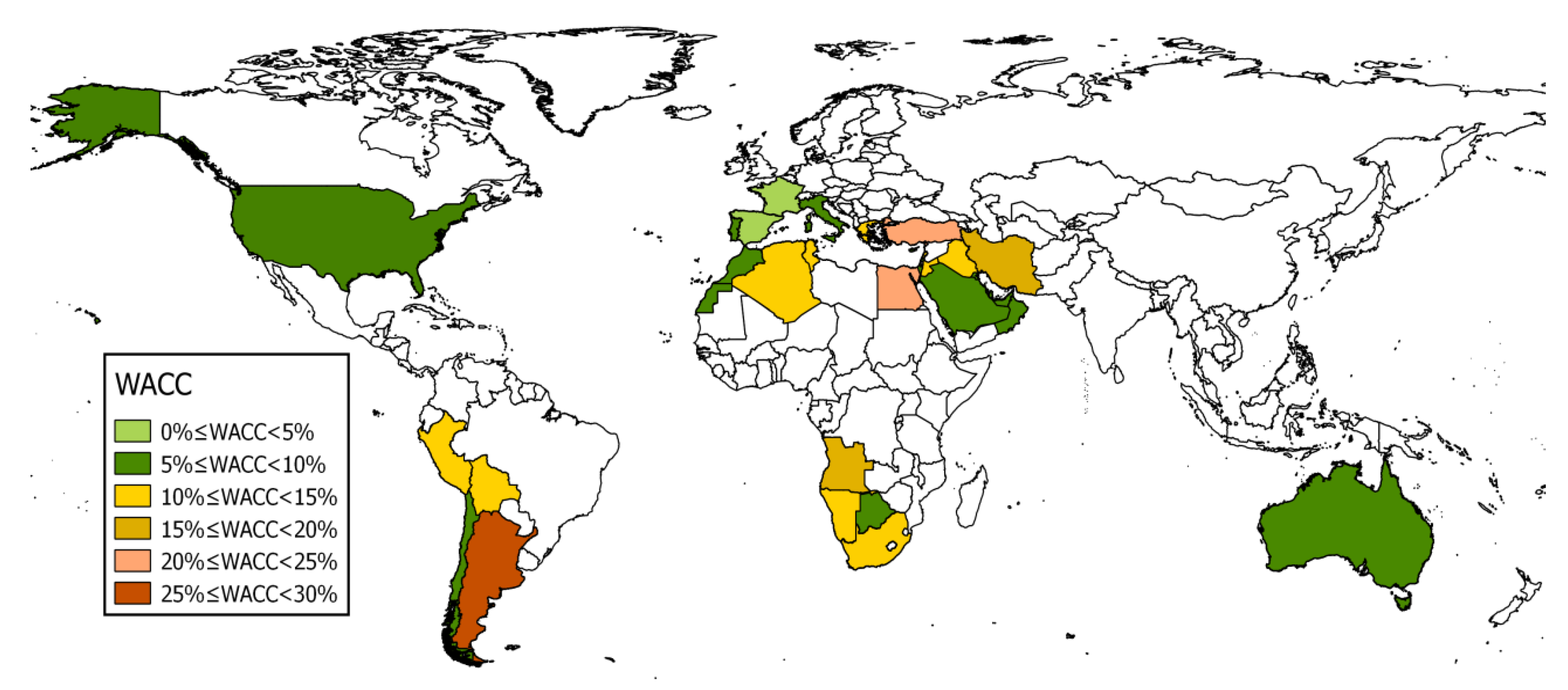
The data in Table 1 show that the costs of capital for a fuel production plant substantially vary across different countries. This is because some regions provide a more stable environment for investments than others, which is expressed in the interest rate estimates and inflation. High costs of capital represent the risk involved for the investor and thus increase the total costs of the investment. If interest rates and inflation are high, the resulting production costs of jet fuel will be high as well. This may render a very sunny location unfeasible for solar fuel production because of the resulting high costs of capital. An example is Egypt, which has the sunniest locations in the MED region but has very high interest rate estimates, which increase the production costs over those of Israel and even Spain, which have a smaller solar resource. This is also illustrated with an estimation of the weighted average costs of capital for the analyzed countries and the global DNI in Figure 2.

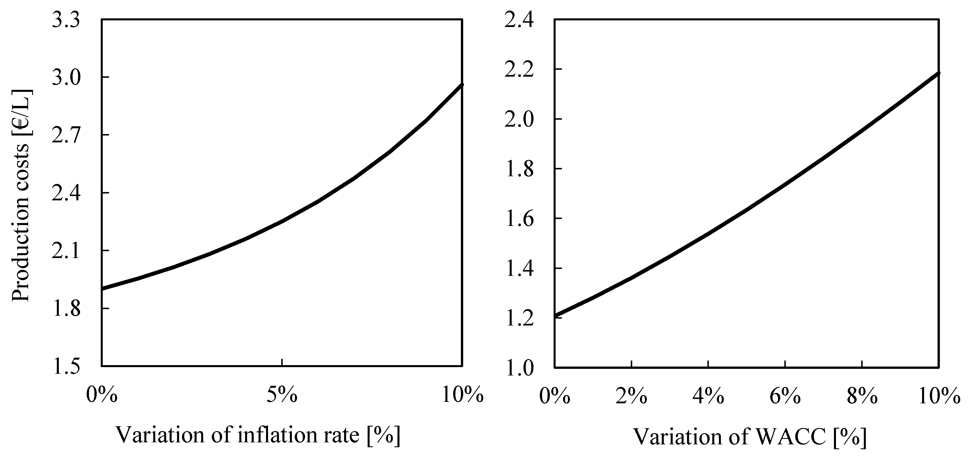
It is important to note that these estimated WACC were only a snapshot for the year 2017 and rely on aggregated proxy indicators. Thus, the cost of capital for a specific project in the future may be quite different from the estimates presented here. Our aim here is not to give a precise prediction of future investment environments, but to sensitize for the importance of country-specific variations in the cost of capital. The sensitivity of the production costs on the inflation rate and weighted average costs of capital is shown in Appendix A.5.

2.2.1. Investment Costs and O&M Costs

The investment and operating costs were estimated based on a model developed in [44] for a plant producing 1050 barrels per day (bpd) of jet fuel with naphtha as a by-product (see Appendix A.4. for a list of assumptions and costs). Naphtha is assumed to be sold at a relative price of 0.8 with respect to the production costs of jet fuel, corresponding to the correlation of market prices seen for conventional fuels [71,72]. The model is updated to include jet vacuum pumps instead of mechanical pumps and reforming of the light hydrocarbons produced in the FT reactor is performed. The use of vacuum pumps enabled significantly higher experimental efficiencies [7], where the costs for the pumps for this study are taken from [73]. The reforming of the light hydrocarbons enables a higher yield from the produced syngas. Furthermore, the thermochemical reactors and the gas-to-liquid conversion steps were modeled in more detail than in the previous publication using dedicated Matlab and Aspen models. CO₂ and H₂O are captured from the air based on chemical adsorption to an amine-functionalized solid sorbent [74] and are stored in tanks before being supplied to the thermochemical reactor operating at an efficiency of 19.0% (ratio of higher heating value of gases leaving the reactor to concentrated solar energy entering including auxiliary energy for heating the reacting gases) excluding the energy for vacuum pumping and gas separation. The specific cost of the air capture unit was assumed to be 350 €/t at fixed operational costs of 40 €/t, resulting in the long-term target costs of about 100 €/t [74]. The thermochemical reactors were assumed here to have a unit size of 50 kW at a cost of 14 €/kW each for the reactor shell excluding ceria, which does not preclude larger unit sizes. This cost estimate assumes a scaling exponent of 0.6 when scaling up from a single 50 kW-unit to the 2.8 GW of total thermal power of the current plant design, which corresponds to about 56,000 units of 50-kW reactors. The reactors complete 16 redox cycles per day using ceria as the reactive material, which is replaced after 500 completed cycles. This cyclability has been demonstrated in tests on a small material sample [75], while close to 300 cycles were achieved with a 4-kW reactor [6]. The efficiency of the reactors was assumed to be 19% in the baseline, which has not been achieved so far but is a realistic target for the development in the near to medium-term development. Taking into account the tower structure, the reactor shell and the reactive material ceria, the total cost of the receivers and tower is estimated to be 65 €/kW of thermal input power. This result assumes that the reactors can be mass-produced, achieving low production costs. The heat required in the reactor is supplied via the concentration of solar energy from a heliostat field with an aperture area of 8.8 million m² and the electricity with a dedicated CSP tower plant with a heliostat area of 0.57 million m². The size of the heliostat fields is dependent on the local DNI and thus changes with the location of the plant. A unit cost of 0.04 €/kWh_el was assumed for solar electricity, which is somewhat lower than the best-projected values of below 0.10 €/kWh_el from the newest CSP plants in China [76] and above the best values for PV electricity of 0.02 €/kWh_el [77,78] and could represent a future combined price of PV and CSP. The heliostat costs are set to 100 €/m², which is a likely cost value for the considered time frame of about 10–20 years in the future. Hydrogen and carbon monoxide coming from the reactor were stored and supplied to the Fischer–Tropsch (FT) plant, which has specific investment costs of 23,000 €/bpd and O&M costs of 4 € per barrel [79]. Light hydrocarbons from the FT unit are steam reformed and fed back into the FT process. The finished products were transported to the sea with a pipeline, which is assumed to be built for this purpose at specific costs of 90 €/m [80,81]. It is assumed that a direct connection to the sea from the plant location can be made and altitude differences in between are neglected. Final transportation of the products by ship over a distance of 1000 km is also taken into account at a unit cost of 0.8 cents per liter of liquid product [82].

For a plant of 1050 bpd, the jet fuel capacity located in a sunny region with a DNI of 2500 kWh/(m² y) and at a distance of 250 km to the sea, the total investment costs are 1.50 billion €. Of this sum, 59% are for the heliostat field, 8% for the thermochemical reactors, 7% for the CO₂ capture units and syngas storage, respectively, and other smaller contributions. The operational costs sum up to 55.2 million € per year, whereas the largest cost contributors are the heliostat field (32%), the capture of H₂O and CO₂ (21%), the generation of electricity (21%), and syngas storage (6%).

For plant operation and maintenance, a workforce is required with workers, technicians, engineers, management, and administration. To determine the number of direct jobs created, estimates of the total number of jobs in CSP plants are taken as a reference: the International Renewable Energy Agency (IRENA) estimates that 0.6–1.33 jobs are created per MW of the electrical output power of a CSP plant [83]. Sooriyaarachchi et al. analyze job creation in different renewable energy technologies and estimate 0.3 jobs per MWp [84]. In another publication of the IRENA, 0.2 jobs created per GWh are mentioned [85], while a report by Applied Analysis gives a number of 500–720 jobs per 2 GW plant [86]. The Energy Sector Management and Assistance Program (ESMAP) indicates 13–20 jobs created for a 500,000 m² solar trough power plant [87]. Finally, Solar Reserve published numbers regarding their newly built CSP plant in Port Augusta, Australia, mentioning 50 jobs for the plant of 135 MW [88]. These estimates, converted to the equivalent plant size of 2.8 GW thermal power (or 1.1 GW electrical power), give a corridor of about 200–500 jobs created for the baseline case plant with one larger estimate up to 1700 jobs. Using these figures as guidance, a total workforce of 396 is assumed, distributed into 246 workers, 100 technicians, 30 engineers, 15 clerks, and 5 managers. With data from the International Labor Organization (ILO) on annual salaries by occupation and country [89], the cost of labor is derived (see annex).

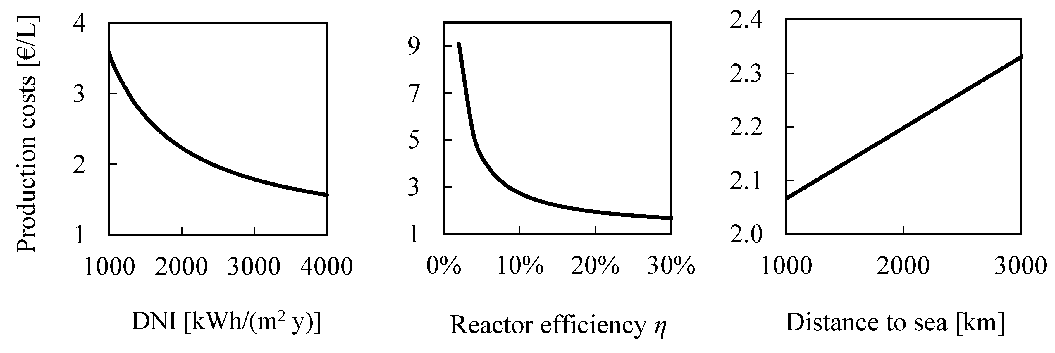
2.2.2. Dependency of Production Costs on DNI, Distance to Sea, and Reactor Efficiency

The production costs depend to a significant degree on the heliostat field, the size of which is determined by the DNI at the plant site and the reactor efficiency. At higher irradiation and a constant output of the plant, a smaller heliostat field can provide the required amount of concentrated energy to the solar reactors and thus the investment and O&M costs are decreased. At a less favorable site, the heliostat field may need to be enlarged to deliver the specified power, which will increase the production costs. The influence of reactor efficiency is like scaling the heliostat field and the associated costs. As a second geographical variable, the distance to the sea has an impact on the production costs because it determines the length of the pipeline for the distribution of the products. It is assumed that a direct connection to the sea can be made by the pipeline, neglecting altitude differences. At the sea, the products are then transported to their final location by ship over a distance of 1000 km. The dependency of production costs on DNI, distance from the sea and reactor efficiency is shown in Figure 3, whereas all other parameters are left constant.

From a DNI of 2000 kWh/(m² y), which was a value found in the South of Spain, to the best locations in the Andes at 3500 kWh/(m² y), the production costs dropped by about 25%. Equally, increasing reactor efficiency from 10% to 25%, the costs dropped by 35%. From a location directly at the sea to one that is 2000 km away from the shore, the production costs rose by about 15%. As a distance of 2000 km from the sea is found rarely, the DNI was very likely to have a stronger influence on the production costs. From the dependency of the production costs on these variables, a first conclusion can be drawn: an efficient reactor at a location with high solar irradiation located at or near the sea will reduce production costs under otherwise constant conditions.

3. Results

Using the methodology described above, the suitable areas in the regions of the Mediterranean region (MED), the USA, South America, South Africa, and Australia are identified. Having identified the suitable areas, the production volumes and production costs are determined.

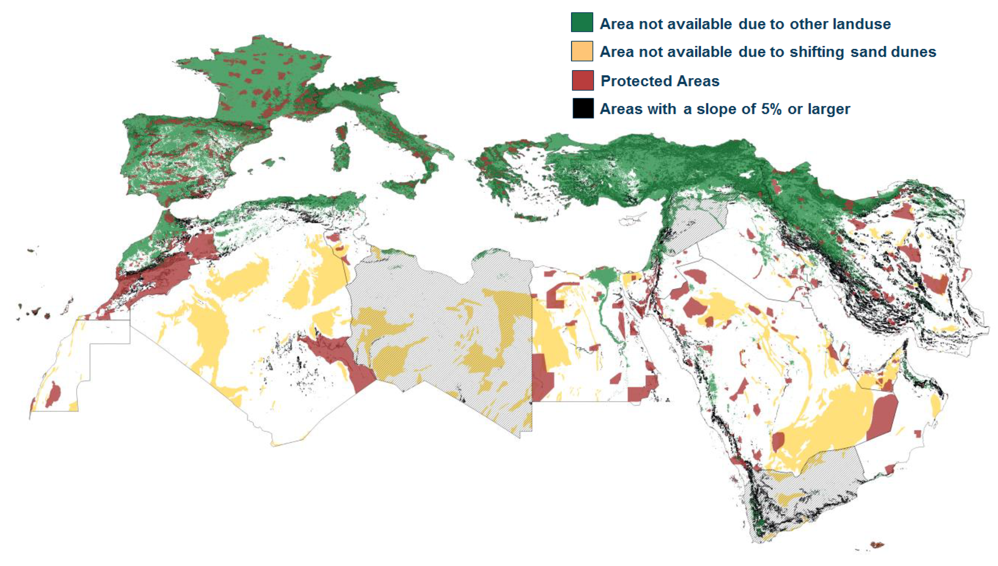
3.1. Suitable Areas for Solar Thermochemical Fuel Production

In the following maps, the exclusion of areas is indicated with colors (green: land use, red: protected areas, yellow: shifting sand dunes, black: slope ≥5%), while the suitable areas within national boundaries are shown in white.

The excluded and suitable areas in the MED region are shown in Figure 4. In Europe, only very little area is available due to other land uses such as agriculture and livestock farming, and due to large areas being protected from other uses. Suitable areas are mostly found in Spain and Turkey. In northern Africa and the Arabian Peninsula, there are vast suitable desert areas where the climate is too dry for agricultural use. Excluded areas are found in Morocco and throughout the other countries in northern Africa and the Middle East mostly due to shifting sands and protected areas. Agricultural areas are found mostly along the shore in Morocco and Algeria, along the river Nile, and on the eastern Mediterranean coast.

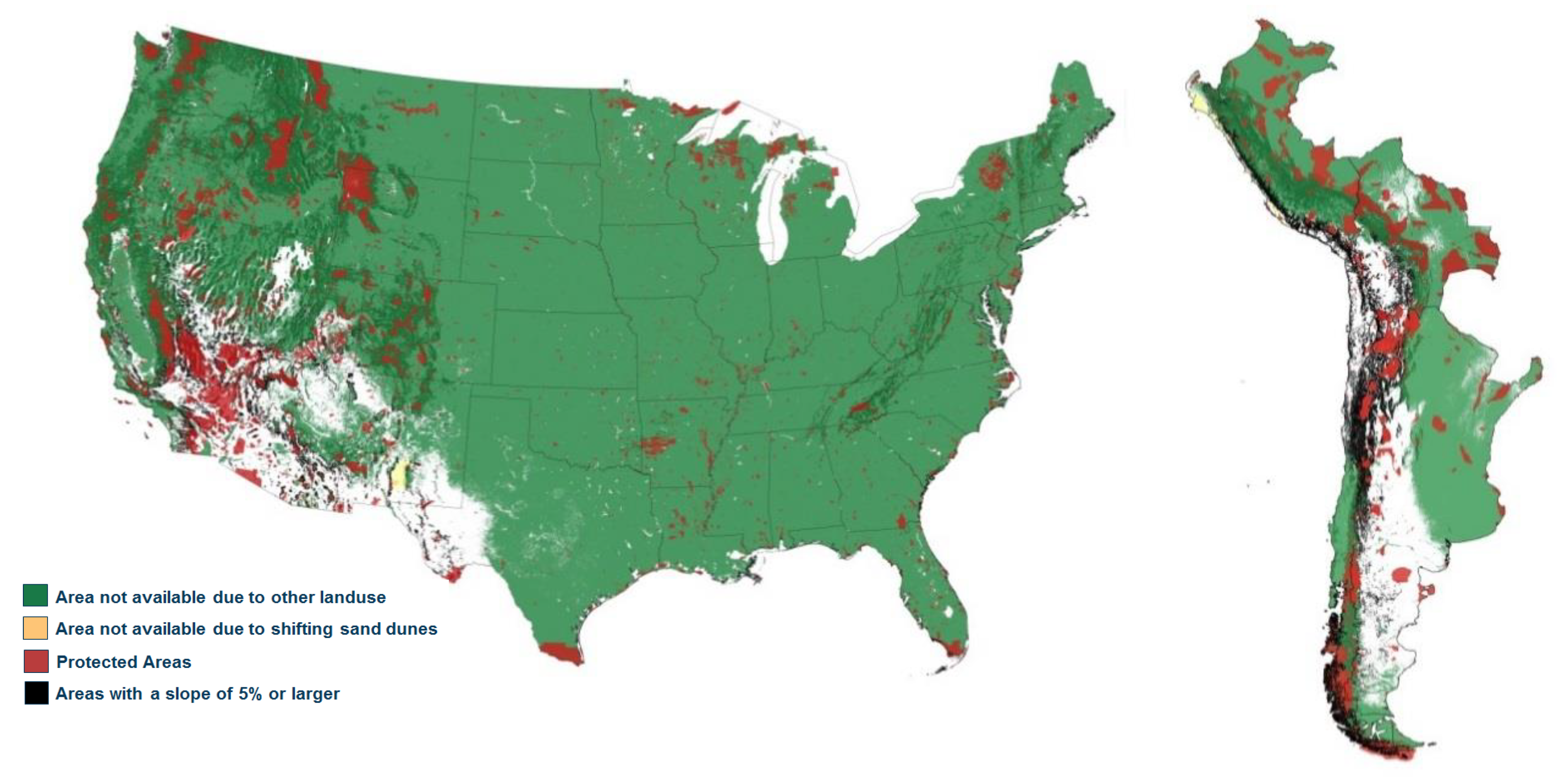
In the USA (Figure 5), most of the land is being used for agriculture and livestock farming or is protected in national parks. In the Appalachian and Rocky Mountain regions, the terrain may be too steep for the construction of a fuel production plant. The suitable areas are found in the southwest, where the solar irradiation is also highest. While most of the country is unavailable for solar thermochemical fuel production, the remaining suitable areas are nevertheless considerable in size and could enable large fuel production. In South America (Figure 5), the most favorable locations are found in the Andes region due to the particularly high DNI in the desert at high altitudes. Due to the mountainous region, however, many locations have too steep slopes to be used for the construction of a plant. Large regions are also excluded due to site protection, agriculture, and livestock farming, leaving the largest suitable areas in eastern Argentina. 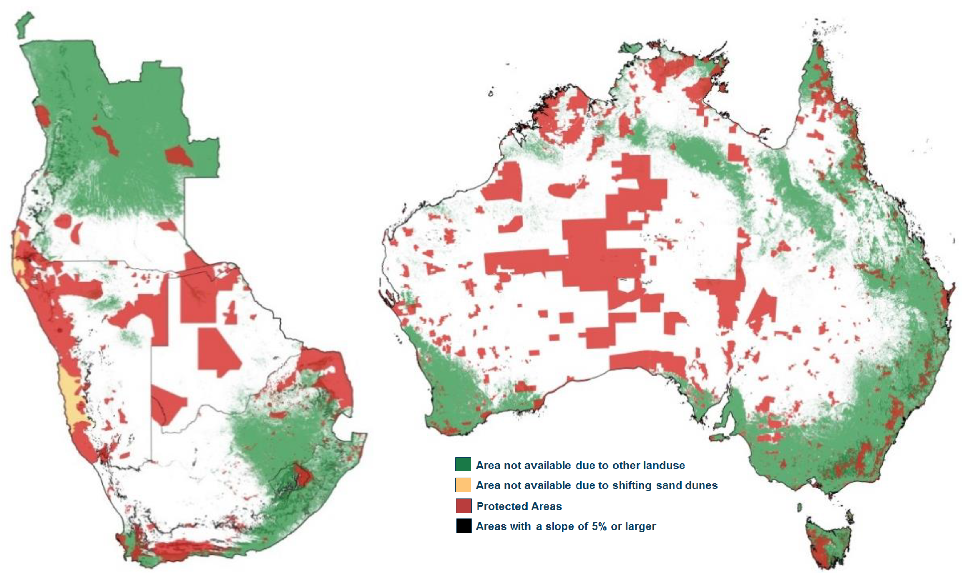In the eastern part of South Africa (Figure 6) mainly grassland and cropland prohibit the production of solar fuels. In the northern part of Angola, the land is covered mainly by woody savannas, evergreen broadleaf forest, and cropland at the coast. There are also a number of protected areas such as the Kruger national park or the Kalahari Desert, which are excluded, as well as shifting sands along the coast in Namibia and Angola. Nevertheless, there remain large connected areas in all four countries that are theoretically available. In Australia’s (Figure 6), southeast, cropland and evergreen broadleaf forest, and protected areas all over the country significantly reduce the available areas, which are however still the largest found in a single country.

3.2. Production Potential on Suitable Areas

After the identification of suitable areas, it is possible to derive the production potential of solar thermochemical fuels. For this purpose, a conversion factor is defined that expresses the fraction of DNI that is turned into jet fuel. This conversion factor is comprised of the energy conversion efficiency of the fuel production process and the land-use factor, whereas the latter is the area of the heliostats divided by the area of the land, and which is assumed to be 25% [90]. The energy conversion efficiency of direct solar irradiation to jet fuel is 2.46% (based on updated calculations of [44], see Appendix A.3 for more information), where naphtha is produced as a by-product. The conversion factor is then 0.25 × 0.0246 = 0.61%. Thus, at a common annual DNI of 2500 kWh/(m² y), 2500 kWh/(m² y) × 3.6 MJ/kWh × 0.61%/33.4 MJ/L = 1.66 L of jet fuel are produced per square meter and year. For the calculations of the production potential, it is assumed that the conversion factor is constant and thus independent of the DNI. In

Table 2. Calculated suitable areas and production potential of solar thermochemical fuels in different regions.

	Suitable Area for Solar Fuel Production [106 km2]	Suitable Area/Calculated Country Area [%]	Production Volume on Suitable Areas [103 Mt/y] b	Production Volume/World Demand [-]
MED region	5.71	52	6.13	20.4
Australia	4.49	59	5.81	19.4
South Africa, Botswana, Namibia, Angola	1.87	48	2.38	7.9
Chile, Argentina, Peru, Bolivia a	1.24	23	1.47	4.9
USA a	0.599	8	0.777	2.6

^a The deviation from the FAO area is largely due to the data being restricted to latitudes between 60° N and 45° S. ^b Current global jet fuel consumption is about 300 Mt/y [91].

the sum of the areas suitable for fuel production is shown for different regions of the earth together with the production volumes of solar fuels.

In the Appendix A (

Table A1. Suitable areas and production potential for each country.

Region or country	Calculated Country Area/FAO Area a [%]	Suitable Area for Solar Fuel Production [km2]	Suitable Areas/Calculated Country Area [%]	Production Volume on Suitable Areas [t/y] b
MED region	97%	5,708,154	52%	6.13 × 109
Algeria	97%	1,634,220	71%	1.77 × 109
United Arab Emirates	98%	22,169	32%	2.17 × 107
Egypt	98%	623,294	64%	7.30 × 108
Western Sahara	100%	234,366	88%	2.58 × 108
Spain	101%	90,350	18%	9.02 × 107
France	99%	301	0%	2.41 × 105
Greece	96%	1141	1%	1.01 × 106
Iran	99%	852,589	53%	8.50 × 108
Iraq	102%	371,169	84%	3.62 × 108
Israel	100%	8410	39%	1.01 × 107
Italy	100%	3571	1%	3.01 × 106
Jordan	100%	76,434	86%	9.88 × 107
Kuwait	93%	12,818	78%	1.23 × 107
Lebanon	98%	1625	16%	1.90 × 106
Morocco	92%	109,033	26%	1.19 × 108
Oman	100%	267,654	87%	2.88 × 108
Portugal	99%	9258	10%	9.15 × 106
Qatar	97%	8147	73%	7.75 × 106
Saudi Arabia	89%	1,234,473	65%	1.35 × 109
Tunisia	99%	95,635	62%	9.75 × 107
Turkey	100%	51,497	7%	5.16 × 107
Southern Africa	100%	1,865,708	48%	2.38 × 109
South Africa	100%	638,011	52%	8.51 × 108
Namibia	100%	479,794	58%	6.61 × 108
Botswana	102%	402,197	70%	4.91 × 108
Angola	100%	345,706	28%	3.78 × 108
South America	92%	1,236,859	23%	1.47 × 109
Argentina	90	827,786	34%	9.32 × 108
Bolivia	100	210,907	19%	2.58 × 108
Chile	70	135,695	26%	2.12 × 108
Peru	101	62,471	5%	6.88 × 107
Australia	100%	4,487,022	59%	5.81 × 109
USA	84%	599,503	8%	7.77 × 108

a. Area as determined by the Food and Agriculture Organization of the United Nations (www.fao.org); b. Jet fuel; not counting the by-product naphtha.

), the calculated total areas of the countries in the different regions are compared with the areas indicated by the FAO [92] to test the calculation methodology of the geographic information system. The largest suitable areas for solar fuel production are found in the MED region with close to 6 million km², where the largest areas (≥10⁶ km²) are found in North Africa and the Middle East, i.e., in Algeria, Western Sahara, and in Saudi Arabia. As a single country, Australia has by far the largest potential with about 4.5 million km² of suitable area corresponding to more than half of the country area. In the MED region, the share of suitable areas in the respective country areas is also high with >50% on average, whereas this value is mainly achieved in North Africa and the Middle East, where large regions are available in the desert. The value found for the countries in southern Africa is also close to 50%. In the USA, however, below 10% of the country is suitable for solar fuel production, which is due to large areas being used for agriculture and farming. The suitable and most interesting sites are found in California, Nevada, Arizona, New Mexico, and Texas, which is where the solar irradiation is highest. For comparison, the SunShot study found suitable areas of about 0.226 × 10⁶ km² in the Southwest of the US with more stringent exclusion criteria for slope and a lower bound for the DNI [68], while another study found 0.985 × 10⁶ km² [14]. The potential found in this study is in between these values, where the differences stem from the definition of the exclusion criteria. In the analyzed countries in South America, only about 20% of the total areas are found to be suitable, which is mainly due to high slopes in the Andes region, agricultural land use, pastureland, and protected areas.

The volume of fuel that can be produced on a given area can be derived by multiplying the area by the specific productivity, which is dependent on the local solar irradiation. In Table 2, the sum of the production volumes that could be achieved on the suitable areas in the chosen regions is shown. The largest volumes can be produced in the MED region due to the largest available areas and quite high DNI values in the Sahara Desert and on the Arabian Peninsula, whereas the highest DNI is found on the Sinai Peninsula in Egypt. The production volumes reach 6.1 × 10³ Mt/y, which is more than 20 times the current value of global jet fuel consumption (about 300 Mt/y [91]). The other regions achieve smaller production volumes of about 5.8 × 10³ Mt/y in Australia, 1.5 × 10³ Mt/y in southern America, 2.4 × 10⁶ Mt/y in southern Africa, and 0.8 × 10³ Mt/y in the USA, which is still more than twice the global jet fuel consumption. Therefore, all areas and even single countries are in principle capable of producing enough jet fuel to cover the current global demand, which means that almost all countries (except France) are able to cover their own demand to become independent of oil imports for aviation and possibly also for other transport sectors. With this huge potential for fuel production, it is possible to limit the choice of areas to the best locations with the lowest production cost.

3.3. Life-Cycle Production Costs of Solar Thermochemical Jet Fuel

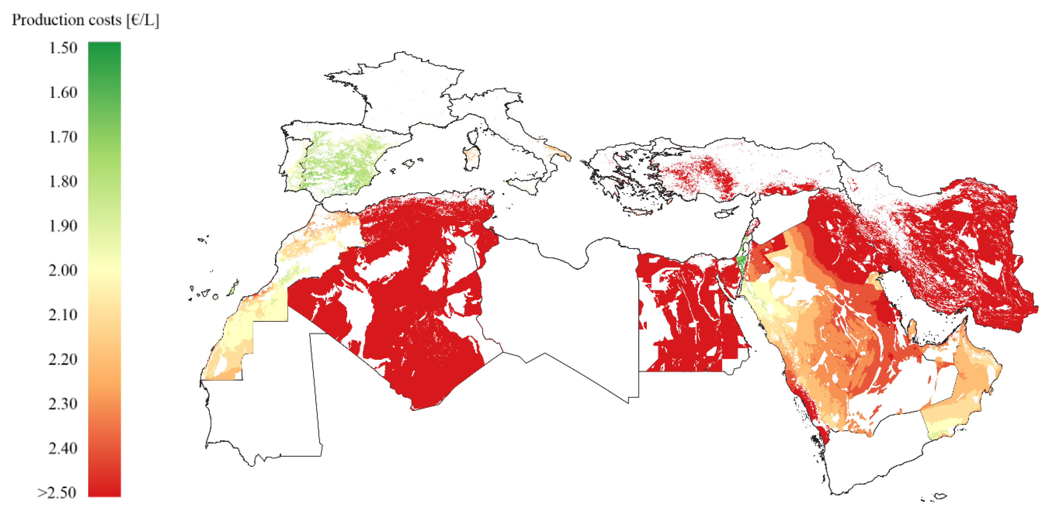
In the following, the production costs of solar thermochemical jet fuel are analyzed in the most interesting regions. The results are displayed as cost-supply curves, i.e., production costs per liter are shown as a function of the respective amount of fuel that can be produced at that cost. For production costs maps of the regions, please refer to Appendix A.2. 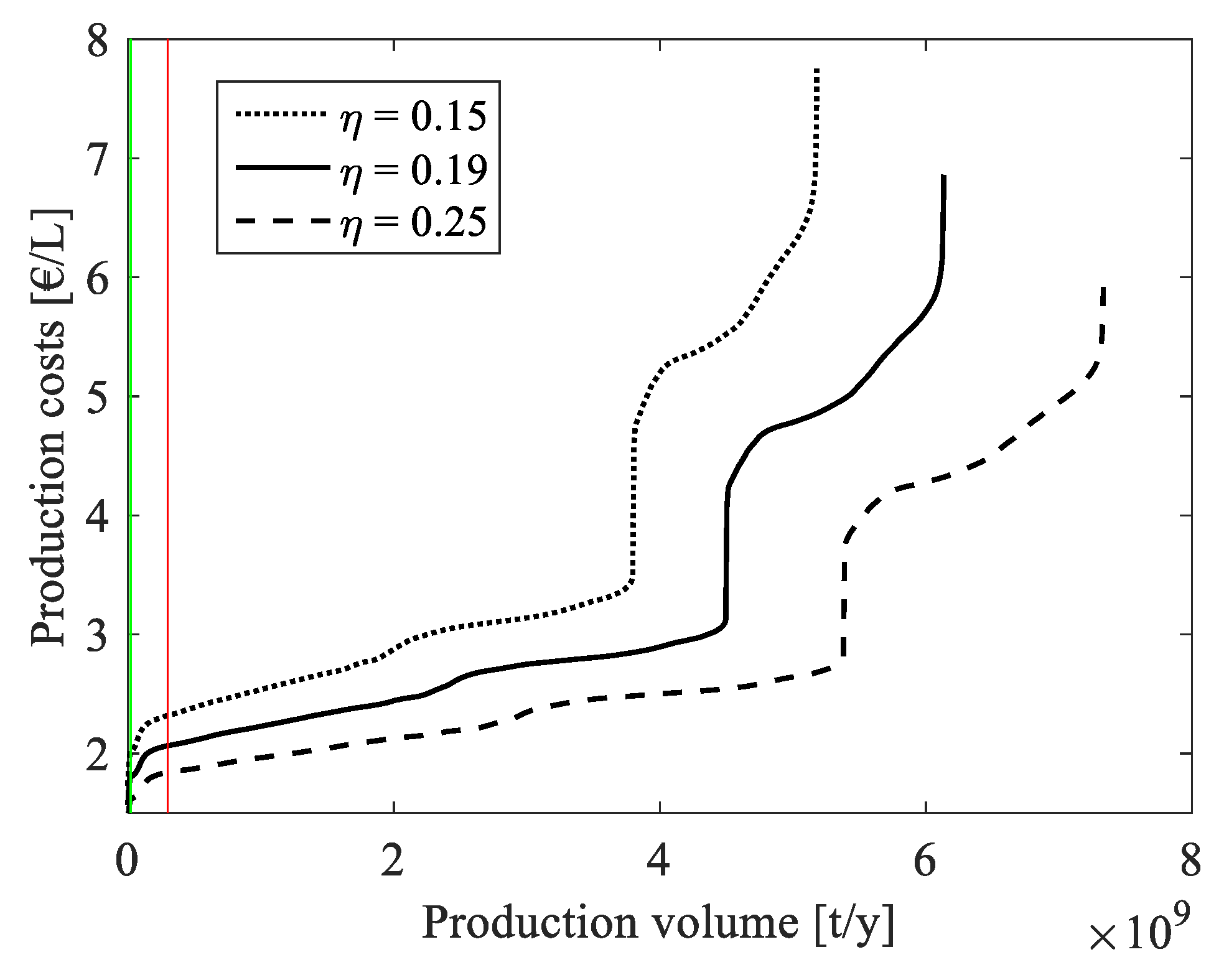To facilitate the analysis of the production volumes, the current jet fuel consumption (2015–2017, depending on data availability [93], green line in the graphs) in the selected regions is given and also the global jet fuel consumption [91] of 300 Mt/y (red line in the graphs). As the fuel production potential exceeds the world demand in all of the analyzed regions, the graphs are limited to supply up to the world demand and the region of the graphs beyond the world demand are shown only in the Appendix A.1. for completeness.

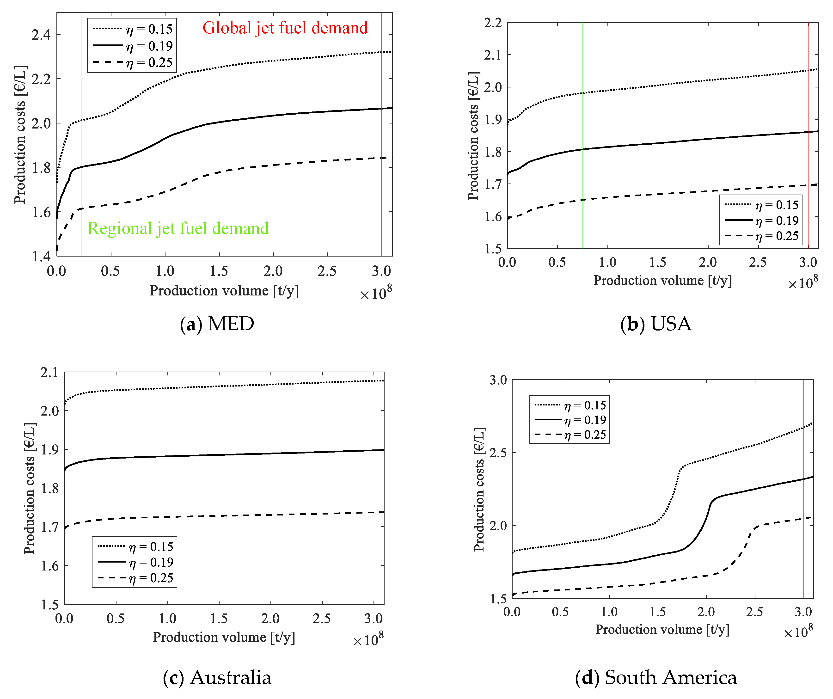
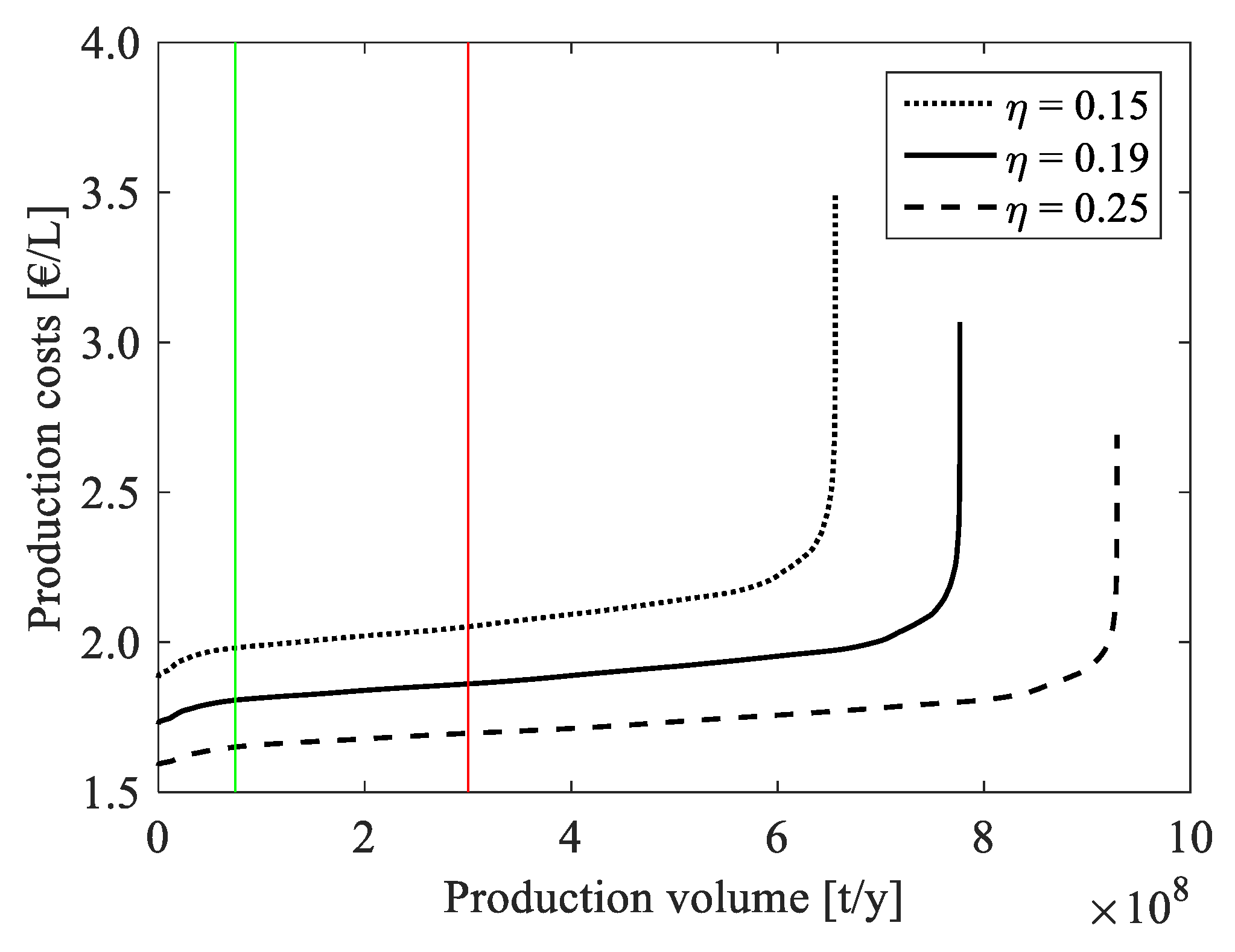
In Figure 7, cost-supply curves for the selected regions are shown for reactor efficiencies of 0.15, 0.19, and 0.25. In general, the change in efficiency leads to a shift of the cost-supply curves, where a higher efficiency reduces the costs due to the smaller heliostat field required. Among the interesting process parameters, reactor efficiency has been chosen to be varied here due to its large influence on costs and its large potential improvement over the current state of the art. In the following, the results are discussed only for the case of a reactor efficiency of 0.19. In the MED region (Southern Europe, northern Africa and the Middle East), there is a large production potential for solar fuels, which easily exceeds the global jet fuel demand (see Appendix A.1 for full curves). The curve indicates that the local jet fuel demand could be covered with production costs between 1.58 and 1.82 €/L, with average costs of 1.75 €/L, and the global demand at costs of 1.58–2.09 €/L (average 1.98 €/L). The lowest production costs are found in regions with high solar irradiation and favorable financial boundary conditions (interest rate estimates and inflation), i.e., in Israel and Spain, while the highest DNI occurs in Egypt and in Saudi Arabia. However, in the latter countries, the cost of capital is comparably high, which leads to overall higher production costs. It should be noted that the chosen economic model is based on the assumption of market conditions for the cost of capital and does not take into account other political boundary conditions such as purchase agreements or financial support.

The curve thus starts at the lowest costs in the most favorable production locations of Israel and Spain and further includes mainly Morocco, Western Sahara, and Saudi Arabia. The inclination of the cost-supply curve indicates the availability of areas on which fuel can be produced at the specific costs. A steep curve section thus represents a comparably restricted supply capability, which is due to the limited areas available at the respective irradiation and financial conditions. A flat curve section, on the other hand, indicates that large amounts of fuel can be produced at rather constant production costs.

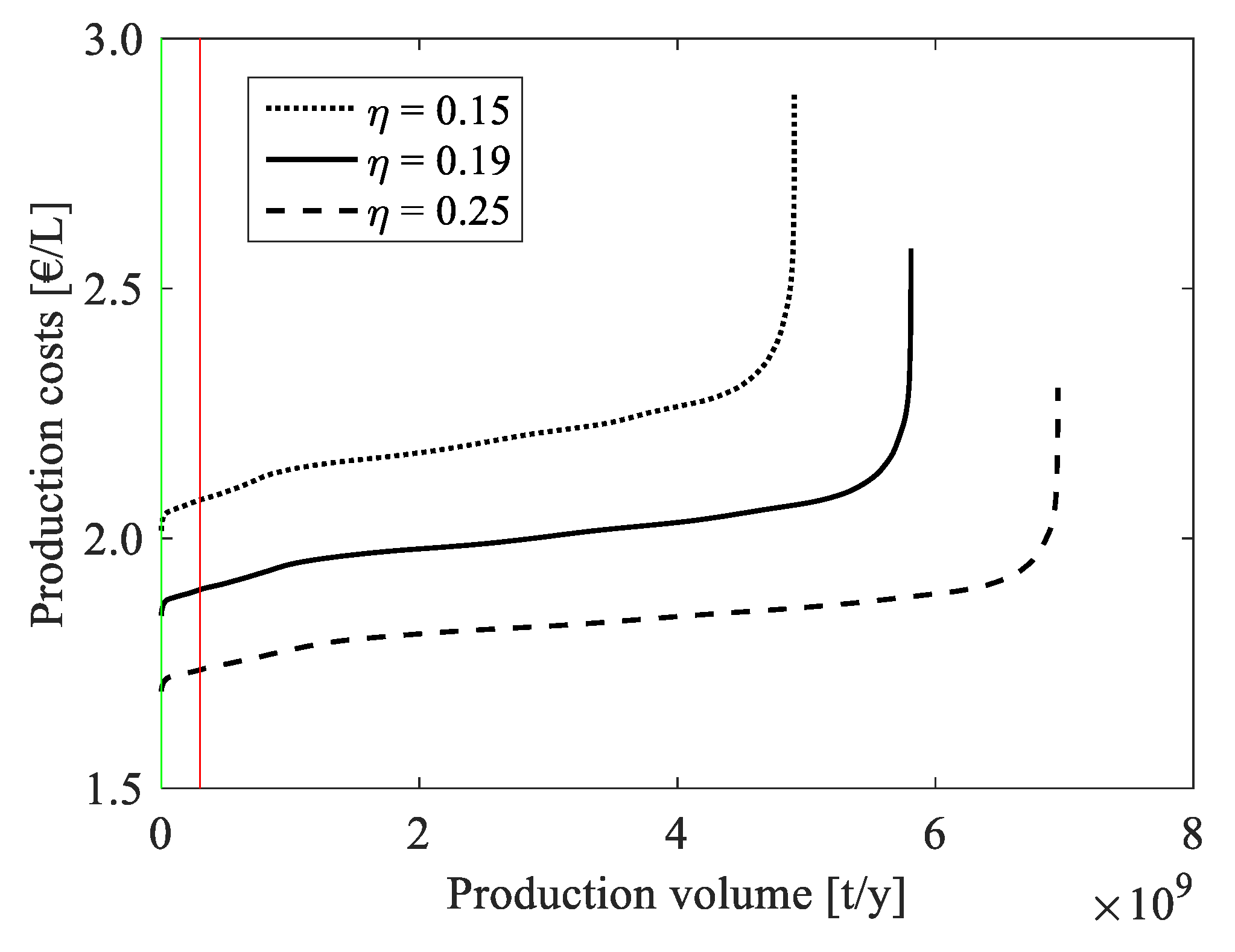
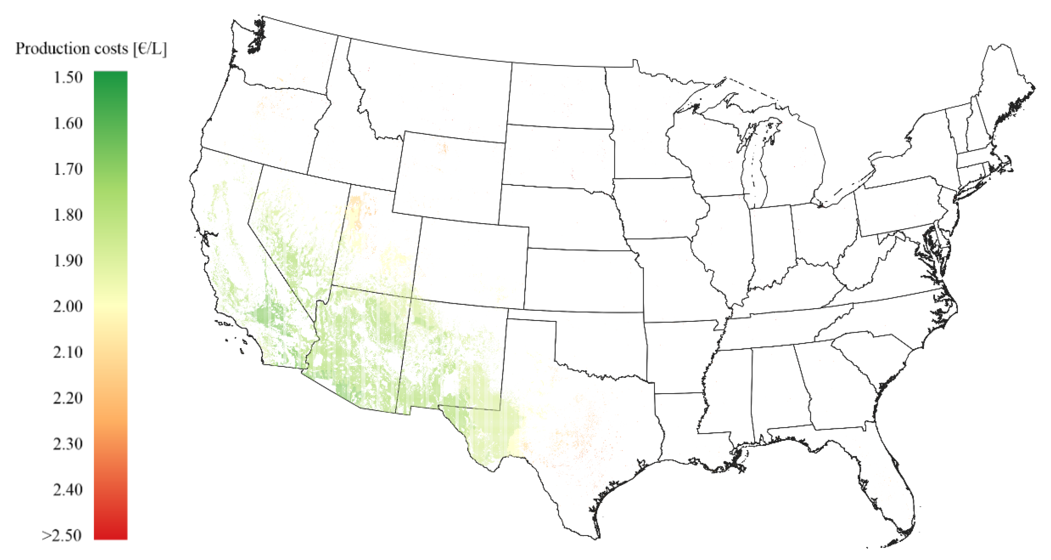
The USA has quite highly irradiated areas in the southwest and very favorable costs of capital, enabling low-cost production of solar fuels. At the best locations, production costs of under 1.75 €/L can be achieved, whereas the national demand for jet fuel could be covered at costs between 1.74 and 1.82 €/L, and at average costs of 1.79 €/L (Figure 7b). If the global jet fuel demand were to be covered, the costs would be between 1.74 and 1.88 €/L at average costs of 1.84 €/L.

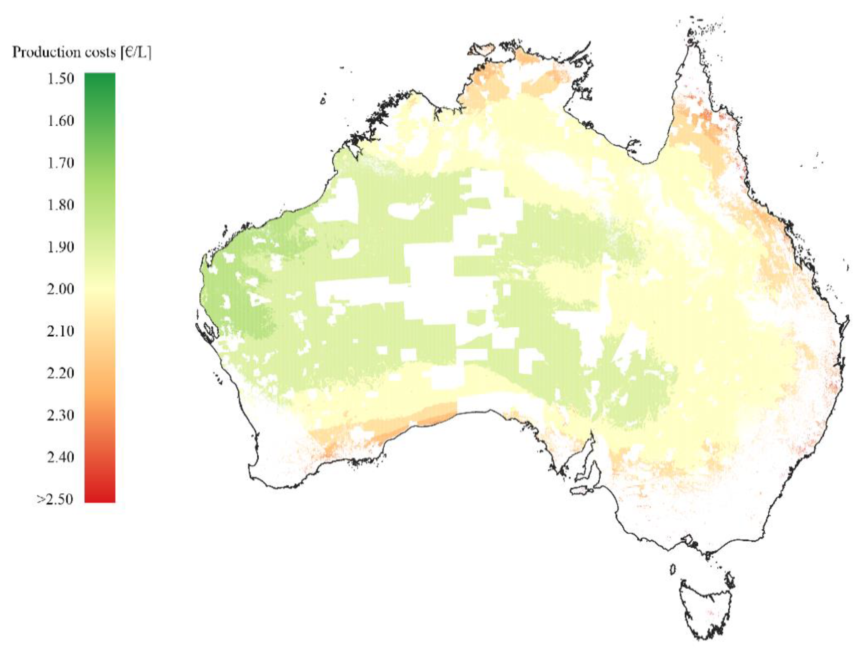
In Australia, very large areas with high solar irradiation are suitable for solar fuel production, which leads to the highest production potential of a single country. The national and global demand of jet fuel can therefore easily be covered with a fraction of the available areas at costs of 1.86 €/L for the former and between 1.86 and 1.91 €/L for the latter at an average of 1.90 €/L. The best locations are found in the northwest, where the highest values of solar irradiation are found and the distance to the sea is short. Somewhat higher costs of capital and labor costs in Australia prevent even lower production costs. If the financial boundary conditions could be further improved, the country could become a very favorable location for the production of solar fuels.

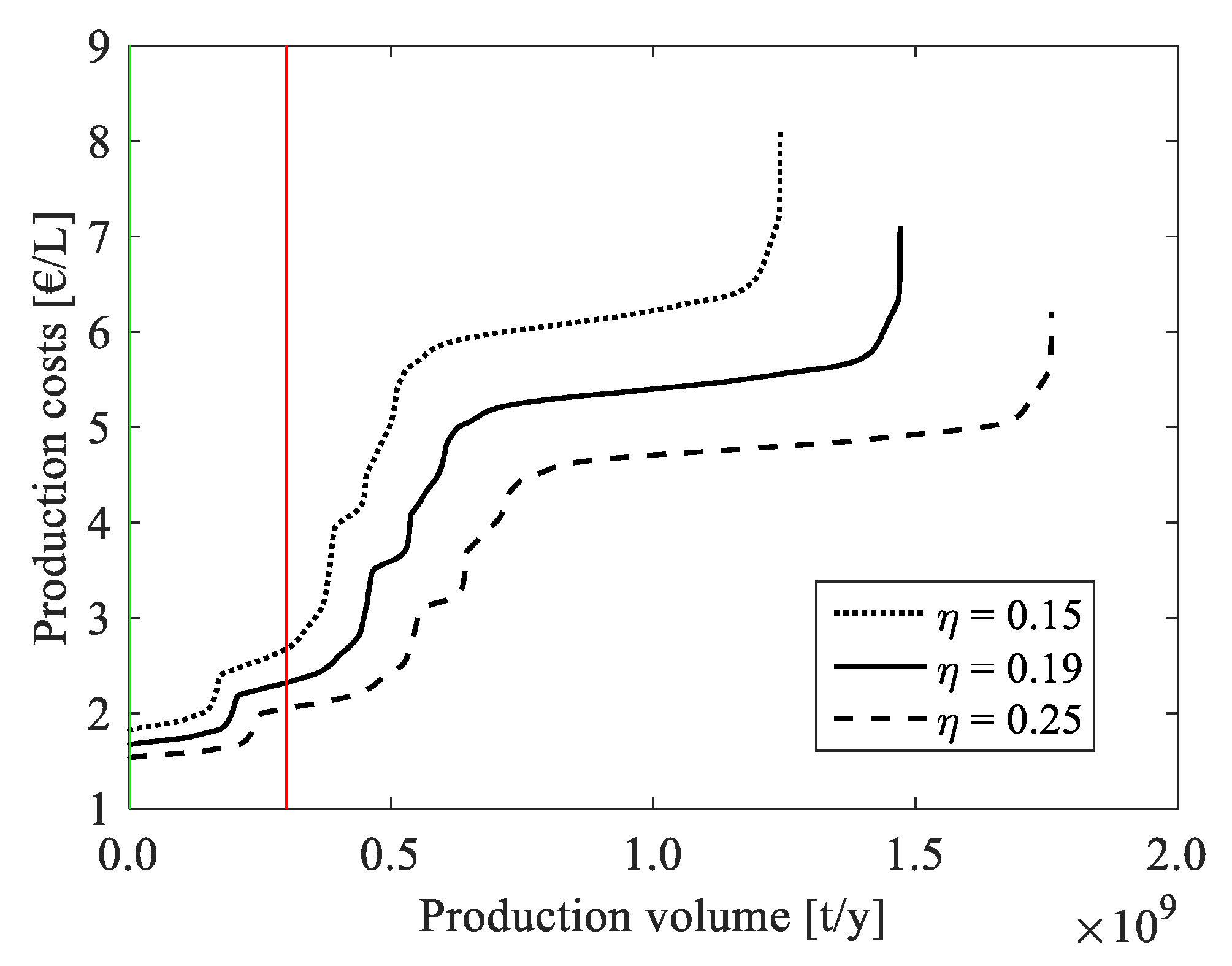
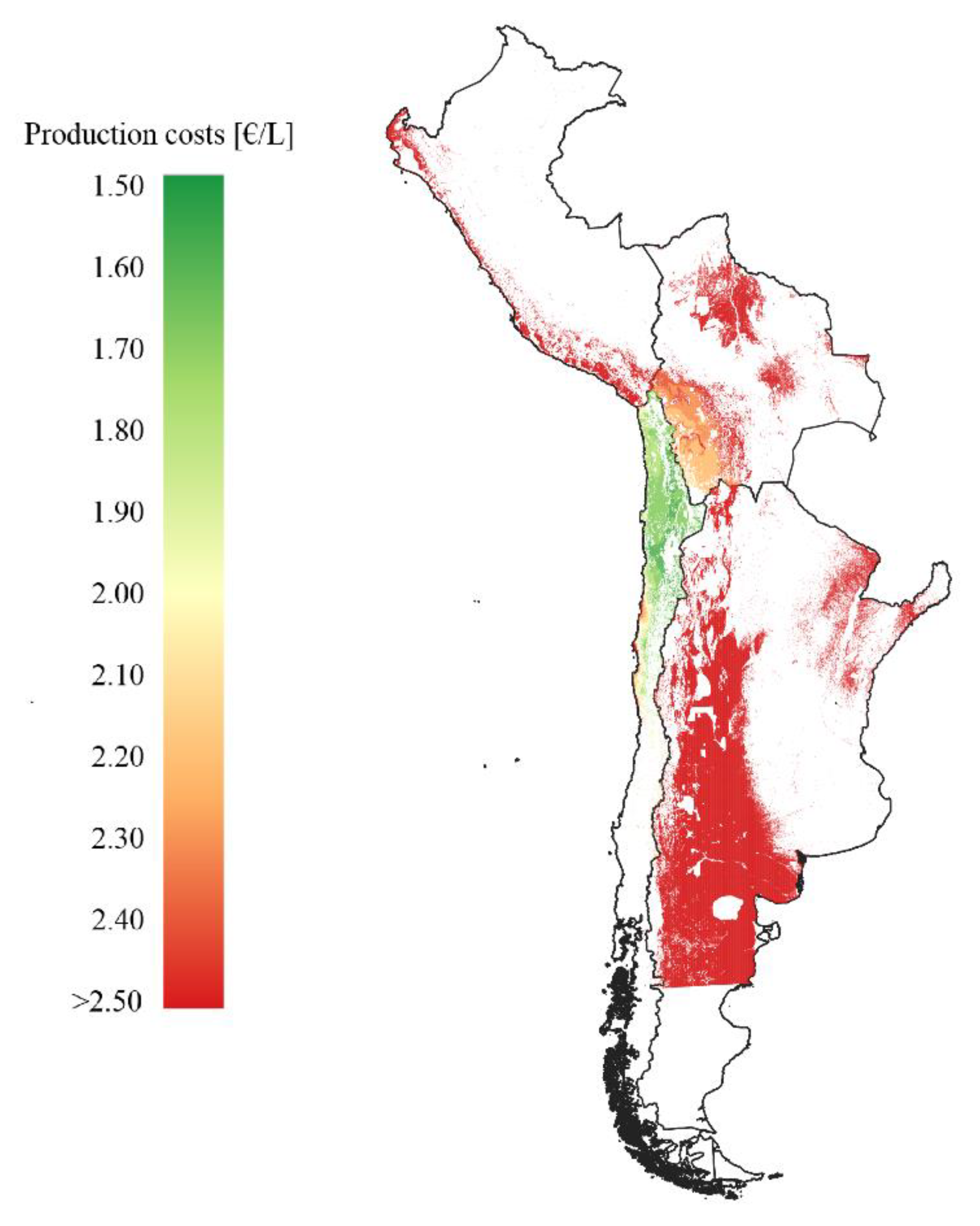
The South American Andes region is an excellent location for the conversion of solar energy with the highest values of direct solar irradiation found globally. From a technical point of view, this region is therefore ideally suited for solar fuel production with maximum DNI values exceeding 3500 kWh/(m² y). On the other hand, the regional financial preconditions are somewhat less favorable with relatively high estimates of interest rates: the weighted average cost of capital is between 7.1% in Chile and 29.3% in Argentina. The resulting production costs thus rise to higher values than in the best locations of the MED region with DNI values of about 2700 kWh/(m² y) in Israel with a WACC of 5.3%. Nevertheless, Chile offers exceptionally good conditions for the production of solar fuels, which enable production costs below 1.67 €/L. The regional demand of the selected countries can be covered at average costs of 1.68 €/L and the global demand at 1.67–2.34 €/L (average: 1.94 €/L). In the graph, the production locations are found only in Chile and Bolivia due to their favorable conditions. The production costs rise slowly from low values in Chile and experience a sharp rise when the least favorable production locations in Chile are selected. At an accumulated production volume of about 2.25 × 10⁸ t/y, the production moves into Bolivia, which has higher production costs than Chile according to its higher cost of capital (nominal WACC: 11.8%). The slope of the production costs rises again slowly up to the production volume in Bolivia corresponding to the global demand.

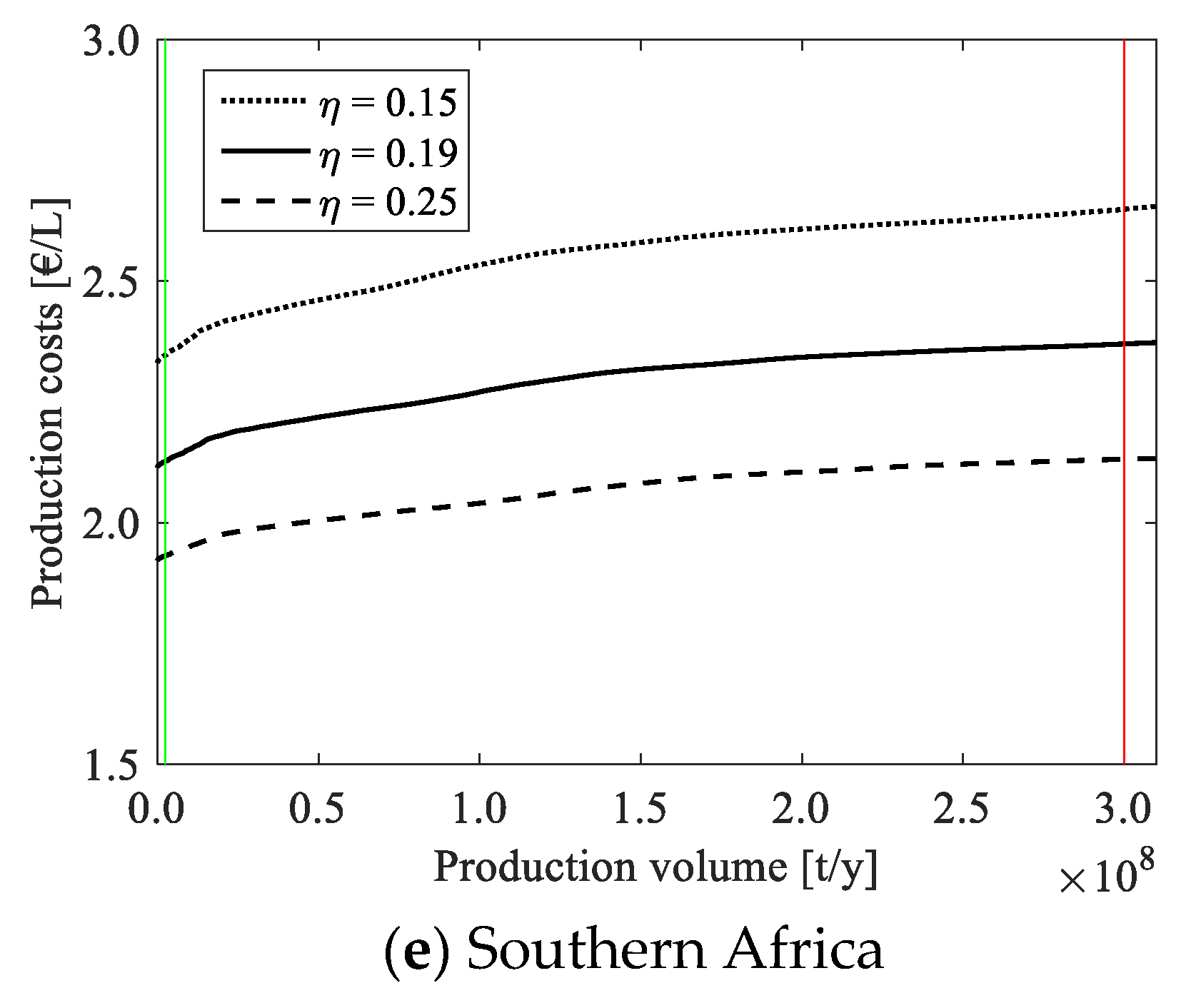
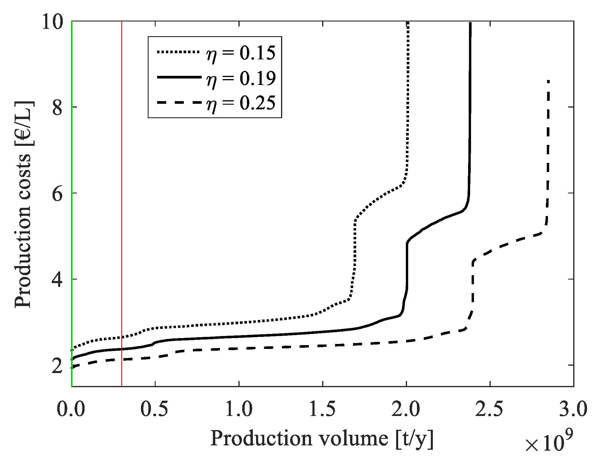
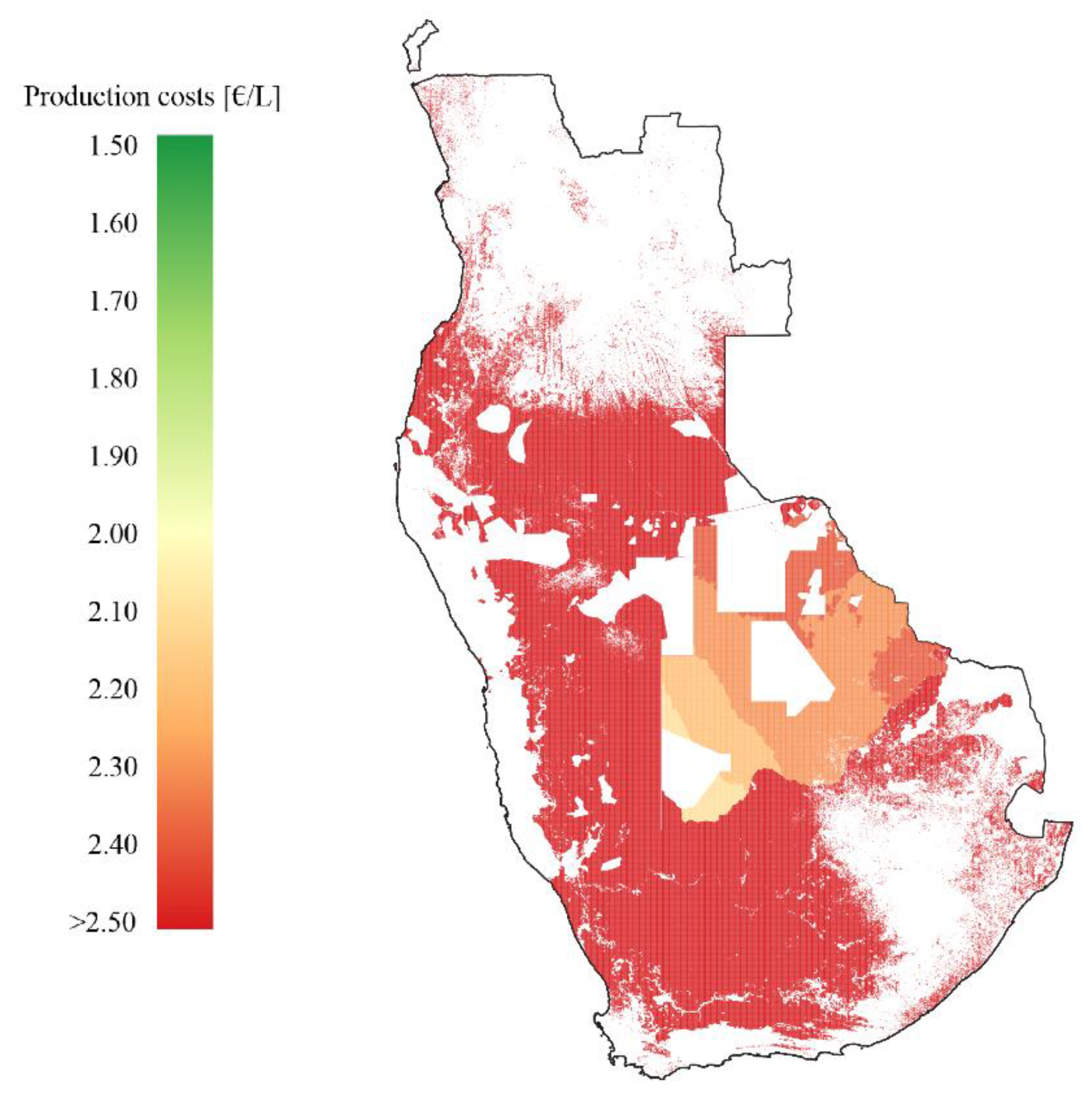
In southern Africa, the solar irradiation is also relatively high, making this region likewise favorable from a technical point of view. The production potential is quite high, exceeding those for the selected countries in South America. However, the cost of capital is comparably high with the lowest nominal WACC found in Botswana at 8.8%, about 13% in South Africa and Namibia, and up to 18.4% in Angola. The resulting production costs start at 2.13 €/L in Botswana, whereas locations in Namibia and South Africa have the lowest costs of 2.51 €/L and 2.53 €/L, respectively. Angola has very high costs of capital, preventing the production of solar jet fuel below 4.8 €/L. In southern Africa, the regional demand could, therefore, be covered at average costs of 2.14 €/L and the global demand at 2.32 €/L using the best locations found in Botswana.

In general, the flat progression of the cost-supply curve suggests that large-scale production of solar fuels could be set in place at relatively constant production costs. For the sake of clarity and simplicity, we do not conceptualize a dynamic cost model, which incorporates decreasing production costs with increasing production capacities. Thus, more sophisticated models could incorporate economies of scale and learning effects to better capture cost dynamics with increasing capacities. Note that a precondition for its deployment on a GW-scale is the availability of all technologies at a high technology readiness level (TRL). While still at lower TRL today, the current development of CO₂ air capture and reactor technology is promising [7,27]. At a GW-scale, the availability of ceria could provide a challenge and require its replacement with other available and tested reactive materials such as perovskites [40].

4. Discussion

In the preceding analysis, the cost of capital was geographically varied by modeling the local interest rates for debt and equity and using country-specific inflation rates. This leads to differing WACC estimates in each state. Under otherwise constant conditions, the production costs of solar jet fuel will be higher in a country with high costs of capital (i.e., a high WACC) than in a country with a low WACC. A deviation from this behavior may occur for locations with differing geophysical and macroeconomic conditions, e.g., different levels of solar irradiation and thus sizes of heliostat fields, or for countries with deviating inflation rates. The results shown above, therefore, reflect a change in estimated investment costs, in WACC, and inflation rates across countries. Besides these varying costs of capital, it is interesting to look at the case of constant nominal WACC across countries to analyze the effect on the cheapest production locations of solar jet fuel. This represents the case where e.g., the state acts as a guarantor for the investment into the fuel plant and thus enables a low cost of capital. In the following the nominal WACC is—hypothetically—held constant across countries at a level of 4% or 10%, respectively. The inflation rates are, however, still country-specific and are much harder to influence by governments. This is due to the fact that inflation is influenced by a variety of macroeconomic dynamics, and that central banks—the institution with the strongest means to influence inflation—often act independently from governments. This results in constant nominal WACC values but varying real WACC values across the locations. Note that locations with high inflation rates then show lower production costs. This counterintuitive result can be explained by the guaranteed nominal interest rates, which result in lower real interest rates at higher inflation. In other words, if the state finances investment projects at a certain nominal cost of capital (e.g., in countries with relatively high-interest rates), it will have to refinance itself through government bonds to a real interest rate, which is likely higher than the guaranteed nominal cost of capital.

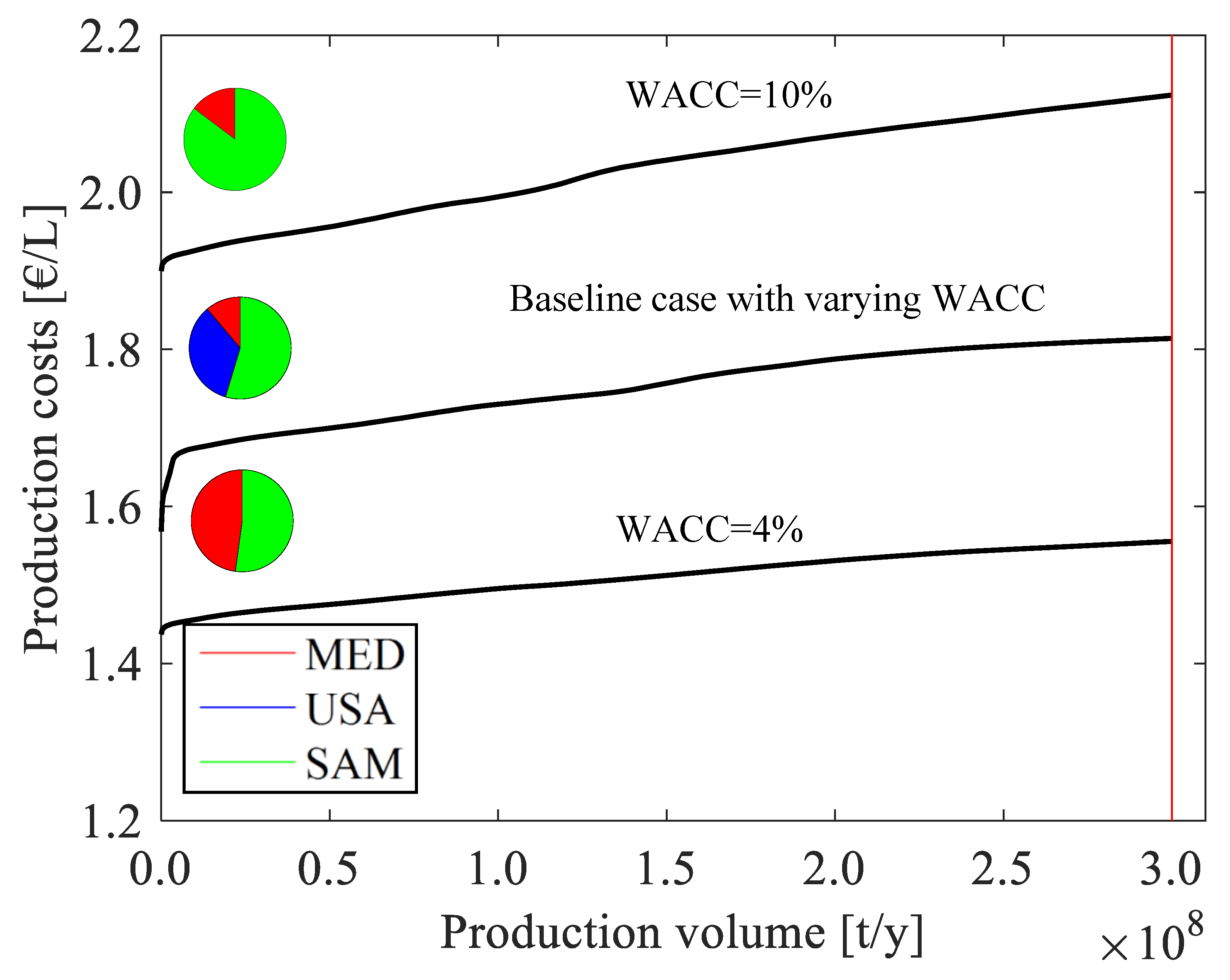
It should be noted that a fluctuation in exchange rates could lead to partial compensation of this development. In other words, countries with high inflation rates could see their currency depreciate over time, which reduces the prices of domestically produced goods on global markets. However, as exchange rates do not only depend on the inflation rates in different countries, a quantification of this effect is rather difficult and out of the scope of this paper. In most countries, the inflation rate is between 0% and 5%, while in some cases it can reach 10% and above (i.e., in Egypt, Angola, and Iran). This should be kept in mind when interpreting the following results. The resulting cost-supply curves for the baseline case (with varying nominal WACC) and fixed nominal WACC values are shown in Figure 8, where the production location is indicated by the line color and the regional share of total fuel volume for each case is indicated with a pie chart for better legibility.

The baseline case starts with the lowest production costs in Israel and Chile, which both have comparably low nominal WACCs of about 5% and 7% and inflation of close to 0% and 3%, respectively (2013–2017). Despite not having the best solar resource in the MED region, Israel thus achieves very low production costs through its beneficially low costs of capital. Egypt, on the other hand, with the best solar resource in the region, has a much higher nominal WACC of 23.3% and an inflation rate of 12.3%, which results in prohibitively high production costs and therefore does not appear in the cost-supply curves shown above. (In the Appendix A.1, the cost-supply curves are shown for even larger production volumes, which then include all countries.) The baseline case further comprises locations in Spain (WACC_nom = 4.9%, inflation rate = 0.5%) and the USA (WACC_nom = 5.7%, inflation rate = 1.3%). The contributions of the single regions to the total production volume are shown in the pie chart in the graph and are about 55% for South America, 34% for the USA, and 11% for the MED region in the baseline case. The sharp increase in the curve at the low end of the production costs is due to the scarce availability of the best locations with very low costs of capital.

For constant nominal costs of capital of 4% and 10%, the cost-supply curves of solar jet fuel show, in general, a similar progression as for the baseline case but at different levels of production costs, which is due to the varying inflation rates, solar resources and distances to the sea across the countries. For WACC_nom = 4%, the lowest production costs are below 1.45 €/L and found in Chile due to the superior solar irradiation, which leads to a smaller heliostat field and thus costs. For WACC_nom = 10%, the best locations are found in Chile, which indicates that the higher Chilean inflation rate of 3.3% is compensated by the lower investment costs of the smaller heliostat field. At WACC_nom = 4%, 48% of the fuel volume originates in the MED region and the remaining 52% in South America, mainly in Chile. At the higher level of capital costs, however, 85% of the volume is produced in South America and 15% in the MED region. This shift in production locations as a function of financial boundary conditions is explained in the following. If inflation rates and nominal WACC vary between countries (as in the baseline case), the locations with the lowest production costs of about 1.60 €/L are found in Israel, a country with a fairly high solar irradiation and very favorable financial conditions. The locations with the highest solar irradiation in Chile achieve larger production costs because of their higher costs of capital, which overcompensate the smaller investment and operational costs. If, on the other hand, the nominal WACC is fixed at 4% or 10%, Chile emerges as the country with the lowest production costs. With constant (nominal) interest rates across countries, the minimization of heliostat area in the sunniest areas leads to the most economical production location, while this becomes even more important towards higher interest rates. Inflation is still considered to be country-specific, giving an advantage to sunny countries with a stable environment for investments. The comparison of the two cases with fixed interest rates shows that at low costs of capital, the preferred locations are found equally in MED and SAM across most of the cost range, while at high costs of capital by far the most locations (especially the ones with the lowest costs) are in SAM and only very few in MED. The USA drop out of the list of preferred locations for fixed WACC due to other locations having even higher solar irradiation values and lower labor costs. A guarantee by the state for low costs of capital is therefore especially interesting in countries in the MED region that do not have the highest solar resource and also for countries with otherwise high costs of capital.

It should be kept in mind, however, that in this case the financial burden is shifted away from the plant owner and onto the institution that is enabling the attractive financial conditions. Nevertheless, especially in view of supply security and a potential deep reduction of greenhouse gas emissions from the aviation sector, this may prove to be an interesting option for facilitating the entry into the market of the technology.

The country-specific variation of costs of capital are only rough estimates for possible future market conditions. As a consequence, one should be rather careful with interpretations. The values can be used for a high-level comparison between countries, but they can change drastically in the future. The aim here is to sensitize the importance of country variations.

In addition, as the analysis focuses on the most promising countries for production, one might miss some interesting areas in other countries. For instance, smaller areas in Mexico, Western China, or Central Asia might hold promising production sites as well. This could further increase the production potential and lead to a more widespread diffusion of solar thermochemical jet fuel production. Future research could focus more specifically on the countries left out in this analysis.

5. Conclusions

A geographical assessment of solar thermochemical fuel production for the decarbonization of the transportation sector, especially aviation, is presented. A GIS-based methodology was developed to indicate the suitable areas for the production of solar fuels, whereas non-suitable areas were excluded based on criteria of existing land use such as agriculture or pastureland, slope, shifting sands, and protected areas. The remaining areas are found to have a huge production potential, which surpasses the world jet fuel demand by more than a factor of fifty. With an economic model, the life-cycle production costs are expressed as a function of the location, whereas local financial conditions are taken into account by estimating regional costs of capital. Cost-supply curves are then used to express the interplay between local production potentials and the respective production costs. The lowest production costs are found in Israel, Chile, and the USA. While not having the largest solar resource, the financial conditions are very favorable in the several countries of the Mediterranean region, with low costs of capital estimates and very low inflation rates. This partly compensates for the higher investment costs into a larger mirror field, which is required due to the smaller solar resource. A higher reactor efficiency has the same effect of reducing the solar field size, which in turn reduces investment costs. Increasing the efficiency from 15% to 25%, the production costs are reduced by about 20%. The baseline efficiency is assumed to be 19%, which has not been achieved so far but is a realistic target for the near-to medium-term technological development of solar reactors. In general, the cost-supply curves are relatively flat, which indicates that unlike for other fuel production pathways, which are limited by resource provision (i.e., biomass-based pathways), the solar thermochemical pathway can produce practically unlimited amounts of fuel at relatively constant costs. The work here presents for the first time a geographical analysis of possible production locations. It thus gives an indication of production costs, the best production locations, and the local, regional and global production potentials. With the presented information, it is possible to derive strategies for technological development and financial support for the production of solar thermochemical fuels on a regional and national level.