Article

Low-Carbon Impact of Urban Rail Transit Based on Passenger Demand Forecast in Baoji

1
School of Highway, Chang’an University, Xi’an 710064, China
2
Beijing Engineering and Technology Research Center of Rail Transit Line Safety and Disaster Prevention, Beijing Jiaotong University, Beijing 100044, China
3
School of Civil Engineering, Beijing Jiaotong University, Beijing 100044, China
*
Author to whom correspondence should be addressed.
Energies 2020, 13(4), 782; https://doi.org/10.3390/en13040782
Submission received: 17 December 2019 / Revised: 8 February 2020 / Accepted: 10 February 2020 / Published: 11 February 2020
(This article belongs to the Section B: Energy and Environment)

Abstract

:
There are increasing traffic pollution issues in the process of urbanization in many countries; urban rail transit is low-carbon and widely regarded as an effective way to solve such problems. The passenger flow proportion of different transportation types is changing along with the adjustment of the urban traffic structure and a growing demand from passengers. The reduction of carbon emissions brought about by rail transit lacks specific quantitative research. Based on a travel survey of urban residents, this paper constructed a method of estimating carbon emissions from two different scenarios where rail transit is and is not available. This study uses the traditional four-stage model to forecast passenger volume demand at the city level and then obtains the basic target parameters for constructing the carbon emission reduction model, including the trip origin-destination (OD), mode, and corresponding distance range of different modes on the urban road network. This model was applied to Baoji, China, where urban rail transit will be available from 2023. It calculates the changes in carbon emission that rail transit can bring about and its impact on carbon emission reductions in Baoji in 2023.

1. Introduction

Transportation is the main source of urban greenhouse gas emissions. To tackle this requires the development of low-carbon transportation to reduce the energy consumption of urban transportation. The development of rail transit in large- and medium-sized cities can not only improve and alleviate the traffic pressure of urban residents’ travel, but also reduces the urban resources waste and protects the environment [1]. The total amount of urban passenger trip demand is continuously increasing [2,3]. Meanwhile, the distribution of various modes of transportation in the city is not balanced, and their energy consumption fluctuates greatly. The construction of rail transit has produced and attracted a large passenger flow [4,5]. Its structure has changed significantly; the carbon emission composition of urban transportation has changed accordingly [6,7]. With regards the framework of urban traffic structure, the proportion of rail transit is increasing year by year, contributing to urban traffic energy savings and significantly reducing emissions [8,9,10,11]. Therefore, estimating the energy consumption and carbon emission of rail transit passengers, and constructing a method to forecast the emission reduction of rail transit based on passenger demand, could support the formulation of urban low-carbon transportation policies and the construction of low-carbon infrastructures.
There are few relevant past studies on traffic carbon emission reductions before and after the construction of rail transit, by combining travel survey data of urban residents with the individual choice of rail transit [12,13]. With the analysis of residents’ trip data, more researchers have started to study residents’ travel intentions and the factors influencing mode of choice and prediction [14]. The division of travel mode changes the study of urban traffic planning from three stages to four stages. This significantly promotes the study of modern urban transportation planning, and also becomes an integral part of the four-stage method. Therefore, it is essential to study the division of residents’ trip mode to evaluate the low-carbon benefits of rail transit, and it is necessary to strengthen research in this field. Modern cities have a variety of transportation modes, where the choices are diverse. Among them, cars, taxis, buses, and rail transit all emit carbon. In developing countries, the number of cities with these four modes is increasing yearly. The residents’ choice of transportation is directly related to the amount of carbon emissions. The aggregation and evacuation of passenger volumes of different modes is essentially the flow and redistribution of carbon. The calculation of carbon emission of rail transit often refers to the methods and parameters of carbon emissions from various means of urban passenger transportation, including emission factors of electricity and fuels according to the local conditions, such as energy structure and field survey. In general, a simple hypothesis is made according to the proportion of the passenger transportation structure of different modes [15]. Low reliability is assessed based on differences in emissions before and after the completion of the railway system [16]. For transportation with an ample passenger flow, passenger kilometer emission parameters and the comparison project input emissions can be used. Using a bottom-up method to estimate the carbon emission reduction of high-capacity rapid transit projects [17]. Due to the indeterminate scale of input emissions and emissions generated by passenger flow to demand, this approach lacks foresight. In developing countries, for cities that do not have urban rail transit, these existing studies will not provide a reliable quantitative method. There remain many open questions: Whether urban rail transit is energy-saving and emission-reducing? If so, to what degree? What kind of measurement is appropriate? Before and after the opening of a new rail transit line, the residents’ travel mode and travel distance will change. Based on this, Chen Feng [18] established a calculation method of carbon emission reduction of rail transit and evaluating the reduction of carbon emissions. However, this method also has problems characterized by limiting the size of a specific area and using manual investigation methods to obtain data. It only considered the transfer of other transportation to rail transit, and, to a certain extent, ignored the induced volume of passengers after the opening of the line.
China is pursuing a “green and low-carbon transportation” plan for rail transit, which is undergoing rapid development. Cities have launched a large-scale urban travel survey for the construction of rail transit, collecting data which includes information on individual travel activities, family and social attributes. This large amount of data provides the basis of building a four-stage model. The completion and operation of urban rail transit will significantly change a city’s accessibility, and thus change the city’s transportation mode sharing rate. Residents will change trip mode, path, and other behavior to deal with this; therefore, the traditional four-stage model can be used to capture such a change. Compared with the uncontrollable trip demands of urban residents, the analysis of transportation mode can measure the carbon emissions reduction. Wu Shimei [14] established a method of dividing transportation means based on the MD model in low-carbon mode, providing a prediction process and the key variable algorithm of the prediction model. Wu then applied this to Dongguan, predicting that the mode sharing rate of public transportation (conventional public bus and rail transit) in the city by 2020 would reach more than 25%. However, carbon emission reductions were only one factor influencing the generalized travel cost of the model, and it lacked estimates of carbon emission volumes of different transportation modes.
How will the number of passengers choosing to travel at different mode change? What will the CO2 emissions be after rail transit comes into operation? The existing studies do not provide a reliable method for predicting quantitative CO2 emissions, one of the reasons being a lack of large-scale survey data at city levels. For Baoji, China, where rail transit is planned, based on the passenger demand, this paper established a model to calculate the carbon reduction of urban rail transit where residents’ mode of travel changes. The model consists of three sub-models: The sub-model of mixed logit mode of transportation, the sub-model of individual travel path choice, and the sub-model of estimating carbon emission reduction of urban rail transit. This model is used to analyze and estimate the carbon emissions produced by passenger demand and the carbon emission reductions of rail transit under two scenarios where rail transit is available and is not available. This paper obtained a quantitative evaluation method of carbon emission reduction in residents’ travel demands when rail transit is available in Baoji in 2023. Furthermore, it can provide a basis for Baoji to establish a low-carbon rail transit policy.
The remainder of this paper is organized as follows. In Section 2, the data and scope of the study are defined to lay the foundation for the construction of a carbon emission reduction model. How to construct three carbon emission reduction sub-models is presented in detail in Section 3. In Section 4, the calculation model of carbon emission reduction is analyzed and discussed using passenger travel demand data in Baoji for the year 2023. Changes in emission reduction brought by passenger demand after the opening of the city’s rail transit are summarized and the effect of carbon emission reduction is evaluated in Section 5.

2. Data Availability and Research Scope

The proportion of travel using low-carbon modes of transportation (bus and rail transit included) is closely related to the intensity of CO2 emissions [19]. Traffic flow distribution on the road network with rail transit in operation can be predicted using existing traffic demand data. Starting from the scope of carbon emission sources [20], along the traffic lines within the survey zones, city motor vehicle network, and planned rail transit routes, the total carbon emission reduction was calculated.

2.1. Data Availability Analysis

In Baoji, western China, residents travel on city roads mainly by bus, car, and taxi. To carry out the urban rail transit construction plan for four lines by 2023 [21], the Baoji municipal government conducted a large-scale travel survey of urban residents and supplementary investigations in 2014 and 2017 [22]. Major efforts were made to obtain valid data of daily travel within the city of Baoji, including data for urban residents’ current mode of transportation, family and social attributes. The acquisition and expansion of data were based on the planned routes. This ensured a more reasonable impact of the rail transit line on the change to passenger demand, including the amount transferred from other traffic modes to rail transit and the passenger traffic demand induced by the surrounding land use within rail stations.
The daily traffic carbon emission assessment in Baoji in 2023 will rely on the number of vehicles, daily mileage, passenger volume, the average travel distance of the survey traffic zones, energy consumption, fuel net heat value of each mode of transportation, carbon emission coefficient, and other essential parameters. The data resources are shown below.
(1). Data on economic indicators, demographics, and urban bus lines within the last ten years were provided by the Baoji City Urban Rail Transit Network Planning Passenger Flow Forecast project, urban residents travel survey statistics, as well as Baoji Bureau of Statistics and Baoji Transportation Bureau [23]. All types of bus ownership, annual mileage, the volume of passengers carried, average travel distance, and energy-saving information were obtained from Baoji Bus Company [24]. The number of taxis, fuel categories, and energy consumption were obtained from the Baoji Taxi Company. Meanwhile, through interviews with several online car-hailing companies, the number and the total energy consumption of online car-hailing services were acquired.
(2). Lacking valid data on rail transit operations, Baoji Municipal Government commissioned the China Railway Engineering Design Consulting Group Co., Ltd. to apply the same rail transit system from Xi’an to Baoji. Energy and power consumption were calculated accordingly.
(3). Energy consumption data (including annual mileage and fuel consumption per 100 km) of individuals traveling with private cars and cars belonging to public institutions were obtained through questionnaires and random sample surveys [25].
(4). Emissions factors from the UN Intergovernmental Panel on Climate Change, the International Standard for the Measurement of Urban Greenhouse Gas Emissions, and other officially published reports were used here. Baoji does not have official data on net heat values and carbon emission factors for transportation. Therefore, the emission factors used in this study were converted based on IPCC data from 2006 and used the following sources: China’s regional grid baseline emission factors 2017 [26] and China Energy Statistics Yearbook 2018 [27].

2.2. Calculation Scope Description

Investigation and data collection were conducted on planned urban rail transit lines. According to the layout of the road network and land use categories, the city was then divided into traffic zones, as shown in Figure 1. Based on the emissions model and available data, the calculation scope of carbon emissions was defined from the following four aspects.
(1). Trips with only the passengers’ travel origin and destination within Baoji were considered valid. Long-distance travel between cities was not included.
(2). Vehicles with license plates in Baoji were included, thus excluding Baoji temporary license plates and non-local vehicles. Carbon emissions were accounted for from the emissions of local cars used in urban boundaries, excluding non-local vehicles. Detailed data were obtained from existing travel surveys. A database was established to facilitate data screening.
(3). In terms of computing stages and emissions, non-electric vehicles consider only direct emissions. For rail transit and trams, according to the project of International Clean Development Mechanism (UNFCCC/CCNUCC, 2011) and private practices (National Development and Reform Commission of China, 2013) [20], the emissions from fossil fuel generation phase also correspond to the terminal consumption of fossil fuel for automobiles. In this study, carbon emissions refer to carbon dioxide, while methane and other non-carbon dioxide greenhouse gases were not calculated.
(4). Compared with road transit, the energy consumption of the lighting system and its carbon emissions of rail transit are higher. Therefore, these must be included in the calculation [28].

3. Methodology and Data Gathering

When conducting urban-level passenger flow demand forecasts for city transportation projects, the four-stage model can capture the change of passenger demand. Based on the four-stage method of changing passenger demands, this paper obtained the total amount generated by the travel demands of urban residents, the distribution of travel demands in each traffic zone, the probability of residents choosing different modes of transportation, and the way it distributes on the traffic network to achieve the propose of travel.
According to the existing data and the calculation range of Baoji, a carbon emission model based on passenger demanding forecast can be established for cities prior to opening rail transit. This differs from a traditional assessment by collecting transportation capacity, distance, and energy consumption. Based on the travel demand of urban passengers, this paper predicts the change of carbon emissions, which will be brought about by the adjustment of the proportion of use of each travel mode after the opening of rail transit in 2023. Here, it is predicted that the choice of transportation mode within traffic zones in 2023 has become the basis of carbon emission reduction calculation [29]. According to the traditional four-stage method, it is not difficult to get the annual passenger flow demand for Baoji, for the planning year. However, according to the characteristics of individual travelers and their preference characteristics, accounting for the travel demands attracted by different modes of transportation will be an essential part of this paper.

3.1. The Basic Principles of the Mixed Logit Model based on the Choice of Residents’ Travel Mode

The Mixed Logit model has great physical significance, and with the improvement of computer speed and the appearance of the simulation algorithm, it has been widely used. The Mixed Logit model overcomes two critical flaws in the traditional Logit model [30], the LRTV (Limitation of Random Taste Variation) and the IIA(Independent from Irrelevant Alternative)requirement can express personal preferences. It is a highly adaptable model. McFadden [31] demonstrates that the Mixed Logit model can simulate any random utility model (including Logit, Probit Nested Logit, and so on), that is, it can be infinitely close to any random utility model when the mixed distribution function is chosen appropriately.
This paper designed and conducted the behavioral survey (Revealed Preference) and the intention survey (Stated Preference) of urban rail transportation choice from the perspective of the traveler. Based on the Mixed Logit, the key factors of transportation mode selection and their changes on the travel structure were studied. Data on residents and travel behavior were collected, and the travel time and cost factors were comprehensively considered and analyzed. The paper selected the travel-related attributes such as urban rail transit dependence, travel purpose, the age and other personal socio-economic characteristics as utility function feature variables, assuming that the arrival time, time spent on the vehicle and the cost as random variables and obey the log-normal distribution. Using questionnaires generated by D-efficient design method, an empirical survey of the preference of urban rail transit mode was carried out in Baoji.
As for the traveler, the mode choice model was established based on the Mixed Logit that reflects the preferences to individual heterogeneity, including setting parameters and selecting available data. When describing individual behavior selection, the utility function consists of two addable parts, one observable and the other random [32,33,34,35], expressed as by Equation (1).
U q j = V q j + ε q j
where q represents the individual who travels; j is an item or branch in the selection set; ε qj is the random item of the utility function;   V qj is an observable utility, usually expressed as V qj= β T X qj; here, X qj is the observed parameter containing the characteristics of the subject q and object j. The vector β is the coefficient to be estimated. The research and development of discrete choice models was based on the assumptions and processing of random variables. The selection set of individuals in this paper are public bus, car (private owned), taxi (including online car-hailing), AND urban rail transit (metro), expressed by Equation (2).
S q = { bus , car , taxi , urban   rail }
The properties that affect the utility of the selection branch were determined. Six travel characteristic attributes were set, including travel purpose, waiting time, travel distance, arrival time (defined as the time spent to reach the main transportation from travel origins), the time spent on board, and fare. As the time onboard is highly correlated with the trip distance, the change in the average speed reflects the service level of the time spent onboard. It is also assumed that the traveler is also affected by socioeconomic attributes like gender, age, occupation, income, and car access, as well as the expected dependence on the rail transit. Therefore, the utility function of individual q was determined to the selection branch j, which is represented by Equation (3).
U q j = A S C q j + β e E q + n = 1 N β T n X q j n + m = 1 M β O m O q j m + ε q j
where A S C q j indicates the inherent constant of each item in the selection set;   E q represents the usage frequency of rail transit for individual q, indicating expectations for rail transit; X q j represents the characteristic attribute of travel; O q j shows the socioeconomic attributes of the individual; β e , β T n , β o m are the corresponding parameters for related attributes; and ε q j is a utility random item.
In the classic Multinomial Logit model, β is a fixed parameter, and ε q j is an independent variable and obeys the Gumbel distribution. The Mixed Logit model assumes that variable parameters and utility random items change between individuals and selection branches. Random factors were added to β to introduce individual heterogeneity and to accommodate the correlation between the selection branches. This paper assumes that two kinds of attribute parameters, namely, travel consumption time and fare, are random variables subject to the lognormal distribution. To reflect the heterogeneity of individual in time value, the parameters of the time attribute were divided into four specific attribute parameters including bus, car, taxi, and rail transit— β t b u s , β t c a r , β t t a x , β t r a i . Similarly, the trip fare was also divided into those four categories of attribute parameters, namely, β f b u s , β f c a r , β f t a x , β f r a i . The remaining attributes were fixed parameters.
Normally, the expected value of consumption time and expense parameters should be negative, that is, the increase in the above two properties’ values reduces the corresponding utility. The values of the lognormal distribution are in a non-negative interval, so the above attributes are applied to the symbolic change. The car is set to the comparison item; therefore, the determined item of each mode utility function can be expressed as Equations (4)–(7):
V b u s = A S C b u s + β f E + β t b u s T r a v e l + β f b u s F a r e + β a g e O a g e + β g e n O g e n + β i n c O i n c + β o c c O o c c + β p u X p u + β s t X s t + β t d X t d + β c a r O c a r
V c a r = β t c a r T r a v e l + β f b u s F a r e · X t d
V t a x = A S C t a x + β f E + β t t a x T r a v e l + β f t a x F a r e + β a g e O a g e + β g e n O g e n + β i n c O i n c + β o c c O o c c + β p u X p u + β s t X s t + β t d X t d + β c a r O c a r
V r a i l = A S C r a i l + β f E + β t r a i T r a v e l + β f r a i F a r e + β a g e O a g e + β g e n O g e n + β i n c O i n c + β o c c O o c c + β p u X p u + β s t X s t + β t d X t d + β c a r O c a r
When a fixed parameter is replaced by a random number that obeys a distribution, the probability of j being chosen without conditions should be the probability of β traversing all possible values, that is, the probability function of the Mixed Logit model can be regarded as the integration of Multinomial Logit probability functions on the β density function,   f   ( η q | z q , Ω ) , as shown in Equation (8). For a more reliable estimate of the parameters, the survey data are encoded in Table 1 as a Mixed Logit model.
f ( η q | z q , Ω ) =   e x p ( β q X q j ) j e x p ( β q X q j ) f ( η q | z q , Ω ) d η q

3.2. Individual Trips Distance Calculation

Trips between different traffic zones are through the city road network, including bus routes, rail transit lines (planned for 2023), bus stops along the way, subway stations, taxi stops, and car parking stations. The travel path and distance depend on transportation mode. Through the network analysis module in GIS, this study marked the OD points of individual trips in different means and obtained the travel paths of varied transportation modes. The passengers’ travel path on the road network refers to individual travel OD path, including travel within one and two different zones. The travel distance used in the GIS network measurement tool refers to the length from the origin to the destination on one trip line. The origin does not apply to the beginning of a trip, it is set as the position where the walking or cycling to reach the primary transportation mode (including, buses, cars, taxis, and rail transits) ends. The destination refers to the position where the traveler is separated from the primary mode. The negative emission by passengers using bicycles and walking is negligible when calculating individual trip distance.
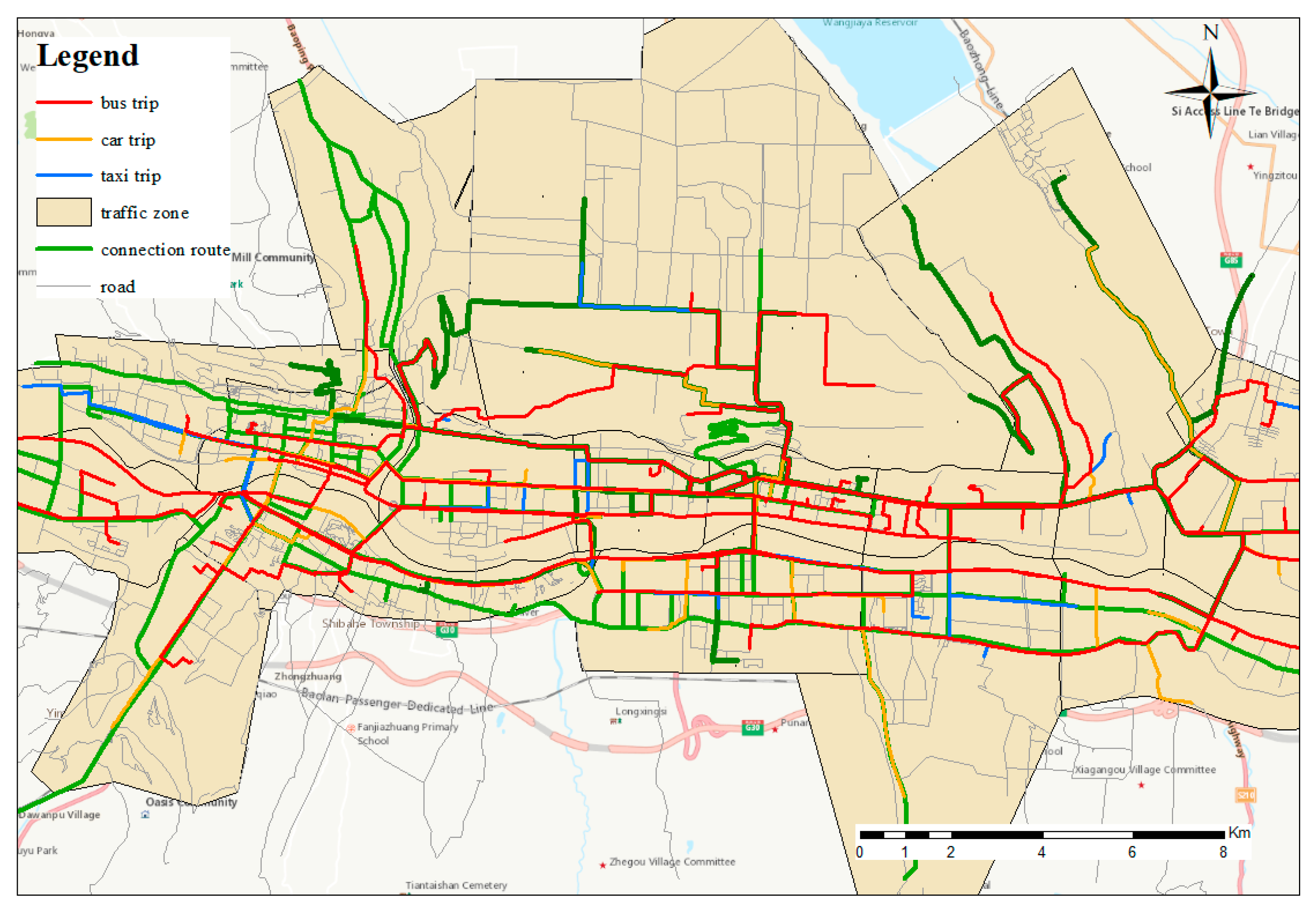
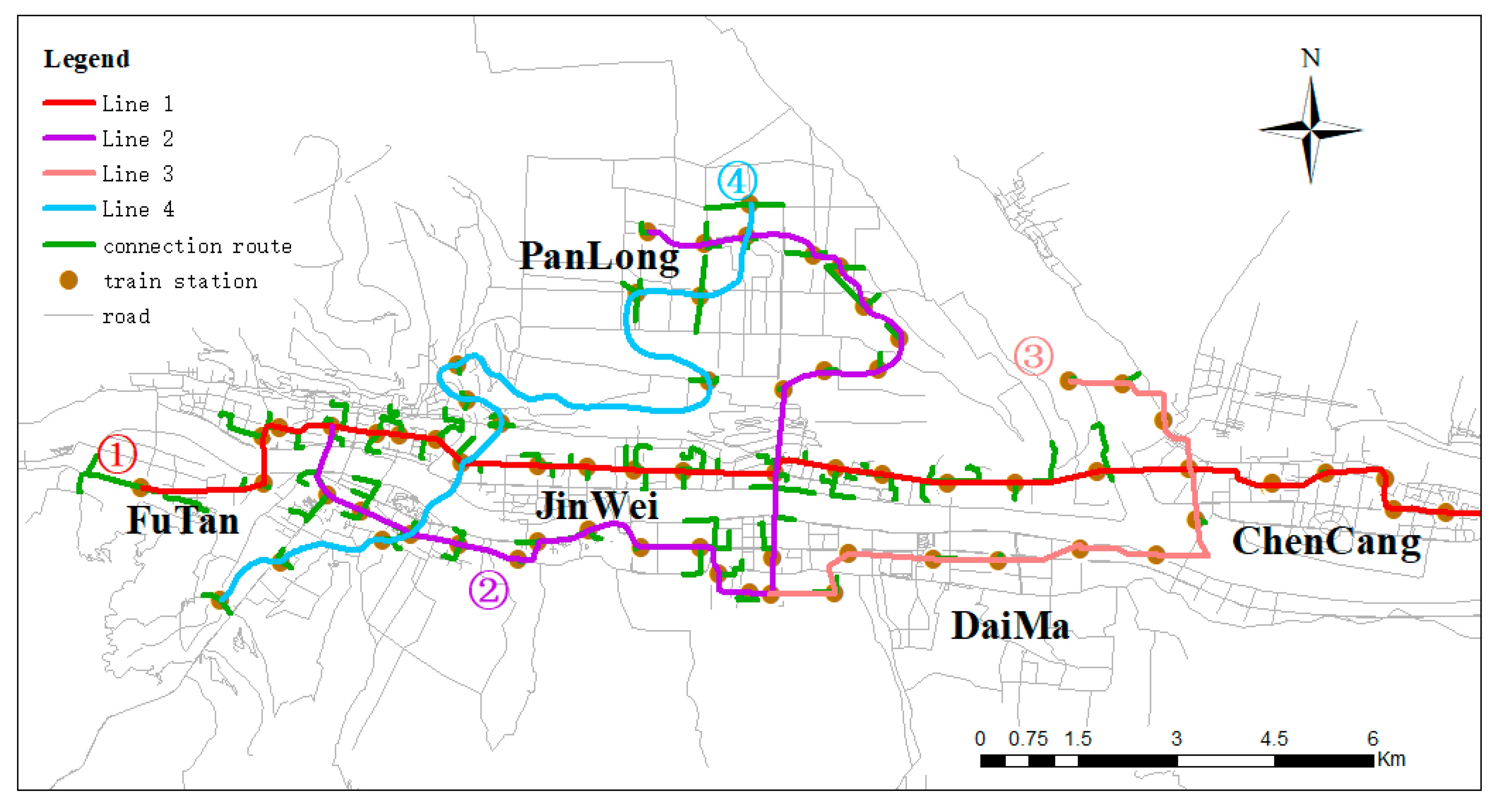
The traditional aggregate model was used in this study to predict passenger demand for the planning year. The travel path was set according to divided traffic zones. The travel distance within one zone and between two zones was calculated. The travel demand for each transportation mode was obtained based on the proportion through Mixed Logit model training. It was assumed that the structure and scale of the city’s road network will not change except for the planned rail transit. Traffic zones 9 and 14 were used as examples to illustrate the extraction method of travel distance. The passenger flow was generated between traffic zones 9 and 14 for the year 2023, while the proportion of rail transit, bus, car, and taxi was predicted. Thus, the travel demands for these four transportations were obtained. This paper provides two reasonable hypotheses to calculate the individual travel distance between two zones. First, the origin and destination for bus travel are set within 500 m of the bus stop; second, the starting point for cars and taxis was established as the centroid position of the traffic zone due to their unfixed stops. The travel OD routes generated on the bus lines, city road network, and rail transit lines are shown in Figure 2 and Figure 3. Through the travel distance combined with the emission factors of buses, cars, taxis, and trail transit, the carbon emissions between traffic zones 9 and 14 were calculated. Similarly, the carbon emissions generated by the demand of passenger trip in other traffic zones could be calculated. The combined calculation of its values shows the carbon emissions of different modes of transportation in Baoji. This provides the necessary parameters for the calculation model of rail transit carbon emission reductions.

3.3. Calculation Model for Urban Rail Carbon Emission Reduction

The cost of carbon or greenhouse gas emission from urban rail transit is related to the lifecycle of its rail infrastructure [36,37,38,39,40]. However, this paper does not address the study of carbon emission caused by the lifecycle assessment of urban rail transit infrastructure, but rather from the perspective of passenger travel demand. By accounting for the size of travel demand attracted by different modes of transportation in cities, two different travel scenarios were constructed to obtain the change of the carbon emissions of urban traffic brought by the transfer of traffic demand between the modes of travel. Based on travel demand for the planning year 2023 [41], we calculated the carbon emissions reduction produced by individual travel activities under two scenarios—With and without rail transit. A model for carbon emission reduction of rail transit is established based on the integrated traffic zone. For Baoji and other cities that do not have open rail transit lines, this paper provides a calculation method of carbon emission reductions brought about by rail transit.

3.3.1. Scenario 1. The scenario without Urban Rail Transit

Under the ‘no urban rail’ scenario in Baoji, 2023, only three transportation modes were considered, including bus, car, and taxi (including online car-hailing). The reasonable travel share rate was obtained by the Mixed Logit model. By taking the divided traffic zone as the unit, the per capita carbon emissions of each mode in every zone was obtained. This, multiplied by the total number of passengers on the target line, gave the sum of the resident trip carbon emissions in traffic zones is calculated. This is considered the baseline value, recorded as C E 0 , which can be calculated using Equation (9):
C E 0 = i = 1 18 k = 1 3 t i · p i k · d i k · E F k + i = 1 18 j i 18 k = 1 3 T i j · P i j k · D i j k · E F k
where C E 0 is the total base carbon emissions produced by passenger travel demand without rail transit;   t i   and   T i j refer to the total number of trips within the ith zone and between the ith and the jth zone, respectively;   p i k   and   P i j k refer to the travel share rate with the kth trip mode within ith zone and from the ith to the jth zone, respectively;   d i k   and   D i j k refer to the travel distance with the kth trip mode within the ith zone and from the ith to the jth zone, respectively;   and   E F k is the carbon emission factor of the kth trip mode.

3.3.2. Scenario 2. The scenario with Urban Rail Transit

The passenger attraction area of rail transit is an uncertain value, but it is best to take walking and cycling into account when considering connection distance. This study defines rail transit connection modes as walking and cycling, so after the opening of urban rail transit in 2023, the total carbon emissions produced by passenger trip demand can be calculated. It is considered that the carbon emissions under this scenario as the current carbon emission value, recorded as C E p , can be calculated using Equation (10):
C E p = i = 1 18 k = 1 3 t i · p i k · d i k · E F k + i = 1 18 j i 18 k = 1 3 T i j · P i j k · D i j k · E F k + m i n j Q m n · D m n · E F l
where C E p is current total carbon emission produced by passenger trip demand with rail transit mode; Q m n is urban rail passengers from the mth station to the nth station; D m n is the urban rail line distance from the mth station to the nth station; m , n is the rail station number of different traffic zones; and   E F l is the carbon emission factor of the lth rail line.
Under the two backgrounds of Scenario 1 and Scenario 2, based on the travel demand of the divided traffic zone, Equations (9) and (10) were used to calculate the urban travel carbon emissions. In scenario 1, urban travel carbon emissions were regarded as the base value,   C E 0 . In scenario 2, urban travel carbon emissions were taken as the current carbon emission value, C E p , so that the travel carbon emission reductions with rail transit can be calculated through Equation (11):
C E r = C E 0 C E p
where C E r is the carbon emission reduction with rail transit as the travel mode.
An important parameter, E F k , is involved in this model. The main modes of transport engaged in this study include bus, car, taxi, and rail transit. The emission factors of different modes should be calculated by the usage amount of different fuel types, fuel net heating value, and fuel burning oxygenation efficiency [42]. Due to the certain difference between China and IPCC based on the emission factors of low heating value, the emission factors in this study uses the emission factors in the Chinese transportation field, and the fuel calorific value is taken from the value in the China Energy Statistical Yearbook 2018. Meanwhile, through fuel consumption, the number of vehicle operations, passenger capacity and vehicle mileage of travel, the collected Baoji transportation energy consumption statistic and the relevant yearbook were used to compare the emission factors database based on vehicle kilometers traveled (VKT) in China. Rail transit mainly uses the city power network for power supply, and the main power consumption uses "Datum Line Emission Factors of Power Grid in Northwest China" for reference. In order to improve the accuracy of carbon emission calculation results, this study selects carbon emission factors in line with the geographical situation of the research object. The relevant fuel value parameters and carbon emission coefficients are shown in Table 2.

4. Results and Discussion

According to current data and the annual economic population growth provided by Baoji Municipal Government, the forecast for total passenger demand of the city in 2023 and the amount of trip OD in the traffic zones were obtained. Meanwhile, based on residents’ travel and individual socio-economic attributes, the Mixed Logit model was used to estimate parameters on the mode of transport choice, and the reasonable distribution of these parameters should obey. Through the training of the property values of resident trips in each zone by the Mixed Logit model, it determined the reasonable parameter distribution and obtained the probability of being selected for each transportation. This study takes this probability as the sharing rate of the travel mode under the condition that the individual travel attributes of the city will not change significantly from the planning year. Subsequently, using the traffic zone divided as a collection unit, the travel path and distance from different transportation demands generated on the road network under rail transit and rail transit free scenarios were determined. This facilitated the calculation of the baseline and current carbon emissions. The difference between these represents the emission reduction that rail transit brings.

4.1. Division of Travel Mode Sharing Rate

The probability of the Mixed Logit model is obtained by the Maximum Simulation Likelihood method. This paper adopts the Mixed Logit Model of Stata software to calibrate the mode choice parameter. The calibration results are shown in Table 3.
In Table 3, the fixed parameters and random parameters are calibrated. The results show that in the commuting and non-commuting models established in this study, the mean of eight random parameters is significant (that is, p < 0.05) and the trend is negative, indicating that an increase in cost and travel time will reduce the utility of each mode to varying degrees. The parameters that are significant in both models include age, income, and car ownership. In the commuting model, rail transit is significant and has a positive impact, indicating that rail transit is more popular than cars. In the non-commuting model, rail transit, taxis, buses, and cars are significant and positive, indicating that the average utility of these four modes has a positive effect on their overall utility. Meanwhile, in terms of socio-economic attributes, age, income, and car ownership are significant in both models, in which income and car ownership are negative and positive, respectively, indicating that high-income car owners are more likely to travel by car. Additionally, the frequency of rail transit is significant in the commuting model, and the positive trend is significant in the non-commuting model as well, indicating that individuals are more inclined to travel by rail. During non-commuting hours, although more choices are available, rail transit still has a high tendency to be used. It can be seen that the introduction of rail transit will have an impact on the daily travel habits of residents. A total of 5500 valid datapoints were used to complete the calibration on the commuting and non-commuting model. After the model converged, the McFadden pseudo-R2 indices were 0.528 and 0.313, both above 0.2, indicating that both models had a good explanatory meaning. Therefore, based on the results of the calibration of each parameter, the travel mode choice probability was predicted, as shown in Table 4, with the parameters subject to the same distribution. The prediction results of non-rail transit mode are shown in brackets.

4.2. Calculation of Rail Transit Carbon Emissions Reduction

According to the calculation formula for the baseline carbon emissions and the travel demands proportion, this paper obtained the OD distance from each mode of transport generated on the road network of the passenger demand in and between the traffic zones, by the GIS network measurement tool. Due to the scale of data generated inside and outside the 18 traffic zones, this study further divided them into five clusters according to administrative area and land utilization. The carbon emissions of these five target clusters were then calculated. Thus, based on the passenger demand, this study obtained the carbon emissions of Baoji in the planning year of 2023 within the context of no rail transit available, as shown in Table 5.
Baseline carbon emissions vary by cluster group. The reason for this is that different groups constitute different traffic zones, so passenger demand and its travel mode and distance generated on the road network significantly differ among clusters. From the perspective of passenger transport mode choice, the total passenger demand determines the amount of carbon emissions. JinWei cluster had the highest passenger demand and its car carbon emissions were the highest, reaching 3.3 t, which is 6.6-times that of buses. Demand for cars is 8% less than that for buses.
The possible reason for this difference is the typical linear city layout of Baoji, where the urban passenger flow corridor extends along an east–west direction, while the development of the north–south line is limited due to the presence of mountains. The JinWei cluster also has a large number of residents traveling through the north–south line, resulting in a significant increase in car travel, thus increasing carbon emissions. Similarly, the demand for buses in the DaiMa cluster is 140,000 higher than that of cars, while the carbon emissions of cars remained the largest, followed by taxi (including online car-hailing) at 6.6 and 4.3 times the carbon footprint of buses, respectively. In the situation of benchmark carbon emission calculation, the proportion of public transport travel is about 44%. The insufficient bus lines, the large east–west distance span, and high station demand for a route with limited capacity, leaves the public transportation system struggling. In the absence of rail transit, passengers will choose buses, cars, and taxis to travel, prolonging the average travel distance and resulting in higher carbon emissions.
Based on the approved plan for the urban rail transit network in Baoji, the annual operating energy consumption of the subway system and the baseline carbon emission coefficient of the North China Power Grid, as well as the current carbon emission calculation model, the carbon emissions based on passenger demand after the opening of the rail transit line in 2023 were calculated. The results are shown in Table 6.
There are four rail lines planned to be built in the planning year of 2023. Line 1 runs through FuTan and ChenCang clusters at both ends of Baoji from east to west. Its length will reach 40.9 km with 33 stations, which will significantly alleviate pressure on bus lines. After its opening, bus passenger demand in FuTan cluster and ChenCang cluster is predicted to decrease by 6% and 7%, respectively. Rail and public transport are mostly flat in carbon emissions, much lower than for cars and taxis. At the same time, rail lines 1, 2, and 4 all pass through JinWei cluster, making the current carbon emissions 41% of the baseline carbon emissions, becoming the most significant carbon emission reducing area. JinWei cluster, which has the highest passenger demand, accounts for up to 50% of passenger traffic in the city’s public transport system, which includes not only passengers from bus to rail transit but also those induced by the stations along the rail transit route. The PanLong and DaiMa clusters are located on the north and south sides of the central part of Baoji. The transportation network density is low there due to the small size of the north–south network. Lines 2 and 4 have alleviated the transportation pressure of the north–south transport corridors, moving passenger traffic to rail transit from cars and taxis, reducing their carbon footprint to 60 t. In the PanLong and DaiMa clusters, due to their special geographic positions in the northern and southern areas of central Baoji, the south–north traffic network there has a small scale and the public transport network has a low density. The establishment of Line 2 and Line 4 has reduced the pressure on the north–south corridor of urban traffic, so that the passengers of cars and taxis have been transferred to the rail transit; thus, the carbon emissions of cars and taxis will be significantly reduced to 60 tons of CO2.
This study calculated the baseline and current carbon emissions of traffic clusters under the two scenarios of Baoji for the planning year 2023. Traffic clusters based on the urban passenger demand reflect land use, geographical location, and individual travel OD. After the opening of the urban rail lines in Baoji, these five clusters will have an annual emission reduction of 1070 tons of CO2. The results are shown in Table 7. The total emission reduction for each cluster is directly related to its annual demand. Urban rail transit has become an important means of transportation, with four lines designed to meet passenger demand across five traffic clusters. Regardless of the degree of satisfaction for passenger demand, the current carbon emission of each cluster is much smaller than the baseline emission. The highest carbon reduction is expected to be in the FuTan cluster, where there are three transit stations for lines 1, 2, and 4. Individuals can use rail transit to complete their trip. Thus, its reduction in carbon emissions per capita is the highest. The lowest reduction is expected to be for the residents in PanLong cluster, due to its low demand and the existence of the PanLong bus hub station, which will attract some of the passengers [43]. In short, after the completion of the Baoji rail transit by 2023, accompanied by higher passenger demand, carbon emissions will drop significantly [44]. Therefore, the strategic decision of Baoji to open urban rail transit in the planning year has a certain theoretical basis and practical significance.

5. Conclusions

The carbon emission reduction model based on passenger demand is the basis of the transportation planning four-stage model. This paper calculated the passengers’ OD travel route and distance for each mode of transport within the road network on the level of urban passenger trip demand. It then calculated the carbon emission reduction of the planning year 2023 in Baoji with or without rail transit. There were two assumptions made in the model construction of this paper: We assumed that the travel attributes of urban residents and their socio-economic attributes will not change significantly by 2023; and we assumed that the road network of Baoji does not change significantly from the planning year, while the bus routes and stops will remain as they are in the current situation. The data used in this study are from the year 2018, compared with the planning year 2023; this short time span makes the limitations of these two necessary assumptions negligible. Therefore, this paper used the survey data to establish a model to discover the determinants of residents’ travel choices. Furthermore, we forecasted the probability of different transportation modes being chosen using valid trip attribute data. For cities that do not have urban rail transit lines, according to the line designs approved and the OD demand of passengers within traffic zones, this paper calculated the carbon emission model under two scenarios, that is, with or without rail transit. The following conclusions have been drawn based on emission models and results.
(1). The demand for commuting passenger flows is more sensitive to travel by urban rail transit, and the probability of choosing this utility branch value is high.
(2). If urban rail transit is not available in 2023, the transportation carbon emissions of Baoji will reach 20,400 tons of carbon dioxide, with an increase of passenger travel demand, of which 57.6% will come from cars. At this time, restricting automobile journeys will be the primary measure for reducing carbon emissions.
(3). The current public transport pressure in Baoji is high, and its proportion of transport mode share accounts for 42.4%. At the same time, the per capita carbon emissions of public transport are relatively high, accounting for 52.7% of the total emissions of residents. This highlights the need for sustained and stable development of public transport.
(4). If urban rail transit runs in 2023, the proportion of passenger vehicles for Baoji will decrease by 16.2%, and that of public transportation will increase by 23.4%. Rail transit will significantly alleviate traffic pressure on the east–west corridor (with the topographic watercourse feature) in Baoji and achieve a carbon reduction of 1070 tons of carbon dioxide.
(5). Taking into account the energy and power carbon emissions of rail transit stations, the emissions per person of rail transit are at least about 32 g CO2 per kilometer higher than that of buses. However, urban rail transit has a large-capacity, timely and efficient operational capability, which cannot be replaced by other means of transport. Therefore, the opening of the urban rail transit has important practical significance for Baoji.
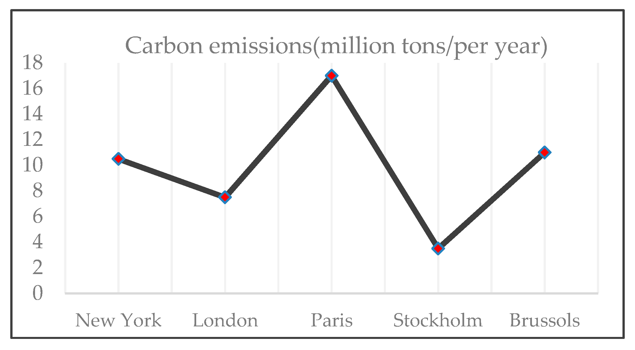
Comparison of Baoji’s emissions with that of other cities in the world is helpful for emission mitigation policymaking. Firstly, latest researches on carbon emissions of urban transportation of cities in Continental Europe [45], the UK [46], and America [47] were collected, shown in Figure 4. However, most of the released emission inventories do not provide the details of the estimation, such as transport modes covered. Therefore, it is challenging to split emissions precisely according to the scope of this work. However, a general comparison without considering background information still can tell us something about the current emissions of developed countries, such as those cities have long been well aware of the problem and are seeking ways to reduce emissions, and some laws have been introduced to reduce GHG mitigation. Baoji has the potential to reduce emissions learning from experience. Secondly, researches have been carried out in China. Peng Binbin [48] established an urban passenger transport energy saving and emission reduction potential evaluation model. This was used to evaluate the reduction potential of final energy consumption, GHG emissions and pollutants emissions of Tianjin’s urban passenger transport sector between 2010 and 2040. The evaluation was conducted under four scenarios, namely Business as Usual (BAU) scenario, the 12th five-year Plan Policy (PP) scenario, Comprehensive Policy (CP) scenario, and hybrid policy of PP and CP (HP) scenario. This method calculates and compares the carbon emission of passenger transport under different scenarios, obtains the energy-saving and emission reduction potential of urban passenger transport, which is reasonable and effective. Chen Feng introduced a carbon reduction method for rail transit. A measurement model that takes the passenger carbon emissions before the line is opened as the baseline and compares these with the standard after the opening, thus determining the carbon emissions reduction [18]. This model was applied to rail transit lines that have been opened in Beijing in recent years. The emissions reductions of four different routes were estimated, and the carbon emission reduction effect of rail transit was evaluated. These models mentioned are similar to the methods in this paper. They all calculate the carbon emissions under different scenarios to determine the potential emission reduction of urban passenger transport. Furthermore, the cases study of the different cities proves that these methods are reasonable and have reference value for further researches.
In China, a city with a medium-sized population and economy such as Baoji has a good development trend and is a growing city. The rapid increase in passenger demand manifests the rapid development of such cities. However, there are few studies that have calculated the extent to which the opening of urban rail transit will reduce carbon emissions from transportation. Therefore, when planning the rail transit network, such cities can use survey data and the line designs, through the calculation method of this paper, to quantitatively determine the carbon emissions reduction. This method provides quantitative theoretical support for the construction of low-carbon and environmentally friendly rail transit in such cities.

Author Contributions

Z.W. and F.C. conceived and designed the research framework. N.Z. established the model; Z.W. and Y.L. calibrated performed the survey; J.S. and J.W. calibrated performed the survey; J.W. and Y.L. analyzed the data and calculated the carbon reduction; N.Z. and Z.W. wrote the paper. All authors have read and agreed to the published version of the manuscript.

Funding

The work described herein is part of a research project on ‘‘Investigation Report on Comprehensive Traffic and Resident Travel in Baoji City in 2017’’ funded by from China Railway Engineering Design Consulting Group Co., LTD, China and has been funded by the National Natural Science Foundation of China (No.7187027). The authors thank the reviewers for their helpful comments.

Conflicts of Interest

The authors declare no conflict of interest.

References

  1. Jiang, H.; Bai, F. Research on low carbon economy evaluation of Urban Rail Transit. Railw. Transp. Econ. 2010, 32, 11–15. [Google Scholar]
  2. Li, X.; Yu, B.Y. Peaking CO2 Emissions for China’s Urban Passenger Transport Sector. Energy Policy 2019, 10, 1–18. [Google Scholar] [CrossRef]
  3. Pucher, J.; Peng, Z.R.; Mittal, N.; Zhu, Y.; Korattyswaroopam, N. Urban Transport Trends and Policies in China and India: Impacts of Rapid Economic Growth. Transp. Rev. 2007, 27, 379–410. [Google Scholar] [CrossRef]
  4. Bao, X.D. Urban Rail Transit Present Situation and Future Development Trends in China: Overall Analysis Based on National Policies and Strategic Plans in 2016–2020. Urban Rail Transit 2018, 4, 1–12. [Google Scholar] [CrossRef] [Green Version]
  5. Lu, K.; Han, B.M.; Lu, F.; Wang, Z.J. Urban Rail Transit in China: Progress Report and Analysis (2008–2015). Urban Rail Transit 2016, 2, 93–105. [Google Scholar] [CrossRef] [Green Version]
  6. Yuan, R.Q.; Tao, X.; Yang, X.L. CO2 Emission of Urban Passenger Transportation in China from 2000 to 2014. Adv. Clim. Chang. Res. 2019, 10, 59–67. [Google Scholar] [CrossRef]
  7. Wang, H.H.; Zeng, W.H. Revealing Urban Carbon Dioxide (CO2 ) Emission Characteristics and Influencing Mechanisms from the Perspective of Commuting. Sustainability 2019, 11, 385. [Google Scholar] [CrossRef] [Green Version]
  8. Ecola, L.; Zmud, J.; Gu, K.; Phleps, P.; Feige, I. The Future of Mobility: Scenarios for China in 2030. RAND Institute for Mobility Research; Deloite University Press: Santa Monica, CA, USA, 2015. [Google Scholar]
  9. Xu, W.; Guthrie, A.; Fan, Y.; Li, Y. Transit-Oriented Development: Literature Review and Evaluation of TOD Potential across 50 Chinese Cities. J. Transp. Land Use 2017, 10, 743–762. [Google Scholar] [CrossRef] [Green Version]
  10. Li, G.Q.; Li, Q.Q.; Zhuang, Y.; Yue, Y.; Liu, Z.Z.; Li, S.Q.; Daniel, S. Urban Commuting Dynamics in Response to Public Transit Upgrades: A Big Data Approach. PLoS ONE 2019, 14, e0223650. [Google Scholar]
  11. Wu, W.J.; Liang, Y.T.; Wu, D. Evaluating the Impact of China’s Rail Network Expansions on Local Accessibility: A Market Potential Approach. Sustainability 2016, 8, 512. [Google Scholar] [CrossRef] [Green Version]
  12. Boarnet Marlon, G.; Wang, X.Z.; Douglas, H. Can New Light Rail Reduce Personal Vehicle Carbon Emissions? A Before-After, Experimental-Control Evaluation in Los Angeles. J. Reg. Sci. 2017, 57, 523–539. [Google Scholar] [CrossRef] [Green Version]
  13. Kwan, S.C.; Tainio, M.; Woodcock, J.; Sutan, R.; Hashim, J.H. The Carbon Savings and Health Co-Benefits from the Introduction of Mass Rapid Transit System in Greater Kuala Lumpur, Malaysia. J. Transp. Health 2017, 6, 187–200. [Google Scholar] [CrossRef]
  14. Wu, S.M.; Pei, Y.L.; Cheng, G.Z. The study of urban traffic modal splitting method based on MD model under the low-carbon mode. Comput. Model. New Technol. 2014, 18, 197–202. [Google Scholar]
  15. Wang, Z.J.; Chen, F.; Fujiyama, T. Carbon emission from urban passenger transportation in Beijing. Transp. Res. Part D Transp. Environ. 2015, 41, 217–227. [Google Scholar] [CrossRef]
  16. Li, L.; Hu, J.; Shao, D. The carbon emission reduction benefits of the rapid development of Shanghai Expo. China Environ. Sci. 2012, 32, 1141–1147. [Google Scholar]
  17. Board, C.E. Approved Consolidated Baseline and Monitoring Methodology ACM0016—Baseline Methodology for Mass Rapid Transit Projects; UNFCCC: Rio de Janeiro, Brazil; CCNUCC: Rio de Janeiro, Brazil, 2011. [Google Scholar]
  18. Chen, F.; Shen, X.P.; Wang, Z.J.; Yang, Y. An Evaluation of the Low-Carbon Effects of Urban Rail Based On Mode Shifts. Sustainability 2017, 9, 401. [Google Scholar] [CrossRef] [Green Version]
  19. Hiroshi, O. Planning of urban rail transit system in Tokyo, Construction and management. Res. Urban Rail Transit 2003, 3, 1–7. (In Japanese) [Google Scholar]
  20. Li, Z.; Li, C.; Liao, K. Research and Practice of Monitoring and Evaluation on Carbon Emission from Urban Transport; China Communications Press Co., Ltd: Beijing, China, 2017; ISBN 978-7-114-14073-0.201. [Google Scholar]
  21. Baoji Municipal Commission of Urban and Rural Planning. In Baoji’s Urban Rail Transit Network Construction Plan (2017–2023); Baoji Municipal Government: Baoji, China, 2016.
  22. Chang’an University. Survey on Comprehensive Transportation and Urban Residents’ Travel in Baoji, 2014 and Supplementary Traffic Survey in 2017; Baoji Municipal People’s Government: Baoji, China, 2017.
  23. Baoji Transportation Bureau. Baoji Traffic Development Annual Report, 2009–2018; Baoji, China, 2018.
  24. Baoji Municipal People’s Government Office. Assessment of Energy Saving, Carbon Emission Reduction and Coal Reduction in 2017; Baoji, China, 2017.
  25. Lin, J.W.; Shen, P.; Lee, B.J. Repetitive model refinement for questionnaire design improvement in the evaluation of working characteristics in construction enterprises. Sustainability 2015, 7, 15179–15193. [Google Scholar] [CrossRef] [Green Version]
  26. National Development and Reform Commission of China. 2017 Baseline Emission Factors for Regional Power Grids in China; China Statistics Press: Beijing, China, 2017. (In Chinese) [Google Scholar]
  27. National Bureau of Statistics of China. China Energy Statistical Yearbook 2018; China Statistics Press: Beijing, China, 2019.
  28. Wang, Z.J.; Chen, F.; Shi, Z. Prediction on medium and long term energy consumption of urban rail transit network in Beijing. China Railw. Sci. 2013, 4, 133–136. [Google Scholar]
  29. Ma, C.; Wang, Y.; Guo, Y. Sensitivity analysis on urban rail transit passenger flow forecast. In Proceedings of the 2011 International Conference on Electric Technology & Civil Engineering, Lushan, China, 22–24 April 2011. [Google Scholar]
  30. Wang, S.S.; Huang, W.; Lu, Z.B. Study on Mixed Logit Model and Its Application in Traffic Mode Split. J. Highw. Transp. Res. Dev. 2006, 5, 88–91. (In Chinese) [Google Scholar]
  31. McFadden, D.; Train, K. Mixed MNL models for discrete response. J. Appl. Econom. 2000, 15, 447–470. [Google Scholar] [CrossRef]
  32. Li, H.; Huang, H.; Liu, J. Parameter Estimation of the Mixed Logit model and Its Application. J. Transp. Systems Eng. Inf. Technol. 2010, 10, 73–78. [Google Scholar] [CrossRef]
  33. Wen, C.H.; Koppelman, F.S. The generalized nested logit model. Transp. Res. B 2001, 35, 627–641. [Google Scholar] [CrossRef] [Green Version]
  34. He, M.; Guo, X.C.; Ran, J.Y. Forecasting Rail Transit Split with Disaggregated MNL Model. J. Transp. Syst. Eng. Inf. Technol. 2010, 10, 136–142. [Google Scholar] [CrossRef]
  35. Song, X.M.; Jiang, Y.S.; Yun, L. Study on the calculation method of MD forecast model. J. Transp. Eng. Inf. 2010, 2, 65–70. [Google Scholar]
  36. Baron, T.; Tuchschmid, M.; Martinetti, G.; Pépion, D. High Speed Rail and Sustainability. In Background Report: Methodology and Results of Carbon Footprint Analysis; International Union of Railways (UIC): Paris, France, 2011. [Google Scholar]
  37. Cuenot, F.; Gabriel, C.H. Carbon Footprint of Railway Infrastructure. Comparing Existing Methodologies on Typical Corridors. Recommendations for Harmonized Approach. 2016. Available online: https://uic.org/IMG/pdf/carbon_footprint_of_railway_infrastructure.pdf (accessed on 12 July 2016).
  38. Network Rail. Comparing the Environmental Impact of Conventional and High Speed Rail; Milton Keynes, Bucks: London, Britain, 2009. [Google Scholar]
  39. Olugbenga, O.; Kalyviotis, N.; Saxe, S. Embodied Emissions in Rail Infrastructure: A Critical Literature Review. Environ. Res. Lett. 2019, 14, 123002. [Google Scholar] [CrossRef] [Green Version]
  40. Egis. Introduction to Greenhouse Gas Emissions in Road Construction and Rehabilitation. 2010. Available online: https://www.google.co.th/url?sa=t&rct=j&q=&esrc=s&source=web&cd=3&cad=rja&uact=8&ved=0ahUKEwi4uu_k9tXKAhWFHY4KHZENDoMQFggtMAI&url=http://siteresources.worldbank.org/INTEAPASTAE/Resources/GHG-ExecSummary.pdf&usg=AFQjCNESVUT_Mx6NmMOUjLHSUo6QXCMo (accessed on 1 November 2010).
  41. Chang’an University. Research of the Passenger Flow Demand Forecast on Urban Rail Transit Network Planning of Baoji; China Railway Engineering Consultants Group Co., LTD: Beijing, China, May 2017. (In Chinese) [Google Scholar]
  42. General Administration of Quality Supervision, Inspection and Quarantine of China. Test Methods for Fuel Consumption of CNG Vehicles; GB/T 29125-2012; China Standards Press: Beijing, China, 2012. (In Chinese) [Google Scholar]
  43. Xia, H.; Li, X. Study on Intensive Design of Urban Rail Transport Hub from the Perspective of Low-Carbon; Springer: Berlin/Heidelberg, Germany, 2012; pp. 409–415. [Google Scholar]
  44. Baoji Urban Rail Transit Construction Co., Ltd. Study on the environmental impact of Baoji’s Urban Rail Transit Construction Plan (2017–2023); Baoji Urban Rail Transit Construction Co., Ltd. Baoji Municipal Government: Baoji, China, 2017. [Google Scholar]
  45. Carney, S.; Green, N.; Wood, R.; Read, R. Greenhouse Gas Emissions Inventories for 18 European Regions. 2009. Available online: http://www.euco2.eu/resources/GRIPBroschuere-Small.pdf (accessed on 30 November 2015).
  46. Ricardo-AEA. Local and Regional CO2 Emissions Estimates for 2005–2011—CO2 Emissions Within the Scope of Influence of Local Authorities (Previously Called National Indicator 186: Per Capita CO2 Emissions in the LA Area), Department of Energy and Climate Change, London. 2013. Available online: https://www.gov.uk/government/uploads/system/uploads/attachment_data/file/212448/Copy_of_Subset_Datatables.xlsx (accessed on 22 January 2013).
  47. Dickinson, J.; Khan, J.; Amar, M. Inventory of New York City Greenhouse Gas Emissions; City of New York, Mayor’s Office of Long-Term Planning and Sustainability: New York, NY, USA, 2013; Available online: http://nytelecom.vo.llnwd.net/o15/agencies/planyc2030/pdf/greenhousegas_2013.pdf (accessed on 1 April 2007).
  48. Peng, B.B.; Du, H.B.; Ma, S.F.; Fan, Y.; David, C. Broadstock. Urban passenger transport energy saving and emission reduction potential: A case study for Tianjin, China. Energy Convers. Manag. 2015, 102, 4–16. [Google Scholar] [CrossRef]
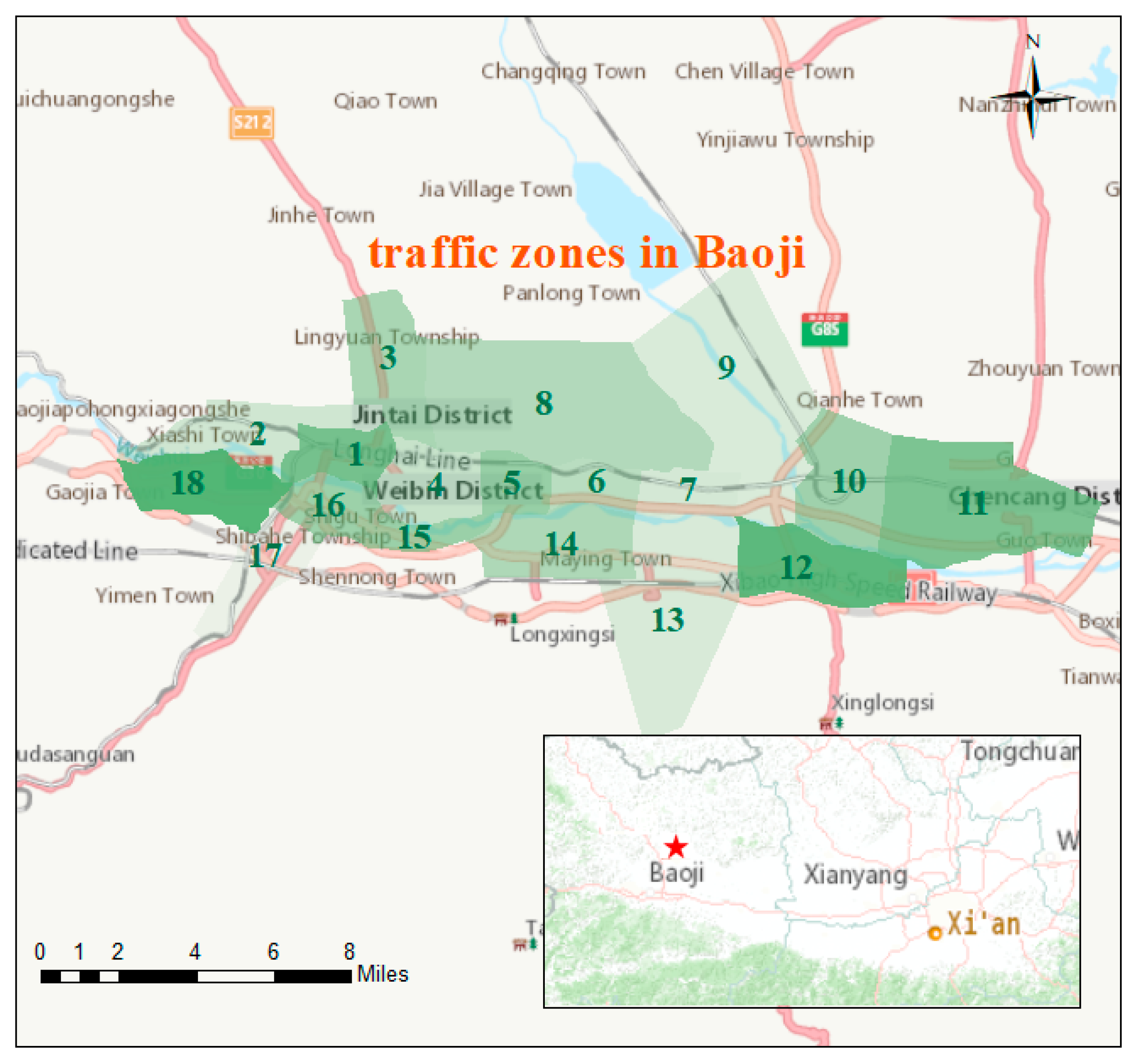
Figure 1. Division of Baoji traffic zones.
Energies 13 00782 g001
Figure 2. Origin-destination (OD) routes for individual by bus, car, and taxi.
Energies 13 00782 g002
Figure 3. OD routes for individuals on road network of rail transit.
Energies 13 00782 g003
Figure 4. Carbon emissions from passenger transportation of different cities.
Energies 13 00782 g004
Table 1. Attribute level and coding.
ParameterTypeCode
Trip attribute (X)trip purpose Xpucommute trip:1; not commute trip:-1;
trip original time Xstcommute trip: flat hour: −1; peak hour (7:00–8:00 and 18:30–19:30): 1; not commute: flat hour: −1; peak hour (19:00 and 22:00): 1;
trip distance Xtd (km)(0,5]: −1; (5,10]: 0; (10,15]: 1;
arrival time Xat (min)bus: [10,60]; car: [5,40]; taxi: [15,30]; rail: [10,30]; values from −1; 0; 1; −1 represents low; 0 represents middle; and 1 represents high
mode speed Xmv (km/h)bus: [20,40]; car:[40,80]; taxi: [50,60]; rail: [40,60]; value from −1; 0; 1; −1 represent low; 0 represents middle; and 1 represents high
trip fare Xf (RMB/km)bus: 1; 2; 4; car: 1.2; 1.5; 1.8; taxi:1.5; 2.4; 3.5; rail:4; 6; 8;
value from −1; 0; 1; −1 represent low; 0 represents middle; and 1 represents high
Socioeconomic attribute (O)gendermale: 1; female: 2
age[6,20): −2; [20,40): −1; [40,60): 1; [60,80): 2
occupationpersonnel of enterprises or institutions: −2; individual, student, other: −1; retirees, farmers, unemployed persons: 1
income (RMB)<3000: −2; (3000,5000]: −1; (5000,7500]: 1; >7500: 2
Frequency of urban rail used (times/day)>2:1; 1–2:1; none: 0
trip origin-destination (OD) from traffic zonesoriginal zone and destination zone from zone [1,18]
Table 2. Carbon emission factor for fuel and modes.
Fuel TypeConverted Standard Coal Coefficient (t/105 Kmh)Converted Benchmark Oil Coefficient (t/105 Kmh)Density (p/m3)Emission Factor (t/105 m3)
Gasoline13.39.31-21.84
CNG1.47141.030.742.9849
Diesel1.45711.020.863.1605
Northwest China GridCarbon emission (million t CO2)Generation capacity (108 KWh)Grid carbon emission factor (kg/KWh)Sharing of power supply (%)
321.3446110.69692.67
ModesRail transitBusesTaxisCars
Emission factor (g CO2/PKM)4942.1191.1146.9
Table 3. Choice of model calibration results based on the Mixed Logit Model.
AttributeParameterCommuting ModeNon-Commuting Mode
Random Valuesp ValueRandom Valuesp Value
Gender β g e n 0.2050.4820.1820.356
Age β a g e 0.214 ***0.0130.194 **0.018
Occupation β o c c 0.3770.0760.2240.046
Income β i n c −0.371 ***0.001−0.213 ***0.000
Car ownership β c a r 1.061 **0.0002.156 ***0.000
Trip purpose β p u 0.0720.027−0.147 **0.053
Departure time β s t 0.2170.371−0.1080.322
Arrival time β a t −2.7750.000−3.144 *0.001
Trip distance β t d 0.219 **0.025−0.1360.057
Fare β f b u s −4.035 ***0.000−0.375 **0.001
β f c a r −7.653 ***0.003−1.642 ***0.000
β f t a x −2.031 ***0.002−3.672 ***0.001
β f r a i −1.721 ***0.018−2.786 **0.014
Travel time β t b u s −2.75 **0.000−3.623 ***0.000
β t c a r −2.221 ***0.014−3.015 ***0.000
β t t a x −2.672 ***0.000−3.135 ***0.000
β t r a i −3.015 ***0.000−2.941 **0.001
Bus intrinsic constant A S C b u s −0.3150.6770.4110.301
Car intrinsic constant A S C c a r –0.901 *0.0852.715 ***0.000
Taxi intrinsic A S C t a x −1.0120.0221.354 **0.011
Rail transit intrinsic A S C r a i 0.914 ***0.0231.1280.001
Rail trip frequency β f 0.474 **0.0050.174 *0.892
Effective samples55005500
McFadden Pseudo R20.5280.313
Notes: *p < 0.1, **p < 0.01, ***p < 0.05.
Table 4. Proportion of journeys made using each mode of transport.
ModesBusesRail TransitCarsTaxi (Taxi-Hailing)
ratio0.34 (0.42)0.31 (0.0)0.19 (0.35)0.16 (0.23)
Table 5. Annual carbon emissions under the baseline scenario in Baoji, 2023, showing traffic cluster groups.
Cluster NameConstituted Traffic ZoneAnnual Demand (Thousand Persons)Average Travel Distance of Road Network(km)Carbon Emissions by Transport Mode(t CO2)Base Carbon Emissions (t CO2)
BusCarTaxiBusCarTaxiBusCarTaxi
FuTan2,1840%36%24%22.877.546.30.22.21.13.5
JinWei1,4,15,16,1741%33%26%21.952.941.10.53.32.76.5
PanLong845%32%23%14.844.634.20.11.00.71.9
DaiMa5,6,7,13,1447%30%23%19.954.137.00.32.01.33.6
ChenCang9,10,1141%34%25%31.564.851.20.42.61.94.9
Table 6. Annual carbon emissions for the urban rail scenario in Baoji, 2023 based on traffic cluster groups.
Cluster NameAnnual Demand (Thousand Persons)Modes Carbon Emissions (Hundred T CO2)Total Annual Direct Carbon Emissions (Hundred T CO2)
BusRail TransitCarTaxiBusRail TransitCarTaxi
FuTan34%29%19%18%0.20.20.70.51.6
JinWei33%32%18%17%0.20.21.21.12.7
PanLong34%27%20%19%0.10.10.50.31.1
DaiMa34%29%18%19%0.20.20.60.71.7
ChenCang34%30%19%17%0.30.31.30.82.6
Table 7. Total emission reduction of traffic travel demand in Baoji, 2023 based on traffic cluster groups.
Cluster NameAnnual Passenger VolumeAnnual Emissions ReductionCarbon Emissions Reduction Per Passenger
Thousand PersonsHundred T CO2 g CO2/Person
FuTan525.41.9358.9
JinWei1300.53.7287.1
PanLong487.90.8167.0
DaiMa827.11.9234.9
ChenCang787.22.3292.6