Abstract
Traditional acoustic evaluation of a diesel engine generally uses the A-weighted sound pressure level (AWSPL) and radiated sound power to assess the noise of an engine prototype present in an experiment. However, this cannot accurately and comprehensively reflect the auditory senses of human subjects during the simulation stage. To overcome such shortage, the Moore–Glasberg loudness and sharpness approach is applied to evaluate and improve the sound quality (SQ) of a 16 V-type marine diesel engine, and synthesizing noise audio files. Through finite element (FE) simulations, the modes of the engine’s block and the average vibrational velocity of the entire engine surface were calculated and compared with the test results. By further applying an automatically matched layer (AML) approach, the engine-radiated sound pressure level (SPL) and sound power contributions of all engine parts were obtained. By analyzing the Moore–Glasberg loudness and sharpness characteristics of three critical sound field points, an improvement strategy of the oil sump was then proposed. After improvement, both the loudness and sharpness decreased significantly. To verify the objective SQ evaluation results, ten noise audio clips of the diesel engine were then synthesized and tested. The subjective evaluation results were in accordance with the simulated analysis. Therefore, the proposed approach to analyze and improve the SQ of a diesel engine is reliable and effective.
1. Introduction
Due to the high-speed and power development trend of marine diesel engines, their vibration and noise issues are becoming more significant. Thus, the noise, vibration, and harshness (NVH) performance of them urgently needs improvement. Using the traditional A-weighted sound pressure level (AWSPL) and radiated sound power metrics sometimes leads to a phenomenon in which the evaluation results of some noise may be acceptable but is still disturbing to human subjects. Therefore, the sound quality (SQ), which is used to study the human listening procedure in detail, has rapidly developed. However, most previous SQ studies on diesel engines have been based on the test data, which is unable to predict the noise problems comprehensively. The aim of this study is therefore to evaluate and improve the SQ of a 16 V-type marine diesel engine based on the simulation and test to verify the improvement effects.
Both loudness and sharpness are important objective evaluation parameters to investigate the SQ. Zwicker and Moore–Glasberg are two main loudness models. The total Zwicker loudness has been applied to not only the radiated noise of internal combustion engines [1,2,3], but also the interior noise of gasoline vehicles [4,5,6], electric vehicles, and high-speed trains [7,8].
However, just a few studies have focused on the distribution and variation of the specific loudness. Ishibashi et al. [9] compared the sound pressure level (SPL) with the Zwicker specific loudness of 70 types of environmental noise within the frequency range of 63–4000 Hz, pointing out that they have a strong correlation. Yoon et al. [10] compared the Zwicker specific loudness of passing noise between freight trains and subways and determined that noises within frequencies of 20–300 and 2700–4400 Hz have a greater influence on the human perception. Luo et al. [11] compared the Moore–Glasberg specific loudness with the SPL spectrum, applying them on both colored noise and high-speed train interior noise, proving that the loudness metric can reflect the characteristics of sound and human sensations. Yan and Jiang [12] combined the Zwicker specific loudness with an operational path analysis to assess the SQ contributions that a commercial micro-car’s panels made toward its interior noise. Valverde et al. [13] used the Zwicker specific loudness to evaluate the noise of 18 automotive mechanical push-buttons and concluded that high-frequency components have the greatest contribution.
The above studies of specific loudness are all based on noise signals obtained from experiments. If the specific loudness can be predicted and improved during the simulation stage, the research efficiency will increase, and the costs will decrease. Kook et al. [14] improved the structural distribution of the reflective materials used in noise barriers through a simulation method. The sound insulation performance showed that using the Zwicker specific loudness to guide the optimization of the noise barriers is more reliable than a 1/3 octave SPL. Mao et al. [15] improved the Zwicker loudness of a four-cylinder diesel engine using the multi-body dynamics method. Later, Mao et al. [16] replaced the critical band with the equivalent rectangular bandwidth (ERB). However, they did not analyze the Moore–Glasberg specific loudness distribution characteristics in detail. Fan et al. [17] identified the acoustic contribution of panels of an elastic cavity using the Moore–Glasberg specific loudness, which was proven to be effective, although they only focused on the low-frequency noise.
When calculating the excitation level, the Moore–Glasberg model divides the human auditory frequency range (20–20,000 Hz) into 372 sub-bands which are from 1.8 to 38.9 Cams with an interval of 0.1 Cam [18]. That is more than Zwicker’s 24 sub-bands [19] which are from 1 to 24 Bark with an interval of 1 Bark. The central frequency of each ERB band, and the low- and high-boundary frequencies of each critical band are depicted in Figure 1.
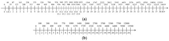
Figure 1.
Frequency distribution characteristics of equivalent rectangular bandwidth ERB and critical bands. (a) Central frequencies of ERB bands; (b) Boundary frequencies of critical bands.
Figure 2 shows the bandwidths of ERB and critical bands as a function of frequency. The bandwidth of the ERB band is about 25 Hz in the low frequency range and leveling up to about 11% of the center frequency at high frequencies [20], generally narrower than the critical band.
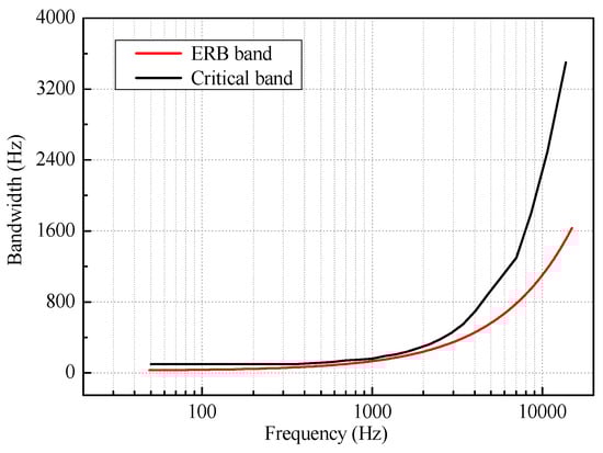
Figure 2.
Bandwidths of ERB and critical bands.
Because the major frequency range of the diesel engine noise was much narrower than 20,000 Hz, it needs to be divided more finely to find the problematic frequency band in detail. Additionally, accounting for the operating conditions of the diesel engine applied were under a steady state, the Moore–Glasberg loudness model, standardized as ANSI S3.4:2007 [21], was chosen in this study.
The sharpness calculation is based on the specific loudness [19]. To date, only the sharpness generated from the Zwicker specific loudness has been standardized (as DIN 45692:2009 [22]) and applied in numerous SQ studies [23,24,25,26,27,28,29]. To calculate the sharpness using the Moore–Glasberg specific loudness, the method proposed by Swift and Gee [30,31] was applied in this study.
In the development process of the diesel engine, with the continuous improvement of the vibrational and acoustic standards, traditional evaluation indicators such as AWSPL and the radiated sound power are no longer able to accurately assess the subjective auditory sensations of human subjects toward diesel engine noise. In contrast, most SQ objective and subjective evaluations of diesel engine noise have been based on signals acquired from acoustic tests of a prototype, which cannot be realized in the simulation stage of the research and development. Under this premise, a 16 V-type marine diesel engine was studied by combining finite element (FE) and automatically matched layer (AML) analyses to investigate its natural modes, dynamic responses, and radiated noise characteristics. The noise characteristics were then analyzed by calculating the sound power contribution of five engine parts, and the Moore–Glasberg specific loudness and sharpness of three sound field points. The structure, acoustics, and SQ analysis results indicate that the oil sump is the key noise radiation part, therefore the strengthening ribs are utilized to improve the SQ of oil sump. Based on such improvement, SQ analyses were further conducted. Their noise audio clips were synthesized using MATLAB, and the jury test was conducted to further verify their previous SQ objective evaluation results. A flowchart of the research approach used in this study is illustrated in Figure 3.
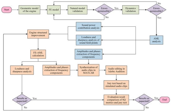
Figure 3.
Flowchart of sound quality SQ evaluation, improvement, and jury test procedures of the diesel engine.
The green process steps are the engine model validation. The blue process steps are the engine radiated noise analysis. The orange process steps are the engine SQ improvement process.
2. Vibo-Acoustic Analysis Based on Finite Element-Automatically Matched Layer FE-AML Method
The FE model of the engine is in Figure 4.
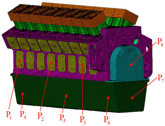
Figure 4.
Finite element FE model of the diesel engine.
The element type and element number of main engine parts are in Table 1. Most of the engine is made of cast iron, except the oil sump which is made of steel. Material parameters are listed in Table 2. To ensure the correctness of the simulated outcomes, both modal and vibrational experiments were conducted for calibration.

Table 1.
Element type and element number of the diesel engine.
Table 2.
Material parameters.
2.1. Modal Validation of the Engine Block
Considering the large size and scale of the engine, a modal experiment was mainly carried out on the engine block. The first ten experimental and simulated natural frequencies are compared in Figure 5. Because the maximum relative error was 4.4%, the accuracy of the block model was deemed acceptable and the vibro-acoustic calculation could be carried out [15].
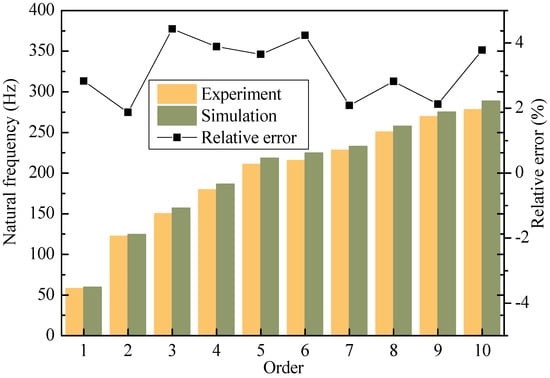
Figure 5.
Contrast between the first ten experimental and simulated natural frequencies of the engine block.
Three modal shapes of the engine block are shown in Figure 6. The first-order mode shows first-order global torsional deformation; the fifth-mode shows second-order global bending deformation; the tenth-mode includes first-order bending deformation of the two symmetrical sides of the engine block.
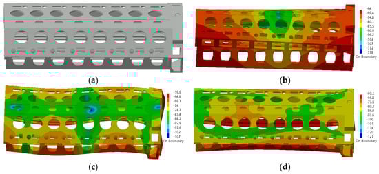
Figure 6.
Modal shapes of the engine block. (a) Original model; (b) First-order mode; (c) Fifth-order mode; (d) Tenth-order mode.
The first 100 modes of the whole diesel engine were then calculated, and 72 were modes of the oil sump. Therefore, the violently vibrating oil sump contributed the most to the vibrations and noise energy of the engine. The oil sump was thus the most important part that needs to be improved.
2.2. Dynamic Validation of Diesel Engine
In this study, four loads were considered, as shown in Figure 7.
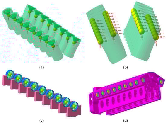
Figure 7.
Four loads considered in this study. (a) Cylinder pressure; (b) Piston side thrust; (c) Main bearing force; (d) Camshaft force.
To verify the vibration results of the entire engine model, eight weak stiffness points (see Figure 4) were chosen to calculate their experimental and simulated average vibration velocities of the engine, referring to the definition of vibration severity. The average vibration velocity was calculated as follows [32]:
where , , and are the numbers of points in three perpendicular directions; and , , and denote the root-mean-squared (RMS) values of velocity in each direction.
The experimental and simulated average vibration velocities of the engine were 38.02 and 40.67 respectively when the engine operating speed was 1066 r/min. The relative error was 6.52%, and thus the accuracy of the FE model and excitation forces was guaranteed, and the calculation process was therefore considered reliable.
2.3. Simulation of Radiated Noise
2.3.1. Automatically Matched Layer AML Method
The AML method is the next-generation version of the perfectly matched layer PML method. It automatically generates the wave-absorbing layer, and the absorption function is renewed for a better performance at a low frequency. This allows the FE models to use smaller elements and therefore achieve a faster calculation speed for exterior acoustics [33].
In this study, the engine-radiated noise was calculated using the AML method as illustrated in Figure 8. The lower threshold of the human auditory frequency range is 20 Hz. Considering that the vibration and noise energy of this low-speed diesel engine is mainly concentrated within 2000 Hz, to reduce the computational time substantially, the frequency range of interest was set as 20–2000 Hz. The acoustic FE mesh was divided with the tetrahedral element. The length of the element was set as 28 mm, because the length of the AML layer element connected to it should satisfy the formula:
where is the sound speed, and is the maximum calculation frequency.
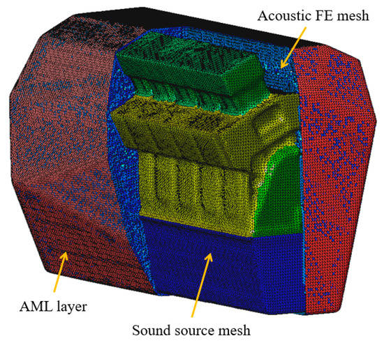
Figure 8.
Acoustic calculation model.
The total number of the acoustic FE element was 2,185,726, and the total node number was 424,015.
2.3.2. Sound Power Contribution of Engine Parts
To compare their radiated sound power contributions within the simulated frequency range, the diesel engine was divided into five parts (see Figure 9).
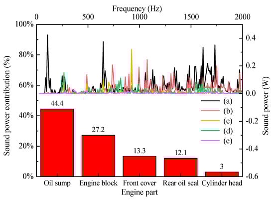
Figure 9.
Sound power spectrum and contribution diagram of five engine parts (A-weighted). (a) Oil sump. (b) Engine block. (c) Front cover. (d) Rear oil seal. (e) Cylinder head.
The upper half of Figure 9 is the A-weighted sound power spectrum of all parts within 20–2000 Hz. The contribution diagram shown in the bottom half was derived from comparing the RMS value of each sound power spectrum. As a result, the oil sump ranked first with 44.4% and the engine block ranked second with 27.2%. The oil sump was determined to be the object for improvement, for the reason that it was shown to be the main source of vibration and noise radiation according to both modal and noise analyses. In addition, the cylinder head contributes the least, so it is not the main noise radiation part from the perspective of sound power.
3. Metrics for Sound Quality SQ Evaluation
3.1. Moore–Glasberg Loudness
In the Moore–Glasberg model, the human auditory frequency range is divided into ERB bands using Cam as the unit [34]:
where is the center frequency value of the n th ERB band.
The specific loudness is calculated as follows:
where is the excitation caused by the sound signals that reach the cochlear filter and its calculation procedure is given in Appendix A, denotes the excitation level at the absolute threshold, is equal to 0.046871, represents the low-level gain of the cochlear amplifier at a specific frequency, and and are both determined based on .
3.2. Sharpness Based on Moore–Glasberg Loudness
The sharpness calculation is mostly based on the specific loudness of the Zwicker model and is standardized as DIN 45692:2009 [22]. The unit of sharpness is acum. Through the center frequency, the ERB number (Cam) can be converted into the critical band rate number (Bark) using Equation (3) and (5). Equation (5) is defined as [19]:
where is the psychoacoustic frequency in Bark.
Swift and Gee [30,31] proposed an approach to predict the sharpness using the specific loudness of the Moore–Glasberg model:
where is a calibration constant, denotes the specific loudness in Cam, is the typical ratio difference between the Zwicker and Moore–Glasberg specific loudness regarding the frequency-spacing scales, represents the psychoacoustic frequency in Cam, and indicates the weighting function defined in DIN 45692:2009 [22]; in addition, the standard weighting function used in this study is indicated as:
4. SQ Analysis and Improvement
4.1. SQ Evaluation of Sound Field Point
The positions of sound field points were determined based on the standard ISO 3744:2010 [35]. Three of them were chosen as an example to study the psychoacoustic characteristics of diesel engine radiated noise. They were separately near the long side of the oil sump, in front of the free end of the engine, and above the cylinder head (see Figure 10).
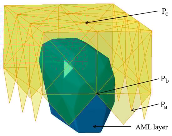
Figure 10.
Positions of three sound field points.
Because the simulated vibro-acoustic frequency range was 20–2000 Hz, when analyzing the specific loudness variation characteristics, the corresponding 1.8–20.5 Cams auditory ERB range was focused on. However, when people are listening to sound, they are affected by the excitation levels of the whole auditory frequency range (1.8–38.9 Cams). In order to be comparative with the jury test results, when referring to total loudness, the specific loudness beyond 1.8–20.5 Cams was calculated according to the auditory masking effect (see Figure 11). The total loudness of , , and for both ears were 345, 304, and 282 sones, respectively.
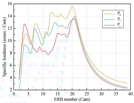
Figure 11.
Specific loudness of three sound field points.
In terms of the different frequency bands of each point, has larger values within 12.2–20.5 Cams, and the peak is located at 20.0 Cams. has larger values within 13.2–20.5 Cams, and the peak is located at 20.5 Cams. has larger values within 3.2–4.8 and 18.9–20.5 Cams, and the peak is located at 20.5 Cams. According to the features above, both and have more noise problems in some of the medium- and the whole high-frequency bands, and have more noise problems in some of the low- and high-frequency bands. Therefore, the high-frequency band should be an area of focus.
From the perspective of the different points in one frequency band, has larger values than other points within 6.0–10.4 and 11.4–20.5 Cams. Because is near the oil sump, it is clear that the oil sump plays a key role in noise energy radiation of the diesel engine. The values of are less than those of the other two points in a wide range of the 6.4–20.5 Cams, and the maximum difference is 6.27 sones/Cam, which appears at 12.8 Cams. Because is near the cylinder head, it can be speculated that the cylinder head is not the main transfer path of the noise energy.
The sharpness calculation results of three sound field points are listed in Table 3. ranks first and is the minimum. It can be presumed again that the oil sump is the main problematic part and the cylinder head is not the main part affecting the SQ of the diesel engine.
Table 3.
Sharpness of three sound field points.
4.2. Improvement Strategy of Oil Sump
According to the outcomes of the vibration and noise and SQ analyses above, the diesel engine demonstrated a worse noise problem within the medium- and high-frequency bands, and the main source was the oil sump. Four of the oil sump’s modal shapes were depicted in Figure 12.
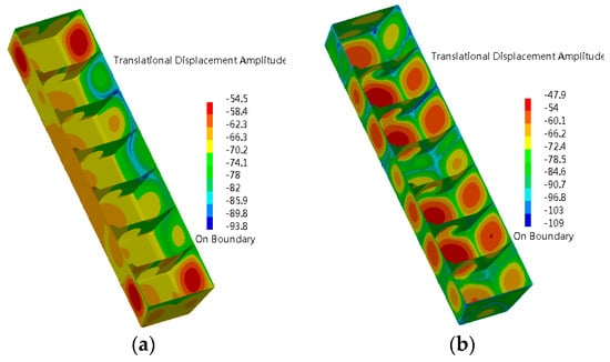
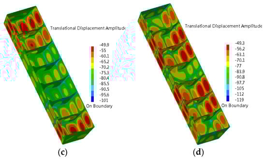
Figure 12.
Four of the oil sump’s modal shapes. (a) 85 Hz. (b) 118 Hz. (c) 180 Hz. (d) 206 Hz.
Because both the side and the bottom of the oil sump are big thin panels, they all have several violent vibration sub-areas that are separated by six partition plates. It can be seen that vibration weakens in the areas near the partition plates. Therefore, the improvement strategy was determined to add several strengthening ribs in the middle of the sub-areas to cut the panels and increase the oil sump’s stiffness as shown in Figure 13. To minimize the impact on the oil sump structure and increase the improvement efficiency, the thickness of the ribs was decided to be 8 mm, identical with the thickness of the oil sump panels. The width of the ribs was determined to be 25 mm according to the width of the connecting part between the engine block and the oil sump.
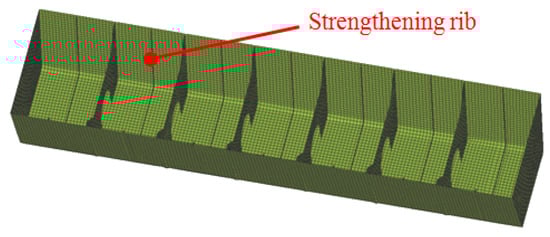
Figure 13.
Structural improvement of oil sump.
4.3. Changes in Radiated Sound Power Level after Improvement
The one-third-octave band diagram of simulated radiated sound power level is in Figure 14. It is clear that more than half of the bands declined, especially the 80, 100, and 125 Hz bands.
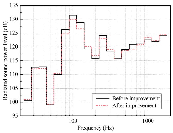
Figure 14.
Diesel engine radiated sound power level before and after improvement.
4.4. SQ Variation of Entire Analyzed Frequency Range after Improvement
To study the SQ improvement effects of the oil sump in detail, was chosen to study the psychoacoustic characteristics of radiated noise. The specific loudness of before and after improvement was calculated based on their SPL data using Moore–Glasberg’s loudness metric, and the outcomes were as depicted in Figure 15. Their total loudness was 324 and 312 sones respectively, so the decrease of total loudness was 12.5 sones after improvement.
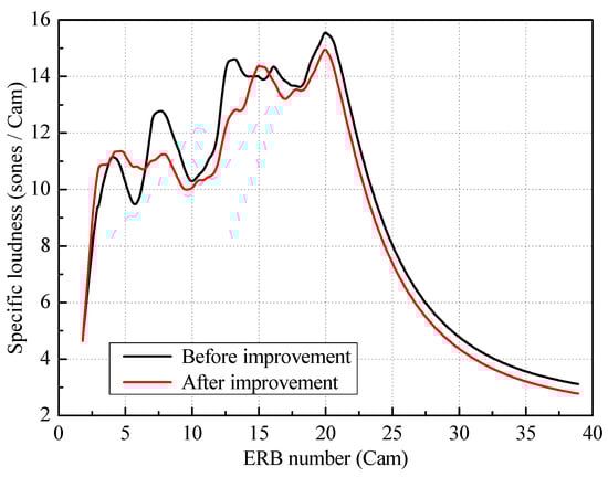
Figure 15.
Specific loudness of sound field point near the oil sump before and after improvement.
In terms of different frequency bands of one oil sump, the original oil sump has larger values within 12.2–20.5 Cams and the peak is 15.6 sones/Cam. The improved oil sump has larger values within 12.2–20.5 Cams and the peak is 15.0 sones/Cam. Both peak points are located at 20.0 Cams. It can be concluded that both oil sumps have larger specific loudness in some of the medium- and the whole high-frequency bands.
From the perspective of both oil sumps in one frequency band, the specific loudness of the improved oil sump declines within the 6.5–14.5 and 15.8–20.5 Cams bands. The biggest decrease is 2.1 sones/Cam, which is located at 12.6 Cams, and the degree of the decrease is 14.4%. It can be speculated that most medium- and high-frequency noises are improved while only some low-frequency noise become worse.
The sharpness of declines from 1.12 to 1.10 acums after improvement. Thus, both the loudness and sharpness of are improved.
4.5. SQ Variation of Four Sub-Bands after Improvement
To further study the psychoacoustic characteristics within different frequency bands, the interested frequency range was divided into four sub-bands, with 4.7 Cams in each sub-band. The central frequencies of the 11.1 and 15.8 Cams are close to the cut-off points of the low-, medium-, and high-frequency bands, respectively (see Table 4). When calculating the specific loudness curve of each sub-band in the whole auditory frequency range, the ERB range beyond the analyzed sub-band is determined by the masking effect (see Figure 16). The loudness and sharpness values of the four sub-bands are listed in Table 5.
Table 4.
Central frequencies of cut-off points of ERB bands.
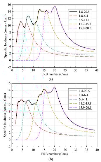
Figure 16.
Specific loudness curves of sub-bands before and after improvement. (a) Before improvement. (b) After improvement.
Table 5.
Loudness and sharpness of sub-bands.
For the loudness, when the ERB range increases, the loudness of sub-bands of both engines rises. Therefore, the medium- and high-frequency bands have more noise problems than the low frequency band. After improvement, the loudness of all bands except the 1.8–6.4 Cams band decreases significantly. The greatest decrement is 14.5 sones within the 11.2–15.8 Cams band. As a result, the noises of most sub-bands were obviously improved, apart from some of the low- frequency bands.
For the sharpness, when the ERB range increases, sharpness of sub-bands of both engines rises. After improvement, sharpness of all sub-bands declines, especially for the 6.5–11.1 Cams band. Hence, it can be speculated that the improvement strategy is effective on the sharpness of the whole analyzed frequency range, particularly the low-frequency band. Because the sharpness of the entire analyzed frequency range cannot be calculated by simply summing the sharpness of the four sub-bands, which differs from the loudness, the improvement effect of the sharpness should take both the sub-bands and the entire analyzed frequency range into consideration at the same time.
Taking both loudness and sharpness into account, the improvement effects of four sub-bands arranged in descending order are 6.5–11.1, 11.2–15.8, 15.9–20.5, and 1.8–6.4 Cams in turn. That means the majority of engine noise was improved in SQ.
To study the change laws in more detail, the analyzed frequency range can be divided into several sub-bands to seek for the problematic frequency band. According to the above analysis, after improvement, the loudness and sharpness of the whole analyzed frequency range and four sub-bands were both improved. In addition, it can be seen that conducting a numerical simulation in advance is important in the development of a diesel engine. For diesel engine noise, making use of the loudness and sharpness, which consider the actual listening experience, can reflect the true impact that noise has on human subjects.
5. Subjective Evaluation of SQ
5.1. Test Samples and Environment
Because the SQ evaluation was based on human auditory perception, to verify the improvement effect and psychoacoustic analysis results of a diesel engine during the simulation stage, 10 audio clips from field point before and after improvement were synthesized for a subjective evaluation. The audio clips were generated in the MATLAB based on the amplitudes and phases of the frequency components derived during the AML analysis. The superposition of the cosine function of each frequency component , with the corresponding angular phase shift and amplitude generates the time-domain sound pressure signal of the noises as:
where is the number of components in the interested frequency range [2].
All the audio clips lasted 5 s. Two of them were audio clips of the entire interested frequency range of sound field point before and after improvement, and were named audio A and audio B, respectively. Eight other audio clips were noise of the four sub-bands of sound field point before and after improvement.
The temperature of the test room was approximately 27 °C, and the humidity was near 41%. The AWSPL of the background noise was about 33 dB(A). Eighteen males and seven females were invited to take part in the jury test. They were university students and teachers (from 22 to 45 years old) majoring in engine or vehicle acoustics and with normal hearing. The test equipment consists of a computer, an amplifier, and a headphone, as illustrated in Figure 17.
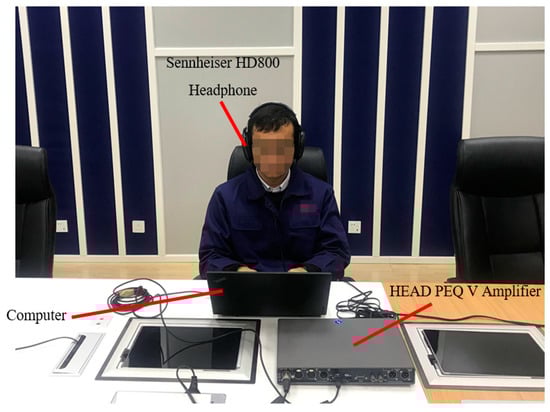
Figure 17.
The test equipment.
5.2. Jury Test of Diesel Engine SQ
Because the total loudness of certain frequency band is a summation of the specific loudness over the band, the audio clips of the sub-bands have much smaller loudness values than audio clips A and B. If they are evaluated together during the same test, the subjective rating scores of sub-band audio clips may vary within a narrow range. To avoid this, the jury test was divided into two experiments, and their interactive test interfaces were as shown in Figure 18.
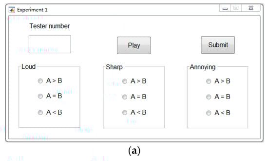
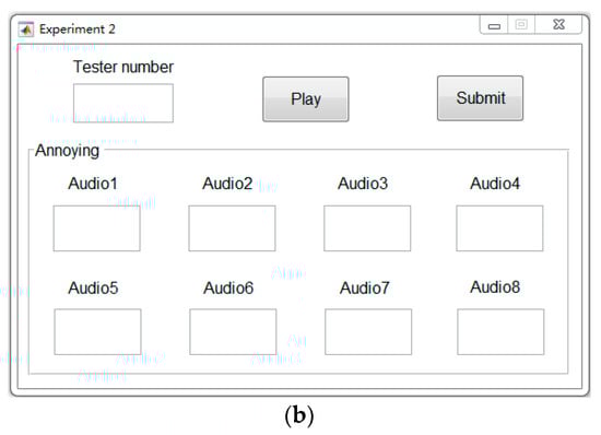
Figure 18.
Interactive interfaces of two experiments. (a) Interactive interface of audio clips A and B. (b) Interactive interface of sub-band audio clips.
The testers were told to type their ID into the tester number blank and click the play button to listen to the audio clips. After hearing and grading the clips, they were instructed to click the Submit button, and the results were saved in an Excel spreadsheet. Because the original levels were too loud for people, the sound volume was adjusted to a level acceptable to testers and kept unchanged during the whole jury test procedure. The relationship of loudness and sharpness between different audio clips has not changed, so the jury test is effective.
The first experiment aimed to compare the loudness, sharpness, and level of annoyance of audio clips A and B using the paired comparison (PC) method [36]. Audio clips A and B were combined with an interval of 1 s of no sound, and the combination was repeated three times with a 5 s interval of no sound between each combination in Adobe Audition software. Twenty-three out of twenty-five people had the same opinion that audio clip A was louder, sharper, and more annoying than audio clip B. These results are consistent with the previous simulation analysis provided in Section 4.3, and the improvement effect was further proved.
The second experiment was rating the eight audio clips of the sub-bands. To minimize the influence of personal preference, the anchored semantic differential (ASD) method [37] with five grades of annoyance semantic meaning in this study (see Table 6) was adopted [6]. When performing the ASD method, an anchor signal selected from the noise samples was required. According to Table 5, the audio clip of the 11.2–15.8 Cams after improvement has intermediate values and was determined as the anchor noise. Its evaluation score was defined as 3 points.
Table 6.
Rating scale definitions of subjective annoying feelings.
The audio clips for the subjective rating in the second experiment were all 11 s long. Each clip was sequentially combined with 5 s of the anchor signal, 1 s of no sound, and 5 s of one of the eight sub-band audio clips. There was 5 s of no sound between each combination. The playback order had no limit, but each audio number corresponding to a specific audio clip was determined in advance.
5.3. Subjective Evaluation Analysis
The sub-band noise results were analyzed using IBM SPSS Statistics software. Kendall’s coefficient was used to indicate agreement among testers. The results of three testers were removed because their Kendall coefficients were lower than 0.7. The average rating scores of the remaining twenty-two testers are listed in Table 7.
Table 7.
Subjective annoyance results of sub-band audio clips.
For the same oil sump, the level of annoyance rises as the ERB range increases. After improvement, the annoyance of all sub-bands declines, especially the medium-, high-, and some of low-frequency bands. That is in accordance with the simulation results illustrated in Section 4.4. Thus, the method for adding strengthening ribs to the oil sump is effective.
The Pearson’s correlation coefficients between the subjective annoyance and psychoacoustic metrics were 0.87 (loudness) and 0.80 (sharpness). Their regression is plotted in Figure 19. It can be seen that both metrics have a strong correlation with the subjective annoyance perception.
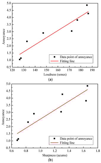
Figure 19.
Analysis results of regression between SQ metrics and annoyance. (a) Correlation between loudness and annoyance. (b) Correlation between sharpness and annoyance.
6. Conclusions
The Moore–Glasberg loudness model divides the human auditory frequency range more finely than the Zwicker loudness model when calculating the excitation level. It is thus more suitable for the narrow bands described herein. Both the Moore–Glasberg loudness and the sharpness based on it reflect real auditory sensations of human subjects. It is therefore more reasonable and reliable to use the loudness and sharpness to analyze the radiated noise of a 16 V diesel engine than the traditional AWSPL and sound power metrics.
According to the structure, acoustics, and SQ analysis results, the oil sump is the main noise radiation source of an engine. Therefore, the variation laws of the Moore–Glasberg loudness and sharpness caused by the change in structure of the oil sump were analyzed. After improvement, the loudness and sharpness of 20–2000 Hz frequency range decreased by 3.9% and 1.8%, respectively.
To compare the improvement effects before and after improvement in more detail, the frequency range of interest was divided into four sub-bands, representing the low-, medium-, and high-frequency bands. In the light of reductions of four sub-bands on both loudness and sharpness, it could be concluded that all sub-bands except the 1.8–6.4 Cams band were obviously improved.
To further verify the results of the simulation analysis, a subjective evaluation was conducted by synthesizing the noises using the amplitudes and phases of the frequency components derived in the AML analysis. Accounting for the difference of loudness among the audio clips, the jury test consisted of two experiments. In view of the subjective grading results, after improvement, the feeling of sharpness, loudness, and annoyance of both the whole interested frequency range and four sub-bands were improved. It is consistent with the conclusions derived in the simulation stage. Moreover, according to the regression of the subjective rating scores and the loudness and sharpness values, both loudness and sharpness have strong correlations with the annoyance perception.
In conclusion, the method of analyzing, improving, and evaluating the SQ of the diesel engine in the simulation stage, proposed in this paper, is feasible and effective.
Author Contributions
Conceptualization, Z.Y.; Supervision, H.F.; Validation, B.M.; Writing—review and editing, A.A.A.K. All authors have read and agreed to the published version of the manuscript.
Funding
This research received no external funding.
Acknowledgments
We would like to thank the engineers at the Shanghai Marine Diesel Engine Research Institute for providing assistance with diesel engine tests.
Conflicts of Interest
The authors declare no conflict of interest.
Abbreviations
| AWSPL | A-weighted sound pressure level |
| SQ | Sound quality |
| FE | Finite element |
| AML | Automatically matched layer |
| SPL | Sound pressure level |
| NVH | Noise, vibration and harshness |
| ERB | Equivalent rectangular bandwidth |
| ASD | Anchored semantic differential |
Appendix A
According to the standard ANSI S3.4-2007, the transfer functions of the human ear are shown in Figure A1. The cochlea in the inner ear can be assumed as an array of bandpass auditory filters with overlapping passbands. The length of each auditory filter is calculated as:
The input excitation is obtained by adding the power spectrum up in one ERB band:
where represents the reference sound pressure Pa, is sound pressure, is a weighting function calculated according to:
where , , is the frequency value of a frequency component in the range.

Figure A1.
Transfer functions of the human ear.
For one auditory filter, the output excitation is the sum of response to each input component:
where is the excitation produced by a 1000 Hz sinusoid at 0 dB SPL (free field, frontal incidence) at the output of the auditory filter centered at 1000 Hz. The shape of the filter is same as Equation (A2) but has different parameter values:
where is the corresponding calculated in Equation (A2).
References
- Liu, H.; Zhang, J.; Guo, P.; Bi, F.; Yu, H.; Ni, G. Sound quality prediction for engine-radiated noise. Mech. Syst. Signal Process. 2015, 56, 277–287. [Google Scholar] [CrossRef]
- Duvigneau, F.; Liefold, S.; Höchstetter, M.; Verhey, J.L.; Gabbert, U. Analysis of simulated engine sounds using a psychoacoustic model. J. Sound Vib. 2016, 366, 544–555. [Google Scholar] [CrossRef]
- Liang, K.; Zhao, H. Automatic evaluation of internal combustion engine noise based on an auditory model. Shock Vib. 2019, 2019, 1–9. [Google Scholar] [CrossRef]
- Huang, H.B.; Li, R.X.; Yang, M.L.; Lim, T.C.; Ding, W.P. Evaluation of vehicle interior sound quality using a continuous restricted Boltzmann machine-based DBN. Mech. Syst. Signal Process. 2017, 84, 245–267. [Google Scholar] [CrossRef]
- Xing, Y.; Wang, Y.; Shi, L.; Guo, H.; Chen, H. Sound quality recognition using optimal wavelet-packet transform and artificial neural network methods. Mech. Syst. Signal Process. 2016, 66, 875–892. [Google Scholar] [CrossRef]
- Wang, Y.; Shen, G.; Xing, Y. A sound quality model for objective synthesis evaluation of vehicle interior noise based on artificial neural network. Mech. Syst. Signal Process. 2014, 45, 255–266. [Google Scholar] [CrossRef]
- Huang, H.B.; Wu, J.H.; Huang, X.R.; Yang, M.L.; Ding, W.P. The development of a deep neural network and its application to evaluating the interior sound quality of pure electric vehicles. Mech. Syst. Signal Process. 2019, 120, 98–116. [Google Scholar] [CrossRef]
- Zheng, X.; Dai, W.; Qiu, Y.; Hao, Z. Prediction and energy contribution analysis of interior noise in a high-speed train based on modified energy finite element analysis. Mech. Syst. Signal Process. 2019, 126, 439–457. [Google Scholar] [CrossRef]
- Ishibashi, M.; Preis, A.; Satoh, F.; Tachibana, H. Relationships between arithmetic averages of sound pressure level calculated in octave bands and Zwicker’s loudness level. Appl. Acoust. 2006, 67, 720–730. [Google Scholar] [CrossRef]
- Yoon, K.; Gwak, D.Y.; Chun, C.; Seong, Y.; Hong, J.; Lee, S. Analysis of frequency dependence on short-term annoyance of conventional railway noise using sound quality metrics in a laboratory context. Appl. Acoust. 2018, 138, 121–132. [Google Scholar] [CrossRef]
- Luo, L.; Zheng, X.; Hao, Z.-Y.; Dai, W.-Q.; Yang, W.-Y. Sound quality evaluation of high-speed train interior noise by adaptive Moore loudness algorithm. J. Zhejiang Univ. Sci. A 2017, 18, 690–703. [Google Scholar] [CrossRef]
- Yan, L.; Jiang, W. Research on the procedure for analyzing the sound quality contribution of sound sources and its application. Appl. Acoust. 2014, 79, 75–80. [Google Scholar] [CrossRef]
- Valverde, N.; Ribeiro, R.; Henriques, E.; Fontul, M. Psychoacoustic metrics for assessing the quality of automotive HMIs’ impulsive sounds. Appl. Acoust. 2018, 137, 108–120. [Google Scholar] [CrossRef]
- Kook, J.; Koo, K.; Hyun, J.; Jensen, J.S.; Wang, S. Acoustical topology optimization for Zwicker’s loudness model—Application to noise barriers. Comput. Methods Appl. Mech. Eng. 2012, 237, 130–151. [Google Scholar] [CrossRef]
- Mao, J.; Hao, Z.-Y.; Jing, G.-X.; Zheng, X.; Liu, C. Sound quality improvement for a four-cylinder diesel engine by the block structure optimization. Appl. Acoust. 2013, 74, 150–159. [Google Scholar] [CrossRef]
- Mao, J.; Hao, Z.-Y.; Zheng, K.; Jing, G.-X. Experimental validation of sound quality simulation and optimization of a four-cylinder diesel engine. J. Zhejiang Univ. Sci. A 2013, 14, 341–352. [Google Scholar] [CrossRef]
- Fan, R.; Meng, G.; Su, Z.Q. Research on the interior noise reduction of an elastic cavity by the multipoint panel acoustic contribution method based on moore–glasberg loudness model. J. Vib. Acoust. 2014, 136, 061004. [Google Scholar] [CrossRef]
- Moore, B.C.J.; Glasberg, B.R.; Baer, T. A model for the prediction of thresholds, loudness, and partial loudness. J. Audio Eng. Soc. 1997, 45, 224–240. [Google Scholar]
- Fastl, H.; Zwicker, E. Psychoacoustics: Facts and Models, 3rd ed.; Springer Press: Berlin/Heidelberg, Germany, 2007. [Google Scholar]
- Smith, J.; Abel, J. Bark and ERB bilinear transforms. IEEE Trans. Speech Audio Process. 1999, 7, 697–708. [Google Scholar] [CrossRef]
- ANSI. ANSI S3.4-2007 Procedure for the Computation of Loudness of Steady Sounds; American National Standards Institute: Washington, DC, USA, 2007. [Google Scholar]
- DIN. DIN 45692-2009-08 Measurement Technique for the Simulation of the Auditory Sensation of Sharpness; Deutsches Institut für Normung: Berlin, Germany, 2009. [Google Scholar]
- Huang, H.B.; Li, R.X.; Huang, X.R.; Yang, M.L.; Ding, W.P. Sound quality evaluation of vehicle suspension shock absorber rattling noise based on the Wigner-Ville distribution. Appl. Acoust. 2015, 100, 18–25. [Google Scholar] [CrossRef]
- Morel, J.; Marquis-Favre, C.; Gille, L.-A. Noise annoyance assessment of various urban road vehicle pass-by noises in isolation and combined with industrial noise: A laboratory study. Appl. Acoust. 2016, 101, 47–57. [Google Scholar] [CrossRef]
- Xu, Z.; Xia, X.; Lai, S.; He, Z. Improvement of interior sound quality for passenger car based on optimization of sound pressure distribution in low frequency. Appl. Acoust. 2018, 130, 43–51. [Google Scholar] [CrossRef]
- Freitas, E.F.; Martins, F.F.; Oliveira, A.; Segundo, I.R.; Torres, H. Traffic noise and pavement distresses: Modelling and assessment of input parameters influence through data mining techniques. Appl. Acoust. 2018, 138, 147–155. [Google Scholar] [CrossRef]
- Zhang, J.; Xia, S.; Ye, S.; Xu, B.; Zhu, S.; Xiang, J.; Tang, H. Experimental investigation on the sharpness reduction of an axial piston pump with reinforced shell. Appl. Acoust. 2018, 142, 36–43. [Google Scholar] [CrossRef]
- Fang, Y.; Zhang, T. Sound quality investigation and improvement of an electric powertrain for electric vehicles. IEEE Trans. Ind. Electron. 2018, 65, 1149–1157. [Google Scholar] [CrossRef]
- Zhang, J.; Xia, S.; Ye, S.; Xu, B.; Zhu, S.; Xiang, J.; Tang, H. Sound quality evaluation and prediction for the emitted noise of axial piston pumps. Appl. Acoust. 2019, 145, 27–40. [Google Scholar] [CrossRef]
- Swift, S.H.; Gee, K.L. Implementing sharpness using specific loudness calculated from the “Procedure for the Computation of Loudness of Steady Sounds”. In Proceedings of the 173rd Meeting of Acoustical Society of America and 8th Forum Acusticum, Boston, MA, USA, 25–29 June 2017; Volume 30. [Google Scholar]
- Swift, S.H.; Gee, K.L. Extending sharpness calculation for an alternative loudness metric input. J. Acoust. Soc. Am. 2017, 142, 549–554. [Google Scholar] [CrossRef]
- ISO. ISO 2041-2018 Mechanical Vibration, Shock and Condition Monitoring-Vocabulary; International Organization for Standardization: Geneva, Switzerland, 2018. [Google Scholar]
- Singer, I.; Turkel, E. A perfectly matched layer for the Helmholtz equation in a semi-infinite strip. J. Comput. Phys. 2004, 201, 439–465. [Google Scholar] [CrossRef]
- Moore, B.C.J. Development and current status of the “Cambridge” loudness models. Trends Hear. 2014, 18, 1–29. [Google Scholar] [CrossRef]
- ISO. ISO 3744-2010 Acoustics—Determination of Sound Power Levels and Sound Energy Levels of Noise Sources Using Sound Pressure—Engineering Methods for an Essentially Free Field over a Reflecting Plane; International Organization for Standardization: Geneva, Switzerland, 2010. [Google Scholar]
- David, H.A. The Method of Paired Comparisons; Oxford Press: New York, NY, USA, 1988. [Google Scholar]
- Mao, D.X.; Zhang, B.L. Performance of semantic differential method with an anchor stimulus in subjective sound quality evaluation. Tech. Acoust. 2006, 25, 560–567. [Google Scholar]
© 2020 by the authors. Licensee MDPI, Basel, Switzerland. This article is an open access article distributed under the terms and conditions of the Creative Commons Attribution (CC BY) license (http://creativecommons.org/licenses/by/4.0/).