Article

A Data-Driven Method with Feature Enhancement and Adaptive Optimization for Lithium-Ion Battery Remaining Useful Life Prediction

1
School of Computer Science and Engineering, Central South University, Changsha 410083, China
2
School of Automation, Central South University, Changsha 410083, China
3
College of Automotive and Mechanical Engineering, Changsha University of Science & Technology, Changsha 410114, China
*
Author to whom correspondence should be addressed.
Energies 2020, 13(3), 752; https://doi.org/10.3390/en13030752
Submission received: 31 December 2019 / Revised: 23 January 2020 / Accepted: 4 February 2020 / Published: 8 February 2020
(This article belongs to the Special Issue Artificial Intelligence Applications to Energy Systems)

Abstract

:
Data-driven methods are widely applied to predict the remaining useful life (RUL) of lithium-ion batteries, but they generally suffer from two limitations: (i) the potentials of features are not fully exploited, and (ii) the parameters of the prediction model are difficult to determine. To address this challenge, this paper proposes a new data-driven method using feature enhancement and adaptive optimization. First, the features of battery aging are extracted online. Then, the feature enhancement technologies, including the box-cox transformation and the time window processing, are used to fully exploit the potential of features. The box-cox transformation can improve the correlation between the features and the aging status of the battery, and the time window processing can effectively exploit the time information hidden in the historical features sequence. Based on this, gradient boosting decision trees are used to establish the RUL prediction model, and the particle swarm optimization is used to adaptively optimize the model parameters. This method was applied on actual lithium-ion battery degradation data, and the experimental results show that the proposed model is superior to traditional prediction methods in terms of accuracy.

Graphical Abstract

1. Introduction

With the global energy crisis and environmental pollution problems intensifying, electric vehicles have been rapidly promoted by countries around the world for their advantages of high efficiency, energy saving, low noise and zero emissions [1,2]. Due to the high energy density, high cell voltage, low self-discharge rate and long life, lithium-ion batteries are widely used in power systems of electric vehicles [3,4]. But with degradation, the battery will face many issues (capacity degradation, internal resistance increase, etc.), which will have a significant impact on the mileage and safety of electric vehicles. The remaining useful life (RUL) can indicate the remaining time before the battery needs to be replaced, and an alarm can be issued before the fault reaches a critical level, so that timely maintenance can be performed to prevent malfunction, or even catastrophic failures [5,6]. Therefore, the prediction of RUL has become a research hotspot in the prognostics and health management of the lithium-ion battery, and it is also one of the important goals for the battery management systems of electric vehicles [7].
In recent years, many methods have been proposed for battery RUL prediction, which can be roughly divided into two categories: model-based methods and data-driven methods [8]. The model-based methods predict battery RUL based on a physical model or a mathematical model [9]. Remmlinger et al. [10] improved the second-order RC equivalent circuit model, and then combined special load signals (transient voltage, current during engine start-up) and the linear least squares method to obtain the internal resistance. Based on the internal resistance, the battery’s aging status was captured. Ramadass et al. [11] proposed a battery decay model based on electrochemical principles. In this model, the growth of a solid–electrolyte interface film was considered, which is associated with capacity fading and active lithium-ion consumption. In addition, many empirical model-based methods have also been developed. Xian et al. [12] employed the verhulst model, particle swarm optimization, and particle filter to estimate the RUL of batteries. He et al. [13] established an empirical model based on the physical degradation behavior of lithium-ion batteries. They initialized the model parameters by the Dempster–Shafer theory, and updated the model parameters using the Bayesian Monte Carlo method. The model-based methods can approximately reflect the dynamic and static characteristics of the battery, but choosing a suitable physical or mathematical model requires a large amount of domain knowledge [14]. Moreover, as the operating conditions (e.g., power, temperature) change, the complex coupled nonlinear partial differential equations need to be frequently solved [15], and the simplified methods of this solution process are difficult to implement [16,17]. These factors limit the application of model-based methods.
The data-driven methods have been popular for battery RUL prediction recently. Unlike the model-based methods, the data-driven methods are based on large numbers of data, where the deep understanding of electrochemical principles is not necessary [18]. It mainly includes the support vector machine [19,20,21], neural network [22,23], Bayesian method [24,25], random forest [26] and so on. For data-driven methods, the effectiveness of features and the performance of regression algorithms can greatly affect the accuracy of the RUL prediction, so they have attracted the attention of many researchers.
In order to improve the accuracy of RUL predictions, various features have been explored to capture the degradation of batteries. Goebel et al. [7] used the impedance in the electrode-electrolyte interface as a feature variable to predict the RUL of the battery. Lee et al. [27] used open-circuit voltage (OCV) as a feature to estimate the state-of-charge and the capacity. Considering that both internal resistance and OCV are difficult to measure, some studies tried to capture the aging status of batteries through external parameters. Wu et al. [23] put the voltage curves during the whole constant current charge into the neural network model, and established the mapping relationship between the voltage curve shape and the RUL. Liu et al. [28] extracted the time interval of the discharge voltage difference for predicting the RUL of the satellite battery. Widodo et al. [29] used the sample entropy of the discharge voltage as a feature to reflect the health of the battery.
It is worth noting that the existing studies mainly focus on finding new features with superior performance, but ignore exploiting the feature potential. In fact, if the potential of features can be fully exploited using feature enhancement technologies, the accuracy of RUL prediction can be further improved. Specifically, due to the internal and external factors, the degradation process of the battery is extremely complicated [30,31]. As a result, the relationship between features and RUL is significantly non-linear, which increases the difficulty of RUL prediction. If the correlation between features and RUL can be improved, the accuracy of RUL prediction can be improved. In addition, the degradation of the battery is a continuous process, and the historical cycle states of the battery are critical to the current RUL prediction. If the time information hidden in the historical cycles can be effectively exploited, the accuracy of the RUL prediction can be improved.
In order to improve the accuracy of RUL prediction, many studies tried to use advanced machine learning algorithms to establish the mapping relationship between features and RUL. Wu et al. [23] combined a feed forward neural network and importance sampling to learn the relationship between the RUL and charge curves. This algorithm can handle the nonlinearity of a lithium-ion battery well, but the neural network requires a large amount of training data, and it is easy to fall into a local minimum during the solution process. Patil et al. [21] proposed a multistage support vector machine approach for RUL prediction, where the classification model provided a gross estimation and the regression model was used for accurate prediction, which can reduce the computational load, but the performance of support vector machine depends on the choice of kernel functions. Razavi-Far et al. [26] used battery capacity as the feature and used random forest to predict RUL. However, due to the randomness of the training process, it is difficult for the random forest method to obtain stable prediction results. In recent years, the gradient boosting decision tree (GBDT) has developed rapidly. As a tree-based ensemble algorithm, GBDT only requires very little data and can fit a complex nonlinear relationship. Studies have shown that GBDT has considerable advantages over traditional statistical methods [32]. In our previous work, GBDT has been successfully applied in the battery RUL prediction. However, the disadvantage of GBDT is that its parameter selection is difficult. Some parameters (the number of trees, the learning rate, the number of leaf nodes) determine the structure and training method of the model, which affects the prediction performance. In order to fully realize the potential of GBDT, it is necessary to develop appropriate strategies to determine the parameters.
Inspired by the above discussion, this paper presents a new data-driven method for battery RUL prediction. We first extract the raw features online from the voltage signal that reflect the aging state of the battery. Then, the feature enhancement technologies, including the box-cox transformation and the time window processing, are used to fully exploit the potential of features, where the box-cox transformation is used to enhance the correlation between features and RUL, and the time window processing is used to deeply exploit the time information hidden in the sequence of historical cycles. In addition, based on the extracted features, GBDT with strong regression ability is used to establish the RUL prediction model, and the particle swarm optimization (PSO) is adopted to adaptively optimize the model parameters.
In our previous work [33], the time window and GBDT were proposed for the RUL prediction of lithium-ion batteries. Compared with the conference version, this paper provides three new contributions:
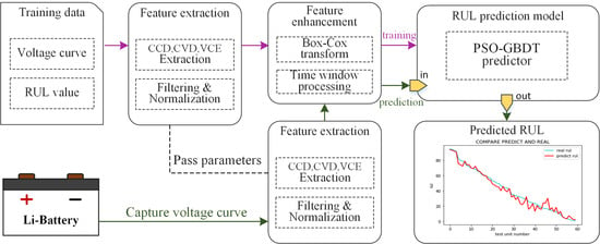
  • Duration of constant current mode, duration of constant voltage mode and energy of discharge voltage are extracted as features so that we can capture the degradation of the battery from various angles.
  • The feature enhancement technologies including the box-cox transformation and the time window processing are proposed to fully exploit the potential of features.
  • PSO is introduced to adaptively find the optimal parameters of GBDT, which improves the accuracy and stability of RUL prediction.
The remainder of this paper is organized as follows. In Section 2, we introduce the proposed RUL prediction framework and related technical algorithms. In Section 3, the battery data set is introduced. Additionally, the validity of the raw features and the box-cox transformation is presented. In Section 4, the optimization process of PSO is shown, and experiments in various cases prove the accuracy and reliability of the proposed method. The conclusion and prospects are given in Section 5.

2. Proposed Approach

2.1. Framework

The data-driven RUL prediction method proposed in this paper is shown in Figure 1. The method uses features extracted from the real-time voltage curves of the battery to predict the RUL, which is suitable for online scenes. In addition, the feature enhancement technologies and the machine learning algorithm with powerful regression capabilities are used. This method can perform accurate RUL prediction, and it contains two steps: a training step and a prediction step.
In the training step, duration of constant current mode ( C C D ), duration of constant voltage mode ( C V D ) and energy of discharge voltage ( V C E ) are extracted from the training data as raw features. After filtering and normalizing the extracted features, the feature enhancement technologies are used to fully exploit the potential of features, including the box-cox transformation and the time window processing. These data are then used to train the PSO-GBDT model. During the training process, the optimal parameters of the model are adaptively optimized, including the number of trees M, learning rate ξ and the number of leaf nodes N.
In the prediction step, C C D , C V D and V C E are extracted online from the voltage curves of the battery to be measured. After the same filtering and feature enhancement operations as in the training step (using the same parameters), the final feature data is fed into the trained PSO-GBDT model to obtain the predicted value of RUL.

2.2. Raw Feature Extraction and Correlation Analysis

Considering that the internal characteristics change during battery aging, and this change can be reflected by external parameters, we extract C C D , C V D and V C E from the voltage curves as the raw features to capture the aging status of the battery, where the battery is charged with a constant current-constant voltage (CC-CV) mode [34] and discharged with a constant current (CC) mode.
C C D is the duration of CC charging mode, which is a direct indicator of the battery’s charging capacity in CC mode, and it reflects the polarization of the battery to a certain extent. C V D is the duration of constant voltage (CV) charging mode, and its size can reflect the difficulty level of the lithium-ion intercalation process [31]. V C E is the measure of signal strength of the discharge voltage signal over time, and is calculated by
V C E = + x t 2 d t
where x is the voltage signal and t is time.
Figure 2 shows the extraction methods of C C D , C V D and V C E .
To verify the validity of the raw features, in this work, the Pearson correlation analysis [35] is used to calculate the correlation between the extracted features and actual RUL, and it is calculated by
C o r r = i = 1 n y i y ¯ R U L i R U L ¯ i = 1 n y i y ¯ 2 i = 1 n R U L i R U L ¯ 2
where y i and R U L i are the feature value and RUL value of the i t h observation sample. n is the number of the samples. The closer the Pearson correlation is to 1 or −1, the stronger the correlation. The closer the Pearson correlation is to 0, the weaker the correlation.

2.3. Box–Cox Transformation and Time Window Processing

The raw features, such as C C D , C V D and V C E , can reflect the aging of the battery through its own changing trend. However, due to the complexity of the underlying degradation process of the battery, the raw features and the aging status do not have a complete linear relationship, which increases the difficulty in predicting RUL. Therefore, in this paper, we use the box-cox transformation to enhance the linear relationship between the raw features and RUL and improve the prediction performance of the features.
The box-cox transformation is a generalized power transform method, which can improve the additivity, normality and homoscedasticity of raw features.
Let y = y 1 , y 2 , , y n be the raw feature to be converted by the box-cox transformation; say, v c e = v c e 1 , v c e 2 , , v c e n . Mathematically, the box-cox transformation takes the following form
y λ = y λ 1 λ , λ 0 ln y , λ = 0
where λ is the transformation parameter to be identified, and different λ s correspond to different transformations. Note that the transformation is only valid for y i > 0 , i = 1 , 2 , , n , and modifications have to be made when negative raw features are present.
In the box-cox transformation, parameter λ needs to be determined to ensure the usual assumptions for linear model hold, which is y λ N X β , σ 2 I and can be expressed as
y λ = X β + e e N 0 , σ 2 I
where X is the regression independent variable, which in this paper refers to the RUL; β is the set of parameters associated with the y λ ; and e = e 1 , e 2 , , e n is the error term.
We use the maximum likelihood (ML) method [36] to determine λ . Since y λ N X β , σ 2 I , for a fixed λ , the likelihood function of β and σ 2 is
L β , σ 2 = 1 2 π w 2 exp 1 2 σ 2 y λ X β y λ X β J
where J is the transformed Jacobi determinant
J = i = 1 n d y i λ d y i = i = 1 n y i λ 1
Taking the partial derivatives of Equation (5) with respect to β and σ 2 , and setting each of the resulting equations to zero yields, we can get
β λ = X X 1 X y λ
σ ^ 2 λ = y λ I X X X 1 X n
The log-likelihood function can be expressed as
ln L λ = n 2 ln z λ I X X X 1 X z λ
where
z λ = Z 1 λ , , Z n λ = y λ J 1 n
Z i λ = y i λ i = 1 n y i λ 1 n , λ 0 ln y i i = 1 n y i 1 n λ = 0
In order to maximize Equation (5), the Newton’s method is used to find the most suitable λ ^ , and then the corresponding β ^ can be obtained by Equation (7).
In this work, we perform the box-cox transformation on C C D , C V D and V C E to get corresponding C C D b c t , C V D b c t and V C E b c t , and their transformation parameters are λ c c d , λ c v d and λ v c e .
To deeply exploit the time information hidden in the historical feature sequence, time window processing is used. In this process, multiple features from consecutive cycles are packaged into a window of size S, and the RUL label of each window is the RUL value of the latest unit in it.
Let C C D b c t ( k ) , C V D b c t ( k ) and V C E b c t ( k ) be the features of the k t h cycle; then, a data set D containing n cycles can be expressed as
D = w 1 , y 1 , , w n s + 1 , y n s + 1
where w i is the i t h window, as follows:
w i = C C D b c t i , , C C D b c t i + s 1 C V D b c t i , , C V D b c t i + s 1 V C E b c t i , , V C E b c t i + s 1
and y i is the RUL of the i t h window.

2.4. Gradient Boosting Decision Trees (GBDT) for RUL Prediction

In this paper, GBDT is used to establish the RUL prediction model. As an ensemble learning method, GBDT uses multiple decision trees as base learners, and each leaf on a tree has a real score. GBDT gets the final score by adding predictions of all the trees, and for an input w i , the RUL prediction result can be expressed as
R U L i = m = 1 M g m w i
where, M is the number of decision trees. g m is the m t h tree, which divides the input into J disjoint regions R 1 m , R 2 m , , R j m , and each region corresponds to a prediction value b j m . g m is expressed as follows
g m w = j = 1 J b j m I w
I w = 1 , w R j m 0 , w R j m
GBDT uses the gradient boosting strategy for training. It sequentially generates multiple base models from a weighted version of the training data to strategically find the best combination of decision trees. In the boosting process, each additional base model is aimed to correct the residuals made by its previous base models, and the updating equation is as follows
f m w = f m 1 w + ξ · ρ m g m w
ρ m = arg min ρ i = 1 n L R U L i , f m 1 w + ξ · ρ g m w i
where n is the number of training samples; the loss function L is the squared error function; and ρ m is the gradient descent step size of g m ( w ) . In addition, to prevent overfitting, GBDT introduces the learning rate ξ to control the contribution of each base model, and ξ 0 , 1 .
GBDT is excellent in terms of regression ability, but as a tree-based ensemble algorithm, the structure and update method of the model has a great impact on its performance, which mainly includes the three parameters of the number of trees M, learning rate ξ and the number of leaf nodes N. Therefore, to ensure the performance of the model, we need to optimize these parameters.
Algorithm 1 The training and optimization process of the PSO-GBDT model.
  • Initialize particle swarm parameters D , P , C 1 , C 2 , ω , and randomly initialize p , v for particles.
  • for j = 1 toQdo
  •  Initialize f 0 x to be a constant, f 0 x = a r g min ρ i = 1 N L y i , ρ .
  • for m = 1 to M do
  •   for i = 1 to n do
  •    Compute the negative gradient
    z i m = σ L y i , f x i σ f x i f = f m 1
  •   end for
  •   Fit a tree g m x to predict the targets z i m from covariates x i for all training data.
  •   Compute a gradient descent step size as
    ρ m = arg min ρ i = 1 n L y i , f m 1 x + ξ · ρ g m x i
  •   Update the model as
    f m x = f m 1 x + ξ · ρ m g m x
  • end for
  •  Get the GBDT f M x and evaluate its performance. Compute the fitness p i d , p g d .
  •  Update each particle as
    v i d k + 1 = ω v i d k + C 1 r a n d ( 0 , 1 ) ( p i d x i d k ) + C 2 r a n d ( 0 , 1 ) ( p g d x i d k )
    x i d k + 1 = x i d k + v i d k
  • end for
  • Output the final PSO-GBDT model.

2.5. Particle Swarm Optimization (PSO) for Model Optimization

In this work, PSO is used to find the optimal combination of these parameters. PSO finds optimal parameters by simulating foraging behavior of birds. Assume that a particle swarm of P particles is flying in D-dimensional space. The current position of particle i is x i = x i 1 , , x i D and the speed is v i = v i 1 , , v i D . p i d = p i 1 , , p i D is the current optimal position of particle i, and p g d = p 1 , , p D is the global optimal position. PSO updates the particle according to the global optimal position and the individual optimal position as follows.
v i d k + 1 = ω v i d k + C 1 r a n d ( 0 , 1 ) ( p i d x i d k ) + C 2 r a n d ( 0 , 1 ) ( p g d x i d k )
x i d k + 1 = x i d k + v i d k
where ω is the inertia factor, d means the dimension number, k is the iteration number and r a n d ( 0 , 1 ) represents a random number between 0 and 1. C 1 and C 2 are the acceleration constants; they usually take the values [0, 4]. Optimized parameters can be obtained after Q iterations. After integrating PSO and GBDT, the training and optimization process of the RUL prediction model is shown in Algorithm 1.

3. Data Description and Feature Analysis

In this section, the battery data set used in the experiments is introduced. Based on the battery data set, the raw features and the box-cox transformation are verified.

3.1. Lithium-Ion Battery Data Set

In this work, in order to verify the proposed method, experiments and analysis were performed on multiple lithium-ion batteries. The battery cycling data were sourced from a publicly available data set, which is provided by Prognostics Center of Excellence (PCoE) at NASA [37]. This data set was collected on several commercially available lithium-ion 18650-sized rechargeable batteries based on NASA’s battery prediction test bed. The test bed contains a power supply, a thermocouple sensor, a programmable DC electronic load, a voltmeter, an environmental chamber, an electrochemical impedance spectrometer and a PXI-based data acquisition system. In the aging experiments, the lithium-ion batteries were cycled in three different modes (charge, discharge and impedance) at specific temperatures (Batteries #5, #6, #7 and #33 were 24 C; Battery #56 was 4 C) to accelerate aging. The charging used CC-CV mode. The batteries were first charged to 4.2 V in 1.5 A CC mode, and then continued to charge in CV mode until the charging current dropped to 20 mA. The discharge used CC mode. The batteries were discharged at the set current (Batteries #5, #6, #7 and #56 were 2 A; Battery #33 was 4 A) until the battery voltage dropped to the threshold (2.7 V, 2.5 V, 2.2 V, 2.0 V and 2.7 V for Batteries #5, #6, #7, #33 and #56, respectively). During the charging and discharging process, the voltage, current, capacity, impedance and temperature of each batteries was collected. When the rated capacity dropped to the threshold (Batteries #5, #6, #7 and #56 were 1.4 Ah; Battery #33 was 1.6 Ah), the batteries reached the end of life (EOL) and the experiments stopped. The number of cycles for Batteries #5, #6, #7, #8, #33 and #56 were 168, 168, 168, 197, and 102, respectively. Table 1 lists the details of these batteries.

3.2. Raw Feature Extraction

As the battery degrades, many irreversible electrochemical changes occur inside the battery (such as the growth of the EIS film), and these changes can be represented by the charging and discharging characteristics of the battery. Figure 3 shows the charging and discharging curves of Battery #6 at different cycles. It can be seen that from Figure 3a that as the number of battery cycles increases, the duration of CC charging mode has a significant downward trend, and the duration of CV charging mode has a significant upward trend. In view of the obvious regularity of the charging voltage curves in geometry, we can extract features from the geometric perspective. From Figure 3b we can see that as the number of battery cycles increases, the discharge voltage at the same moment in each cycle gradually decreases, and the duration of the CC discharge mode gradually decreases. Therefore, the concept of signal energy can be used to extract features from the discharge voltage curves.
According to the method introduced in Section 2.2, we extract C C D , C V D and V C E from Batteries #5, #6 and #7 respectively, and use the sliding window filtering algorithm to filter some obvious outliers. The numerical ranges of these features may be very different, which will have a great impact on the model training. Therefore, the features need to be normalized. In this work, Min-Max normalization is used, which can scale the features to the range of [0, 1]. For the i t h value in the j t h feature sequence, the normalization process is shown in Equation (21).
y i j = x i j min x j max x j min x j
Figure 4 shows the raw features variation of Battery #6. It can be seen that, as discussed above, the C C D and V C E have a significant downward trend as the number of cycles increases. C V D shows a clear upward trend overall. Note that the CV charging mode stops once the current drops to 20 mA. There is a certain error in the measurement of C V D due to the small cut-off current and the noise drift of the current sensor, which causes a local degree of jitter in the C V D curve. Therefore, C C D , C V D and V C E can be used as features to reflect the aging status of the battery. Additionally, it should be noted that even though there may be redundant terms in the selected features, they will not affect the final RUL prediction.

3.3. Correlation Enhancement for Features

In the above discussion, we found through a qualitative analysis that there is a correlation between the raw features and the degree of aging of the batteries. In this section, we use the Pearson correlation to quantitatively calculate the correlation between the raw features and the RUL, and use the box-cox transformation to further improve it.
In this work, we define RUL by using the percentage of the remaining charge-discharge cycles in the total number of cycles. For a battery at N i cycles, RUL is defined as:
R U L = N E O L N i N E O L × 100
According Equation (2), the Pearson correlations between the raw features and RUL of every battery are acquired, as shown in Table 2. It can be seen that the Pearson correlation between C C D , V C E and RUL is close to −1, indicating that they have a strong negative correlation. And the Pearson correlation of C V D and RUL is close to 1, indicating that they have a strong positive correlation.
We use the box-cox transformation to enhance the correlation between features and RUL. Since different transformation parameters λ correspond to different transformation formulas, in order to determine the optimal λ , we use different λ in [−10,10] to transform features and calculate the corresponding Pearson correlations. The optimization process is shown in Figure 5. Note that the optimal transformation parameters for the same feature are slightly different in different batteries, and we chose the mean value as the optimal λ . For C C D , C V D and V C E , the optimal λ are 0.17, 3.3 and −2.8, respectively. We transformed the features based on the optimal λ . Table 2 records the Pearson correlations after the transformation. It can be found that the Pearson correlations of the three features are closer to 1 or −1 than before the transformation, which indicates that the box-cox transformation enhances the correlation between the features and RUL. The transformed features of Battery #6 are shown in Figure 6. It can be seen that the linearity between the features and RUL has been improved, which will promote RUL prediction.

4. Battery RUL Prediction with PSO-GBDT Model

In this section, the proposed RUL prediction method is applied to the NASA data set, and several experiments are designed to verify its effectiveness. The experimental platform is a desktop PC with an Intel Core i7-9700K 3.60-GHz CPU and 16-GB RAM, and the operating system is Windows 10.
In the following validation, the root mean square error (RMSE) is adopted as the key performance indicator (KPI) to evaluate the performance of the proposed method. It is given as:
R M S E = 1 N i = 1 N r r e a l i r ^ i 2
where N is the total number of test samples. r r e a l is the actual RUL, and r ^ is the corresponding prediction value.

4.1. Model Parameter Optimization with PSO

In order to determine important parameters such as the number of trees M, learning rate ξ and the number of leaf nodes N in the proposed RUL prediction model, PSO is used for parameter optimization. We use five particles to form the particle swarm, and randomly initialize their positions (parameters of GBDT) and velocity parameters. In the process of iterative optimization, we use all samples of Batteries #5, #6 and #7 to perform a 5-fold cross validation on the proposed model, and the RMSE results are used to evaluate the fitness of the particles. The iterative optimization process of the PSO-GBDT model is shown in Figure 7. Figure 7a shows the trajectories of the five particles, where the X axis is the number of trees M, the Y axis is the learning rate ξ and the Z axis is the number of leaf nodes N. In the early stage of PSO optimization, a larger velocity inertia coefficient makes the update step of each parameter larger, which is beneficial to initially find the global optimal region of the particle swarm. In the later stage of PSO optimization, the velocity inertia coefficient decreased significantly, and the smaller update step makes each particle gradually approach the global optimal region of the parameter space.
In Figure 7b, five particles continuously record and update their parameters through self-learning and mutual learning between particles. In each iteration, the optimal value of the current iteration is compared with the historical optimal value to continuously update the global optimal value of the particle swarm. Finally, after 60 iterations, the optimization process is stopped. It can be seen that during the PSO optimization process, the average RMSE of the 5-fold cross validation gradually decreases from 2.95 and finally stabilizes to 2.07, which indicates that the adaptive optimization of the parameters by PSO can significantly improve the prediction accuracy of the GBDT model. Based on PSO optimization, the important parameters of the GBDT model are shown in Table 3.

4.2. Experimental Case 1: Single Battery Data

In order to verify the reliability and accuracy of the proposed RUL prediction model, we first applied the PSO-GBDT model to Batteries #5, #6 and #7, respectively. For each battery, we selected 70% of the samples as the training set (117 samples), and selected the remaining 30% of the samples as the test set (51 samples). To generate unbiased samples, the random number generator was used. Note that this method does not require strong battery consistency. Due to the process factors, the three batteries in this experiment have different initial capacities, but this method still works. Figure 8 shows the RUL prediction results for Batteries #5, #6 and #7, where panels (a), (c) and (e) show the RUL prediction values and the corresponding actual values for the three batteries. Panels (b), (d) and (f) are the absolute errors of the prediction results. The RUL prediction values of the three batteries are very close to the actual values, and the absolute errors of most sample points are less than 5%. From Table 4, we can see that the RMSEs of the RUL prediction values for Batteries #5, #6 and #7 are 1.927, 2.496 and 2.142. The small RMSEs also indicate that the proposed RUL prediction method has excellent accuracy.
This work uses a time window to exploit the time information of features. In order to verify the validity of the time window processing, for each test battery, we adopt the above cross validation method and increase the time window size S from 1 to 30 for testing. Figure 9a shows the RMSEs of the RUL prediction results at different window sizes. It can be seen that as the window size grows, the RMSEs have a significant downward trend, and the RMSEs of the three batteries drop to 0.391, 0.728 and 1.062 when the window size is 30. The small amount of fluctuations is due to the randomness of the training set and test machine selection. The decrease in RMSE indicates that the time window effectively uses the time information hidden in the battery history cycles, which improves the accuracy of the RUL prediction, and the larger the time window size, the higher the accuracy. Figure 9b shows the total calculation time spent by the proposed model for training and prediction at different window sizes. A larger window size requires a larger computational load. But in fact, in most application scenarios of the RUL prediction, a few seconds of calculation time is acceptable. Note that the size of the window is limited by the number of consecutive cycles the battery can provide. Therefore, this size should be selected according to the actual situation.
In order to compare with the traditional data-driven methods, we use support vector machines (SVM), multi-layer perceptron (MLP), naive Bayes (NB) and random forest (RF) to conduct experiments in the same experimental scenarios. To avoid accidental errors, the average of multiple experiments is taken as the final result, which is recorded in Table 4. It can be seen that compared with the traditional data-driven methods, the prediction results of the proposed method have smaller RMSEs and higher accuracies.

4.3. Experimental Case 2: Prediction for an Untrained Battery

To verify the effectiveness of the proposed method in predicting a new untrained battery, in this case, we select two batteries from the Batteries #5, #6 and #7 as the training set to predict the RUL of the remaining battery. For example, Batteries #5, #6 are used as the training set (336 samples) to predict the RUL of #7 (117 samples). Figure 10 shows the RUL prediction results of Batteries #5, #6 and #7. It can be seen that in the three batteries, the predicted values of RUL are very close to the actual values, and they have smaller absolute errors. In addition, the RMSEs were recorded in Table 4, and the RMSEs of the RUL prediction values for Batteries #5, #6 and #7 are 2.801, 4.113 and 3.283. The small RMSEs also indicate that the proposed method is effective in predicting the RUL of an untrained battery.
In this case, we still increase the window size in turn to verify the validity of the time window. Figure 11 shows that in the three batteries, the RMSEs of the RUL predictions gradually decrease, and the RMSEs of the three batteries drop to 0.842, 1.386 and 1.152 when the window size is 30. The decrease in RMSE indicates that the time window mechanism is still effective when predicting a new untrained battery. The prediction results of several different methods are listed in Table 4. It can be seen that the RMSE of the proposed method is the lowest, indicating that the proposed method has higher accuracy than other data-driven methods.

4.4. Experimental Case 3: Prediction for A Battery with Different Discharge Currents

In order to verify the effectiveness of the proposed algorithm in predicting a battery with different discharge currents, in this case, we use all samples of Batteries #5, #6 and #7 as the training set (504 samples), and use the full-cycle sample of Battery #33 as the test set (197 samples). As can be seen from Table 1, Battery #33 and Batteries #5, #6 and #7 have the same charging current and operating temperature, but they have different discharge currents. In fact, it is the general situation faced by RUL prediction algorithms in practical applications. Figure 12 shows the RUL prediction result of Battery #33. The average absolute error of the prediction result is 3.934, and the RMSE of prediction result is 4.981, which shows that the proposed prediction method still has high accuracy in predicting a battery with different discharge currents.
Table 4 lists the prediction results of different methods in this experiment. It can be seen that when predicting a battery with different discharge currents, the proposed method has a lower RMSE than the traditional data-driven methods. The RMSE drops to 3.008 when the window size is 30, which indicates that the time window mechanism is still effective when predicting a battery with different discharge currents.

4.5. Experimental Case 4: Prediction for A Battery with Different Temperatures

In order to verify the effectiveness of the proposed method in predicting a battery with different operating temperatures, in this case, we use all samples of Batteries #5, #6 and #7 as the training set (504 samples), and use the full-cycle sample of Battery #56 as the test set (102 samples). As can be seen from Table 1, the operating temperature of Battery #56 is 4 C, and the operating temperature of Batteries #5, #6 and #7 is 24 C. They have the same charging current and discharging current. Figure 13a shows the RUL prediction result of Battery #56. The average absolute error of the prediction result is 4.396, and the RMSE of prediction result is 5.775, which shows that predicting the RUL of batteries with different temperatures is worse than predicting the RUL of batteries with the same temperature. In fact, temperature has a great influence on the electrochemical characteristics of the battery, so this result is normal. Therefore, the effect of temperature needs to be considered when actually deploying the prediction algorithm.
Table 4 lists the prediction results of different methods in this experiment. It can be seen that when predicting a battery with different operating temperatures, the proposed method has a lower RMSE than the traditional data-driven methods. The RMSE drops to 3.459 when the window size is 30, which indicates that the time window mechanism is still effective when predict a battery with different operating temperatures.

5. Conclusions

This paper presents a novel data-driven battery RUL prediction method. This method establishes the RUL prediction model based on machine learning algorithm, and improves the accuracy of RUL prediction through feature enhancement and model parameter optimization. Specifically, effective raw features are extracted from the charge and discharge voltage curves of the battery. Then, the feature enhancement technologies, including the box-cox transformation and time window processing, are used to exploit the potential of features. In this way, the correlation between the raw features and RUL is enhanced, and the time information hidden in the historical cycles is exploited efficiently. Based on the extracted features, GBDT establishes the RUL prediction model by learning the mapping relationship between features and RUL, and then PSO adaptively optimizes the parameters of the model to further improve the prediction performance. The proposed method was applied to a public data set, and experiments in various cases were designed to test the model. The results verify the effectiveness of the proposed method, and when compared with the traditional data-driven prediction methods, the proposed method has superior accuracy.
It is worth noting that this method does not require complicated battery electrochemical principles, so it has good versatility and can be applied to various types of batteries. Moreover, according to the performance verification results, the method can be used as a potential RUL estimation tool for electric vehicles. Specifically, we can deploy this algorithm on a cloud server, and electric vehicles upload the working data of the battery in real time. Based on these data, the algorithm can output the RUL prediction results, which will promote predictable maintenance of electric vehicles.

Author Contributions

Data curation, J.P. and H.L.; methodology, Z.Z.; project administration, X.Z.; resources, Z.H.; validation, K.D. and Y.Y.; writing—review and editing, K.G. and B.C. All authors have read and agreed to the published version of the manuscript.

Funding

This research was funded by National Natural Science Foundation of China (grant numbers 61672537, 61873353 and 61672539).

Conflicts of Interest

The authors declare no conflict of interest.

Abbreviations

The following abbreviations are used in this manuscript:
RULremaining useful life
C C D duration of constant current mode
C V D duration of constant voltage mode
V C E energy of discharge voltage
GBDTgradient boosting decision trees
PSOparticle swarm optimization

References

  1. Han, X.; Ouyang, M.; Lu, L.; Li, J.; Zheng, Y.; Li, Z. A comparative study of commercial lithium ion battery cycle life in electrical vehicle: Aging mechanism identification. J. Power Sources 2014, 251, 38–54. [Google Scholar] [CrossRef]
  2. Gao, K.; Han, F.; Dong, P.; Xiong, N.; Du, R. Connected Vehicle as a Mobile Sensor for Real Time Queue Length at Signalized Intersections. Sensors 2019, 19, 2059. [Google Scholar] [CrossRef] [PubMed] [Green Version]
  3. Rezvanizaniani, S.M.; Liu, Z.; Chen, Y.; Lee, J. Review and recent advances in battery health monitoring and prognostics technologies for electric vehicle (EV) safety and mobility. J. Power Sources 2014, 256, 110–124. [Google Scholar] [CrossRef]
  4. Kennedy, B.; Patterson, D.; Camilleri, S. Use of lithium-ion batteries in electric vehicles. J. Power Sources 2000, 90, 156–162. [Google Scholar] [CrossRef]
  5. Saha, B.; Goebel, K.; Christophersen, J. Comparison of prognostic algorithms for estimating remaining useful life of batteries. Trans. Inst. Meas Control 2009, 31, 293–308. [Google Scholar] [CrossRef]
  6. Huynh, K.T.; Castro, I.T.; Barros, A.; Bérenguer, C. On the use of mean residual life as a condition index for condition-based maintenance decision-making. IEEE Trans. Syst. Man Cybern Syst. 2013, 44, 877–893. [Google Scholar] [CrossRef]
  7. Goebel, K.; Saha, B.; Saxena, A.; Celaya, J.R.; Christophersen, J.P. Prognostics in battery health management. IEEE Instrum. Meas. Mag. 2008, 11, 33–40. [Google Scholar] [CrossRef]
  8. Ma, G.; Zhang, Y.; Cheng, C.; Zhou, B.; Hu, P.; Yuan, Y. Remaining useful life prediction of lithium-ion batteries based on false nearest neighbors and a hybrid neural network. Appl. Energy 2019, 253, 113626. [Google Scholar] [CrossRef]
  9. Cai, Y.; Yang, L.; Deng, Z.; Zhao, X.; Deng, H. Prediction of lithium-ion battery remaining useful life based on hybrid data-driven method with optimized parameter. In Proceedings of the 2nd International Conference on Power and Renewable Energy (ICPRE), Chengdu, China, 20–23 September 2017; pp. 1–6. [Google Scholar]
  10. Remmlinger, J.; Buchholz, M.; Meiler, M.; Bernreuter, P.; Dietmayer, K. State-of-health monitoring of lithium-ion batteries in electric vehicles by on-board internal resistance estimation. J. Power Sources 2011, 196, 5357–5363. [Google Scholar] [CrossRef]
  11. Ramadass, P.; Haran, B.; Gomadam, P.M.; White, R.; Popov, B.N. Development of first principles capacity fade model for Li-ion cells. J. Electrochem. Soc. 2004, 151, A196–A203. [Google Scholar] [CrossRef]
  12. Xian, W.; Long, B.; Li, M.; Wang, H. Prognostics of lithium-ion batteries based on the Verhulst model, particle swarm optimization and particle filter. IEEE Trans. Instrum. Meas. 2013, 63, 2–17. [Google Scholar] [CrossRef]
  13. He, W.; Williard, N.; Osterman, M.; Pecht, M. Prognostics of lithium-ion batteries based on Dempster–Shafer theory and the Bayesian Monte Carlo method. J. Power Sources 2011, 196, 10314–10321. [Google Scholar] [CrossRef]
  14. Eddahech, A.; Briat, O.; Woirgard, E.; Vinassa, J.M. Remaining useful life prediction of lithium batteries in calendar ageing for automotive applications. Microelectron. Reliab. 2012, 52, 2438–2442. [Google Scholar] [CrossRef]
  15. Kemper, P.; Li, S.E.; Kum, D. Simplification of pseudo two dimensional battery model using dynamic profile of lithium concentration. J. Power Sources 2015, 286, 510–525. [Google Scholar] [CrossRef]
  16. Huang, B.; Cohen, K.; Zhao, Q. Active anomaly detection in heterogeneous processes. IEEE Trans. Inform. Theory 2018, 65, 2284–2301. [Google Scholar] [CrossRef] [Green Version]
  17. Huang, B.; Cohen, K.; Zhao, Q. Active anomaly detection in heterogeneous processes. In Proceedings of the International Conference on Acoustics, Speech and Signal Processing (ICASSP), Calgary, AB, Canada, 15–20 April 2018; Volume 65, pp. 3924–3928. [Google Scholar]
  18. Torai, S.; Nakagomi, M.; Yoshitake, S.; Yamaguchi, S.; Oyama, N. State-of-health estimation of LiFePO4/graphite batteries based on a model using differential capacity. J. Power Sources 2016, 306, 62–69. [Google Scholar] [CrossRef]
  19. Dong, H.; Jin, X.; Lou, Y.; Wang, C. Lithium-ion battery state of health monitoring and remaining useful life prediction based on support vector regression-particle filter. J. Power Sources 2014, 271, 114–123. [Google Scholar] [CrossRef]
  20. Klass, V.; Behm, M.; Lindbergh, G. A support vector machine-based state-of-health estimation method for lithium-ion batteries under electric vehicle operation. J. Power Sources 2014, 270, 262–272. [Google Scholar] [CrossRef]
  21. Patil, M.A.; Tagade, P.; Hariharan, K.S.; Kolake, S.M.; Song, T.; Yeo, T.; Doo, S. A novel multistage Support Vector Machine based approach for Li ion battery remaining useful life estimation. Appl. Energy 2015, 159, 285–297. [Google Scholar] [CrossRef]
  22. Eddahech, A.; Briat, O.; Bertrand, N.; Deletage, J.Y.; Vinassa, J.M. Behavior and state-of-health monitoring of Li-ion batteries using impedance spectroscopy and recurrent neural networks. Int. J. Elec. Power 2012, 42, 487–494. [Google Scholar] [CrossRef]
  23. Wu, J.; Zhang, C.; Chen, Z. An online method for lithium-ion battery remaining useful life estimation using importance sampling and neural networks. Appl. Energy 2016, 173, 134–140. [Google Scholar] [CrossRef]
  24. Ng, S.S.Y.; Xing, Y.; Tsui, K.L. A naive Bayes model for robust remaining useful life prediction of lithium-ion battery. Appl. Energy 2014, 118, 114–123. [Google Scholar] [CrossRef]
  25. Cheng, Y.; Lu, C.; Li, T.; Tao, L. Residual lifetime prediction for lithium-ion battery based on functional principal component analysis and Bayesian approach. Energy 2015, 90, 1983–1993. [Google Scholar] [CrossRef]
  26. Razavi-Far, R.; Farajzadeh-Zanjani, M.; Chakrabarti, S.; Saif, M. Data-driven prognostic techniques for estimation of the remaining useful life of lithium-ion batteries. In Proceedings of the IEEE International Conference on Prognostics and Health Management (ICPHM), Ottawa, ON, Canada, 20–22 June 2016; pp. 1–8. [Google Scholar]
  27. Lee, S.; Kim, J.; Lee, J.; Cho, B.H. State-of-charge and capacity estimation of lithium-ion battery using a new open-circuit voltage versus state-of-charge. J. Power Sources 2008, 185, 1367–1373. [Google Scholar] [CrossRef]
  28. Liu, D.; Wang, H.; Peng, Y.; Xie, W.; Liao, H. Satellite lithium-ion battery remaining cycle life prediction with novel indirect health indicator extraction. Energies 2013, 6, 3654–3668. [Google Scholar] [CrossRef]
  29. Widodo, A.; Shim, M.C.; Caesarendra, W.; Yang, B.S. Intelligent prognostics for battery health monitoring based on sample entropy. Expert Syst. Appl. 2011, 38, 11763–11769. [Google Scholar] [CrossRef]
  30. Wu, L.; Fu, X.; Guan, Y. Review of the remaining useful life prognostics of vehicle lithium-ion batteries using data-driven methodologies. Appl. Sci. 2016, 6, 166. [Google Scholar] [CrossRef] [Green Version]
  31. Yang, D.; Zhang, X.; Pan, R.; Wang, Y.; Chen, Z. A novel Gaussian process regression model for state-of-health estimation of lithium-ion battery using charging curve. J. Power Sources 2018, 384, 387–395. [Google Scholar] [CrossRef]
  32. Zhang, Y.; Haghani, A. A gradient boosting method to improve travel time prediction. Transp. Res. Part C Emerg. Technol. 2015, 58, 308–324. [Google Scholar] [CrossRef]
  33. Zheng, Z.; Peng, J.; Deng, K.; Gao, K.; Li, H.; Chen, B.; Yang, Y.; Huang, Z. A Novel Method for Lithium-ion Battery Remaining Useful Life Prediction Using Time Window and Gradient Boosting Decision Trees. In Proceedings of the 10th International Conference on Power Electronics and ECCE Asia (ICPE 2019-ECCE Asia), Busan, Korea, 27–30 May 2019; pp. 3297–3302. [Google Scholar]
  34. Li, H.; Zhang, X.; Peng, J.; He, J.; Huang, Z.; Wang, J. Cooperative CC-CV Charging of Supercapacitors Using Multi-Charger Systems. IEEE Trans. Ind. Electron. to be published. [CrossRef]
  35. Tharwat, A. Principal Component Analysis: An Overview. Pattern Recognit. 2016, 65, 197–240. [Google Scholar]
  36. Osborne, J.W. Improving your data transformations: Applying the Box-Cox transformation. Pract. Assess. Res. Eval. 2010, 15, 1–9. [Google Scholar]
  37. Saha, B.; Goebel, K. Battery data set. In NASA AMES Progn. Data Repos.; NASA Ames: Moffett Field, CA, USA, 2007. Available online: https://ti.arc.nasa.gov/tech/dash/groups/pcoe/prognostic-data-repository/ (accessed on 5 February 2020).
Figure 1. Schematic of the proposed method for lithium-ion battery remaining useful life (RUL) prediction.
Energies 13 00752 g001
Figure 2. (a) Graphical representation of the features C C D and C V D in the charge curve. (b) Extraction method of feature V C E in the discharge curve.
Energies 13 00752 g002
Figure 3. (a) Charge curves of Battery #6 at different cycle numbers. (b) Discharge curves of Battery #6 at different cycle numbers.
Energies 13 00752 g003
Figure 4. Before the box-cox transformation, changes of features with cycle numbers in Battery #6: (a) C C D . (b) C V D . (c) V C E .
Energies 13 00752 g004
Figure 5. The Pearson correlations between C C D , C V D , V C E and R U L with different transformation parameters λ : (a) Battery #5; (b) Battery #6; (c) Battery #7.
Energies 13 00752 g005
Figure 6. After the box-cox transformation, changes of features with cycle numbers in Battery #6: (a) C C D . (b) C V D . (c) V C E .
Energies 13 00752 g006
Figure 7. The iterative optimization process of the PSO-GBDT model: (a) The trajectories of the five particles. (b) RMSE results of the 5-fold cross validation experiment.
Energies 13 00752 g007
Figure 8. Results of experimental case 1. RUL prediction results and absolute errors when testing the PSO-GBDT method on single battery data: (a,b) Battery #5. (c,d) Battery #6. (e,f) Battery #7.
Energies 13 00752 g008
Figure 9. Results of experimental case 1. The RUL prediction results of Batteries #5, #6 and #7 when using the PSO-GBDT method with different window sizes: (a) RMSE at different window sizes. (b) The total calculation time required for training and prediction at different window sizes.
Energies 13 00752 g009
Figure 10. Results of experimental case 2. RUL prediction results and absolute errors when testing the PSO-GBDT method on an untrained battery: (a,b) Battery #5. (c,d) Battery #6. (e,f) Battery #7.
Energies 13 00752 g010
Figure 11. Results of experimental case 2. The RUL prediction results of Batteries #5, #6 and #7 when using the PSO-GBDT method with different window sizes: (a) RMSE at different window sizes. (b) The total calculation time required for training and prediction at different window sizes.
Energies 13 00752 g011
Figure 12. Results of experimental case 3. RUL prediction results and absolute errors when Battery #33 is the test set and Batteries #5, #6 and #7 are the training set: (a) The RUL prediction results. (b) The absolute errors.
Energies 13 00752 g012
Figure 13. Results of experimental case 4. RUL prediction results and absolute errors when Battery #56 is the test set and Batteries #5, #6 and #7 are the training set: (a) The RUL prediction results. (b) The absolute errors.
Energies 13 00752 g013
Table 1. List of batteries with their operating parameters.
Battery
Number
Charge
Current (A)
Discharge
Current (A)
End Discharge
Voltage (V)
Cut-Off
Capacity (Ah)
Temperature
(°C)
No of
Cycles
#51.522.71.424168
#61.522.51.424168
#71.522.21.424168
#331.542.01.624197
#561.522.71.44102
Table 2. Calculation results of the Pearson correlation (Corr).
Before the Box–Cox TransformationAfter the Box–Cox Transformation
Feature#5#6#7Feature λ #5#6#7
C C D −0.986−0.979−0.980 C C D b c t 0.17−0.988−0.992−0.983
C V D −0.9580.8860.943 C V D b c t 3.30.9590.9040.946
V C E −0.988−0.966−0.988 V C E b c t −2.8−0.995−0.990−0.994
Table 3. The important parameters setting of the GBDT model.
ParameterValueParameterValue
Number of trees257Minimum samples split2.0
Learning rate0.147Subsample1.0
Number of leaf nodes408Min samples of leaf1.0
Table 4. Root mean square errors (RMSEs) of the RUL prediction results with different methods.
SVM [21]MLP [23]NB [24]RF [26]PSO-GBDT (S = 1)PSO-GBDT (S = 30)
Case1
#52.2313.5762.9752.7211.9270.391
#63.5454.4524.0143.4362.4960.728
#72.9143.1642.8623.4592.1421.062
Case2
#53.1124.2723.9333.6142.8010.842
#64.5895.2155.0274.7524.1131.386
#73.7434.2874.1223.6823.2831.152
Case3
#336.2546.2396.2386.1404.9813.008
Case4
#566.3746.8426.9526.5125.7753.459

