Article

How Does the Spillover among Natural Gas, Crude Oil, and Electricity Utility Stocks Change over Time? Evidence from North America and Europe

1
Graduate School of Economics, Kobe University, 2-1 Rokkodai, Nada-Ku, Kobe 657-8501, Japan
2
The Kansai Electric Power Company, Incorporated, 3-chome-6-16 Nakanoshima, Kita-Ku, Osaka 530-8270, Japan
*
Author to whom correspondence should be addressed.
Energies 2020, 13(3), 727; https://doi.org/10.3390/en13030727
Submission received: 7 January 2020 / Revised: 30 January 2020 / Accepted: 2 February 2020 / Published: 7 February 2020
(This article belongs to the Special Issue Empirical Analysis of Natural Gas Markets)

Abstract

:
Our study analyzes the return and volatility spillover among the natural gas, crude oil, and electricity utility stock indices in North America and Europe from 4 August 2009 to 16 August 2019. First, in time domain, both total return and volatility spillover are stronger in Europe than in North America. Furthermore, compared to natural gas, crude oil has a greater volatility spillover on the electricity utility stock indices in North America and Europe. Second, in frequency domain, most of the return spillover occurs in the short-term, while most of the volatility spillover occurs over a longer period. Third, the rolling analyses indicate that the return and volatility from 2009 to late 2013 remained stable in North America and Europe, which may be a result of the 2008 global financial crisis, and started to fluctuate after late 2013 due to some extreme events, indicating that extreme events can significantly influence spillover effects. Moreover, investors should monitor current events to diversify their portfolios properly and hedge their risks.

1. Introduction

Our paper is aimed at analyzing the return and volatility spillover among natural gas, crude oil, and the electricity utility sector indices across North America and Europe using the methods of Diebold and Yilmaz [1] and Barunik and Krehlik [2] in time and frequency domains. In current commodity markets, energy futures play a major role in economic activities. In particular, as natural gas is cleaner and produces fewer greenhouse emissions than fossil fuels, such as oil and coal, the importance of natural gas has been increasing in the global energy market. Natural gas can be used in many areas, including residential, commercial, industrial, power generation, and vehicle fuels. According to the IEA, natural gas grew 4.6% in 2018, accounting for almost half of the increase in global energy demands (https://www.iea.org/fuels-and-technologies/gas). In both national policy scenarios (gas demand increases by more than a third) and sustainable development scenarios (gas demand will increase slowly by 2030 and return to current levels by 2040), natural gas continues to outperform coal and oil. Meanwhile, crude oil is used to generate electricity, which is also an important raw material for the chemical industry. Thus, we chose the United States (US) and Canada in North America, and Germany, France, the United Kingdom (UK), and Italy in Europe, which are the Group of Seven (G7) member countries, to investigate the spillover among the two energies and electricity utility stocks. According to the BP Statistical Review of World Energy 2019 [3], the consumption shares of natural gas and crude oil in 2018 were as follows: US (16.6%), Canada (2.5%), Germany (2.3%), France (1.7%), the UK (1.4%), and Italy (1.1%). These six countries are major consumers of natural gas and crude oil.
With the development of financial globalization, the financial community is paying increasingly more attention to the transmission of dynamic return links and volatility throughout the capital market. In the situation of a market crash or crisis, portfolio managers and policymakers need to take some actions to prevent the risk of transmission. Therefore, empirical research on the intensity of spillovers provides insights for accurate predictions of returns and volatility. In particular, investors should know, especially in recent years, how fluctuations in natural gas, crude oil, and electricity utilities stock indices affect the risk and value of their investment portfolios. In addition, from 2009 to 2019, several major events influenced these two energy markets and the stock market. These extreme events led to fluctuations in the return and volatility spillover among the three markets in North America and Europe. Hence, understanding the return and volatility spillover caused by financial shocks is not only essential for investors in terms of risk management and portfolio diversification but also for policymakers in developing appropriate policies to avoid impacts from future extreme events. Tian and Hamori [4] have also indicated that policymakers need to understand the transmission mechanism of volatility shock spillover that leads to financial instability.
The main contributions of our study can be summarized as follows. First, as far as we know, this is the first study to investigate the return and volatility spillover among natural gas, crude oil, and the electricity utility sector indices in North America and Europe, respectively, using the Diebold and Yilmaz [1] method for time domain and the Barunik and Krehlik [2] method for frequency domain. Second, we separately analyzed the return and volatility spillover in North America and Europe between the two energy futures and electricity utility stocks to determine the similarities and differences of the spillover effects in the two regions. Third, we employ a rolling analysis to examine the dynamics of the connectedness of return and volatility in time and frequency domains.
The remainder of our paper is described as follows. Section 2 provides a literature review. Section 3 describes the empirical techniques. In Section 4, we explain the data and the descriptive statistics through a preliminary analysis. In Section 5, we report the empirical results of the spillover effects and the moving window analysis. Finally, we conclude our analysis in Section 6.

2. Literature Review

There are numerous studies in the literature investigating spillover effects on the relationship between crude oil and stock markets. Arouri et al. [5] used the generalized vector autoregression (VAR)–generalized autoregressive conditional heteroskedasticity (GARCH) model to analyze the volatility spillover between oil and the stock markets in Europe and the US. Using the sector data, they found that oil and sector stock returns have significant volatility spillover. Soytas and Oran [6] used the Cheung–Ng approach (Cheung and Ng [7]) to analyze the volatility spillover between the world oil market and electricity stock returns in Turkey. They found new information that was not found through conventional causality tests using aggregated market indices. Arouri et al. [8] used a recent generalized VAR–GARCH model to investigate the return and volatility spillover between the oil and stock markets among Gulf Cooperation Council (GCC) countries from 2005 to 2010. They found that the return and volatility spillover between them was significant enough for investors to diversify their portfolios. Nazlioglus et al. [9] investigated the volatility transmission between crude oil and some agricultural commodity markets (wheat, corn, soybean, and sugar). They found that the good price crisis and risk transmission has significantly affected the dynamics of volatility spillover. Nakajima and Hamori [10] analyzed the relationship among electricity prices, crude oil prices, and exchange rates. They found that exchange rates and crude oil Granger cause electricity prices neither in mean nor in variance.
Despite the many well-documented studies on the spillover between crude oil and the stock market, there are relatively few studies on the natural gas and financial markets. Ewing et al. [11] analyzed the volatility spillover between oil and natural gas markets using the GARCH model. Acaravci et al. [12] investigated the long-term relationship between natural gas prices and stock prices using the vector error correction model developed by Johansen and Juselius [13].
Diebold and Yilmaz [1,14,15] developed the methodology of analyzing the connectedness in time domain based on the variance decomposition of the forecast error to assess the share of forecast error variation in its magnitude and direction; Barunik and Krehlik [2] then extended this connectedness to frequency domain to show the spillover effect from different frequency ranges. Many researchers have applied these empirical techniques to investigate the connectedness between markets in time domain or both in time and frequency domains.
Maghyereh et al. [16] analyzed the connectedness between oil and equities in 11 major stock exchanges in time domain. They found a robust transmission from the crude oil market to the equity market, which grew stronger from mid-2009 to mid-2012. Duncan and Kabundi [17] investigated the domestic and foreign sources of volatility spillover in South Africa in time domain. In addition, Liow [18] characterized the conditional volatility spillover among G7 countries in regard to public real estate, stocks, bonds, money, and currency, both domestically and internationally in time domain. Sugimoto et al. [19] examined the spillover effects on African stock markets during the global financial crisis and the European sovereign debt crisis in time domain.
Toyoshima and Hamori [20] researched the connectedness of return and volatility in the global crude oil markets in time and frequency domains. They found that the Asian currency crisis (1997–1998) and the global financial crisis (2007–2008) generated an increase in return and volatility spillover effects. Lovcha et al. [21] characterized the dynamic connectedness between oil and natural gas volatility in frequency domain. Ferrer et al. [22] analyzed the return and volatility connectedness of the stock prices of US clean energy companies, crude oil prices, and important financial variables in time and frequency domains.
We use a rolling analysis to examine the spillover of return and volatility in North America and Europe separately in time and frequency domains. Zhang and Wang [23] also analyzed the return and volatility spillover between the Chinese and global oil markets and employed a moving-window analysis to better understand and capture the dynamics of return and volatility spillover in time domain.
Finally, we investigate some prior studies similar to ours. Similar to our study, Oberndorfer et al. [24] focused on investigating the volatility spillover across energy markets and the pricing of European energy stocks by using the GARCH model, and they found that oil price is the main index for energy price developments in the European stock market. Kenourgios et al. [25] investigated the contagion effects of the global financial crisis (2007–2009) across assets in different regions. Kenourgios et al. [26] also investigated the contagion effects of the global financial crisis (2007–2009) in six developed and emerging regions by applying the FIAPARCH model. Baur [27] also studied different channels of financial contagions across 25 major countries and found that the crisis significantly increased the co-movement of returns. Singh et al. [28] examined price and volatility spillovers in the stock markets of North America, Asia, and Europe and found that a greater regional influence exists among the Asian and European stock markets. Balli et al. [29] analyzed the return and volatility spillovers and their determinants in emerging Asian and Middle Eastern countries. They found that developed financial markets have significant spillover effects on emerging financial markets and shocks originated in the US play a dominant role.

3. Empirical Techniques

3.1. Diebold–Yilmaz Method

Our study employs the method proposed by Diebold and Yilmaz [1] for measuring spillover in a generalized VAR framework. This approach was designed to measure the connectedness concept built on the basis of the generalized forecast error variance decomposition (GFEVD) of a VAR approximating model. First, we conceived an N-variable VAR (p) model, as (1) below.
y t = i = 1 p Φ i y t i + ε t
where y t is the N × 1 vector of the observed variables at time t, and Φ is the N × N coefficient matrix. The error vector ε t is independent and identically distributed, and white noise (0, ∑) with covariance matrix ∑ is possibly non-diagonal.
In this model, the VAR process can also transform into the vector moving average (VMA) (∞), as represented in (2). It is effective to use with the (N × N) matrix lag-polynomial | I n - Φ 1 z Φ p z p | = 0 with the I n identity matrix. Assuming that the roots of | Φ ( z ) | lie outside the unit circle,
y t = ψ ( L ) ε t
where ψ ( L ) is the (N × N) matrix of infinite lag polynomials that can be calculated from ψ ( L ) = [ ψ ( L ) ] 1 . However, as the order of the variables in the VAR system may influence the impulse response or variance decomposition results, to eliminate the influence from the ordering of the variables in the variance decomposition, Diebold and Yilmaz [1] applied the generalized VAR framework developed by Koop et al. [30] and Pesaran and Shin [31]. On the basis of this framework, the H-step-ahead GFEVD can be written in the form of (3):
( θ H ) j k = σ k k 1 Σ h = 0 H ( ( ψ h Σ ) j k ) 2 Σ h = 0 H ( ψ h Σ ψ h ) j j
where ψ h is an N × N coefficient matrix of polynomials at lag h, and σ k k 1 = ( Σ ) k k . ( θ H ) j k indicates the contribution of the kth variable of the model to the variance of the forecast error of element j at horizon h. To sum the elements in each row of the GFEVD to total 1, each entry is normalized by the row sum as
θ ˜ j k H = θ j k H Σ K = 1 N θ j k H
θ ˜ j k H measures the pairwise spillover from k to j at horizon H and also measures the spillover effect from market k to j. We can aggregate this to measure the total spillover of the system. The total spillover can be measured by the pairwise spillover. The connectedness can be seen as the share of variance in the forecasts contributed to by errors (Diebold and Yilmaz [1]).
S H = 100 × Σ j k N θ ˜ j k H Σ θ ˜ H = 100 × ( 1 T r { θ ˜ H } Σ θ ˜ H ) = 100 × ( 1 T r { θ ˜ H } N )
where T r { . } is the trace operator. The total spillover calculates the total spillover across all markets in the form of (5). There are two measures by Diebold and Yilmaz [1] that show the relative importance of each variable in the system:
Directional Spillover (From): S k H = 100 × Σ j = 1 j i N θ ˜ k j H N ; the directional spillover (from) is the spillover that market k receives from all other markets.
Directional Spillover (To): S k H = 100 × Σ j = 1 j i N θ ˜ j k H N ; the directional spillover (to) is the spillover that market k transmits to all other markets.

3.2. Barunik and Krehlik Method

Following Barunik and Krehlik [2], we describe the frequency dynamics (for the short-term, the medium-term, and the long-term) of spillover and the spectral formulation of variance decomposition.
Notably, we measure spillovers in frequency domain using Fourier transform. Moreover, the frequency response function is obtained as a Fourier transform of the coefficients ψ h : ψ ( e i ω ) = Σ h e i ω h ψ h , where i = 1 . The generalized causation spectrum over frequencies ω ∈ (−π, π) is defined in the form of (6)
( f ( ω ) ) j k = σ k k 1 | ( ψ ( e i ω ) Σ ) j k | 2 ( ψ ( e i ω ) Σ ψ ( e + i ω ) ) j j
where ψ ( e i ω ) = Σ h e i ω h ψ h is the Fourier transform of the impulse response ψ h . It is vital to pay attention to ( f ( ω ) ) j k , namely, the portion of the spectrum of the jth variable at a given frequency ω due to shocks in the kth variable. As domination holds the spectrum of the jth variable at a given frequency ω, we establish (6) for the quantity within the frequency causation. To obtain the generalized decomposition of the variance’s decompositions to frequencies, we weight ( f ( ω ) ) j k by the frequency share of the variance of the jth variable. This weighting function can be defined as (7)
Γ j ( ω ) = ( ψ ( e i ω ) Σ ψ ( e + i ω ) ) j j 1 2 π π π ( ψ ( e i λ ) Σ ψ ( e + i λ ) ) j j d λ
where the power of the jth variable at a given frequency sums through the frequencies to a constant value of 2π. When the Fourier transform of the impulse is a complex number value, the generalized factor spectrum is the squared coefficient of the weighted complex numbers and, therefore, a real number. In sum, we set the frequency band d = (a, b): a, b ∈ (−π, π), a < b.
The GFEVD under the frequency band d is
θ j k ( d ) = 1 2 π a b Γ j ( ω ) ( f ( ω ) ) j k d ω
However, GFEVD will still be normalized into (9). The scaled GFEVD on the frequency band d = (a, b): a, b ∈ (−π, π), a < b is shown below:
θ ˜ j k ( d ) = θ j k ( d ) Σ k θ j k ( )
where θ ˜ j k ( d ) is defined as the pairwise spillover at a given frequency band d. At the same time, it is possible to define the total spillover at frequency band d.
The frequency total spillover (frequency connectedness) on frequency band d can be defined as
S F ( d ) = 100 × ( Σ θ ˜ ( d ) Σ θ ˜ ( ) T r { θ ˜ ( d ) } Σ θ ˜ ( ) )
where T r { . } is the trace operator, and Σ θ ˜ ( d ) is the sum of all elements of the θ ˜ ( d ) matrix. The frequency total spillover decomposes the total spillover into the long-term, the medium-term, and the short-term, and these can sum into the total spillover S, as defined by Diebold and Yilmaz [1].
Equally, we can also define the two directional spillovers for frequency according to Diebold and Yilmaz [1].
Frequency Directional Spillover (From): S k F ( d ) = 100 × Σ j = 1 j i N θ ˜ k j ( d ) N ; the frequency directional spillover (from) is the spillover that market k receives from all other markets at frequency band d.
Frequency Directional Spillover (To): S k H ( d ) = 100 × Σ j = 1 j i N θ ˜ j k ( d ) N ; the frequency directional spillover (to) is the spillover that market k transmits to all other markets at frequency band d.

4. Data

We use daily data for the natural gas, crude oil, and electricity utility sector indices of Europe and North America from 4 August 2009 to 16 August 2019, without uncommon business days. Because the data and CAC Utilities Index (USD) extends from 4 August 2009 to 16 August 2019, in order to consolidate the time for all data, we chose this time period. To avoid the influence of the exchange rate on our results, we consolidated the currency units of the variables into a dollar currency unit. Specifically, the variables we use are shown in Table 1.
For the North American market, we use the daily prices of the Henry Hub Natural Gas Futures from Bloomberg for the natural gas market. For the crude oil market, we employ the Crude Oil WTI Futures from Bloomberg. With exports grown in Europe, South America, and Asia, the New York Mercantile Exchange (NYMEX) Henry Hub Natural Gas futures have become a global price benchmark for natural gas trading. WTI, a medium crude oil and futures contract launched by the NYMEX in 1983, has long been a benchmark for international crude oil prices, thus making an important contribution to the development of the global crude oil market. For the stock market, we use the electricity utilities in the US and Canada. For the US, we use the Standard and Poors 500 Utilities (S&P 500) which is composed of electricity and energy companies included in the S&P 500. This is classified as members of the Global Industry Classification Standard (GICS) utilities sector, such as the American Electric Power Company (AEP), Duke Energy Company (DU), Consolidated Edison Company (ED), and 28 other companies in total. The S&P/TSX Capped Utilities Sector Index (TSX) is a market-value-weighted index obtained from 16 electricity and energy companies, such as Emera Inc. (EMA) and Fortis Inc. (FTS).
For Europe, we use the daily price of the Intercontinental Exchange (ICE) UK Natural Gas Futures for the natural gas market and the ICE Brent Futures for the crude oil market. The ICE UK Natural Gas Futures contract is used for physical delivery by transfer of natural gas rights at the National Balancing Point (NBP) virtual trading point operated by the National Grid, a UK transmission system operator. This is the second most common liquid gas trading point in Europe. Brent Oil is the primary trading category for sweet light crude and serves as a benchmark price for oil purchases in the world. For stock markets, in Germany, we use the Dax subsector All Electricity (DAX), calculated by Deutsche Börse. DAX is a market-value-weighted index that includes companies with an average daily trading volume of at least €1 million to qualify. In the UK, we use the market-value-weighted FTSE 350 Electricity Index (FTSE 350), which includes three companies: DRAXGROUP, SSE (Scottish and Southern Electricity), and Contour global, all of which are large electricity enterprises in the UK. In France, we use the CAC Utilities Index (CAC), a market-value-weighted index that comprises 10 electricity and energy companies, including EDF and ENGIE. In Italy, we use the FTSE ITALIA ALL-SHARE UTILITIES Index (FTSE Italia), which includes 14 electricity and energy companies, such as ENEL (an Italian multinational energy company working in the field of power generation and distribution).
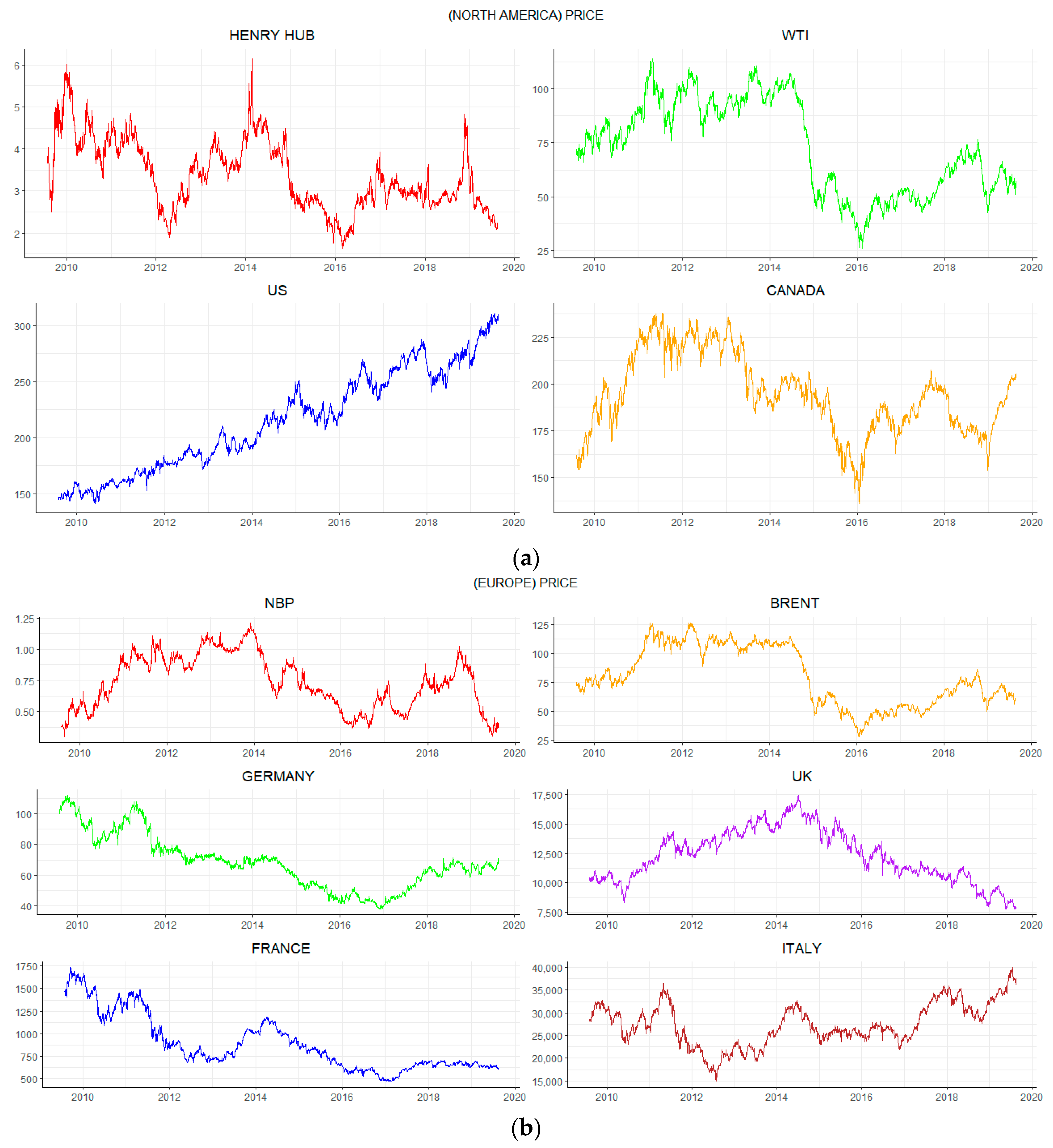
Figure 1a shows images of the prices of natural gas, crude oil, and the electricity utility sector indices in North America. Figure 1b illustrates the natural gas, crude oil, and electricity utility sector indices in Europe. As we can see, in the North America market, the price of the natural gas, crude oil, and electricity utility sector index in Canada follow similar trends and fluctuate violently. These trends dropped dramatically from 2014 to 2016 due to the international oil price crisis. In general, the electricity utility sector index in the US increased continuously from 2009 to 2019, after the global financial crisis of 2007–2009. Relatively, in the European market, Figure 1b shows that the prices of natural gas, crude oil, and the electricity utility sector index follow a semblable non-stationary trend. Moreover, due to international oil price crisis of 2014–2016, energy prices dropped to varying degrees during this time period.
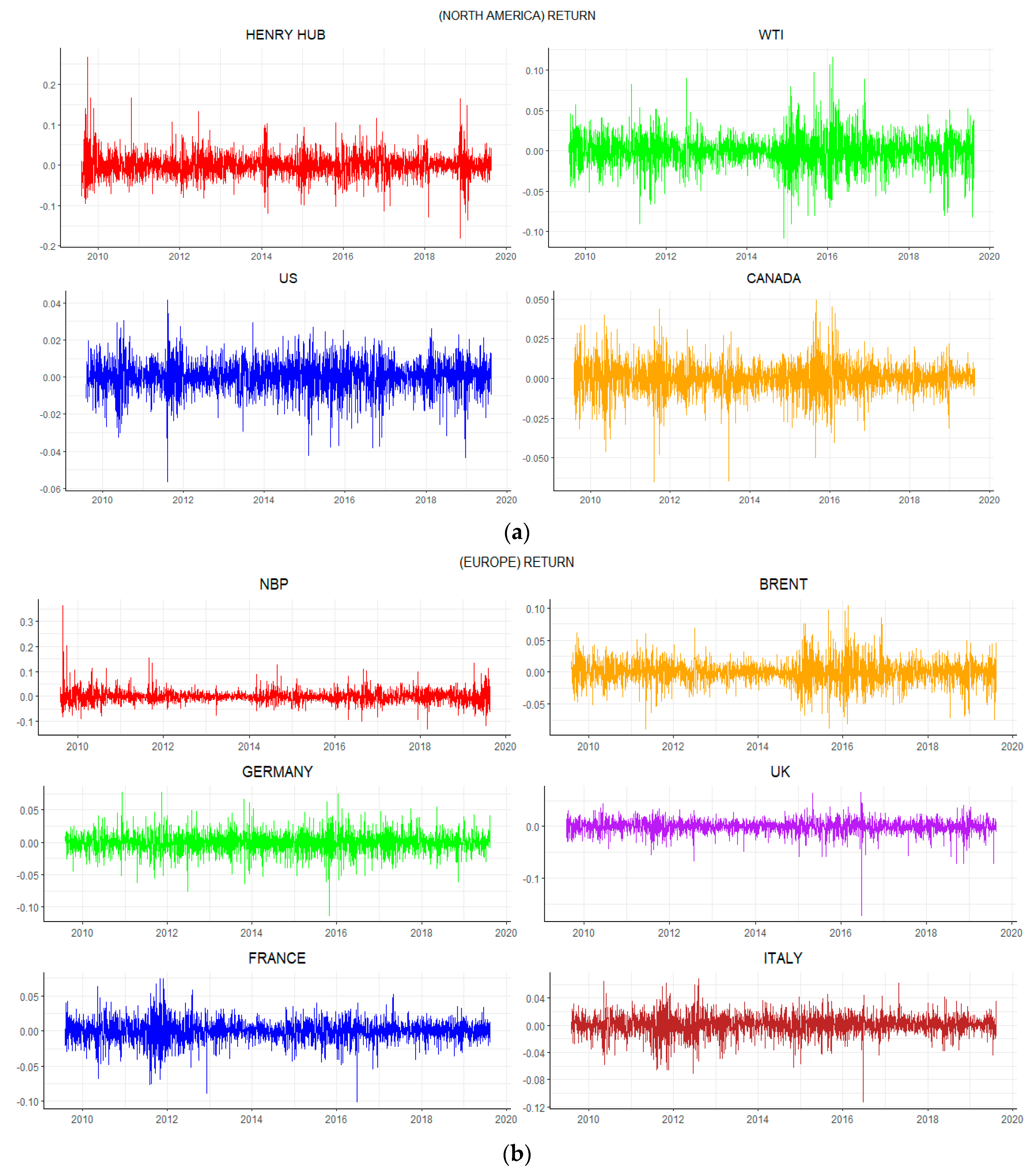
In our analysis, we calculated the closing price of the North American market and the European logarithmic difference as the daily return data, as shown in 
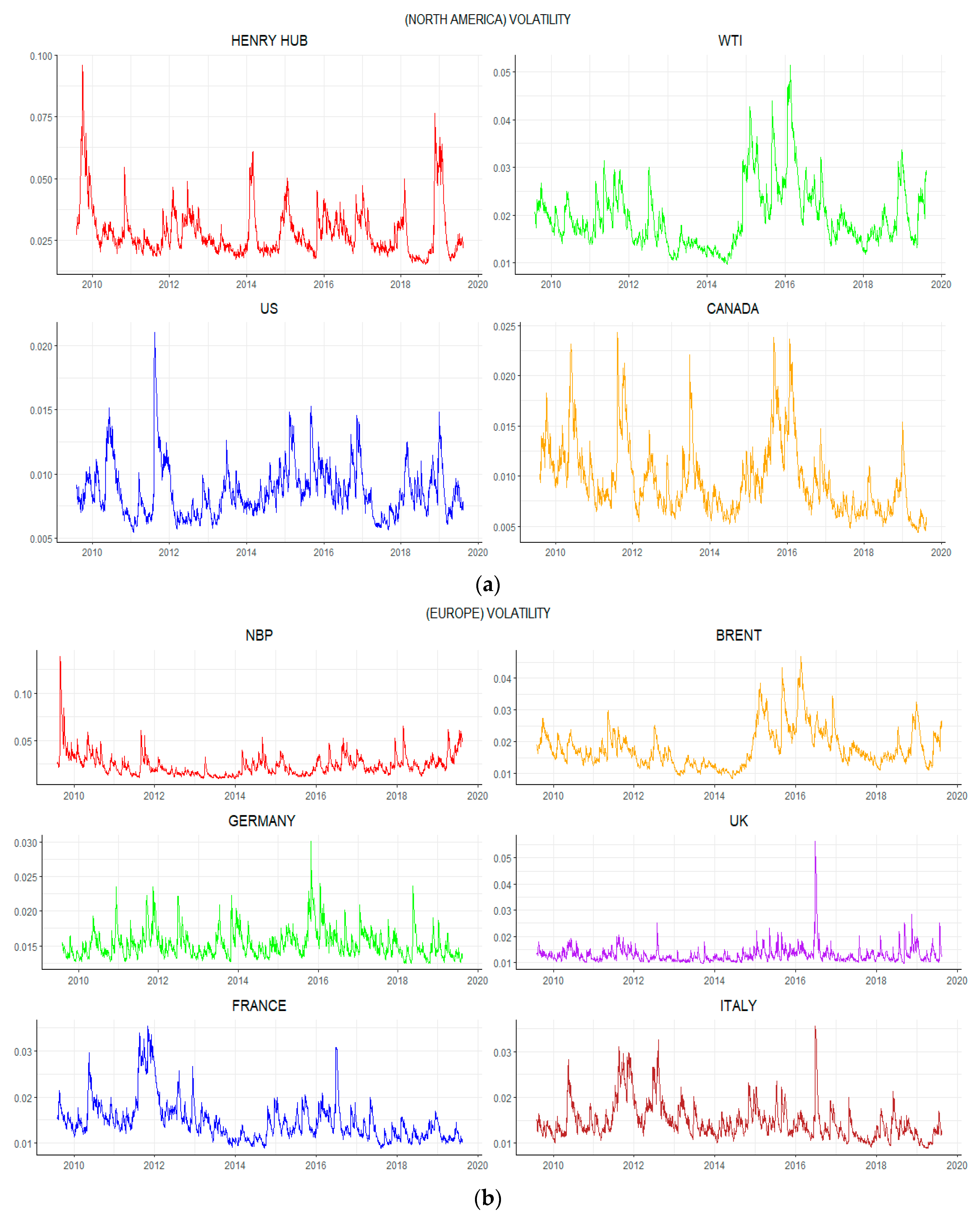
Figure 2a,b. Furthermore, we use the Ljung-Box, which has a lag of 20 to test the time variations of the return series and confirm that the return of all variables is not a white noise series with 10% significance. We use the ARMA (Autoregressive Moving Average)–GARCH model to calculate the volatilities of four assets in North America and six assets in Europe, and the plots are shown in Figure 3a,b. Additionally, the lag of the GARCH model is determined on the basis of the Akaike Information Criterion (AIC).
The descriptive basic statistics of the return and volatility series are shown in Table 2, Table 3. In North America, we find that the mean returns of natural gas and crude oil have negative values. However, the others have positive mean returns. Furthermore, natural gas has the largest maximum daily return and the largest minimum daily return. Specifically, we find that natural gas is the most volatile, followed by crude oil, TSX (Canada), and the S&P 500 (US). Moreover, based on skewness, we find that, except for natural gas, the returns are left-skewed, whereas the return of natural gas is right-skewed. Meanwhile, according to kurtosis, the volatility of the four assets are right-skewed. Regarding kurtosis, the returns and volatilities of the four assets are leptokurtic, which means that the four variables will show more peaked and fat tails. Finally, as the most commonly used unit root testing method, the augmented Dickey–Fuller (ADF), proposed in 1981, tests the null hypothesis that a variable has a unit root, which means that the variable is nonstationary. From the ADF results, the null hypothesis is rejected at 1% significance level for all variables.
Meanwhile, in the European market, in contrast to the North America market, we see that the mean returns of crude oil, DAX (Germany), FTSE 350 (UK), and CAC (France) have negative values. However, the others have positive mean returns. Natural gas has the largest maximum daily return, and FTSE 350 (the UK) has the largest minimum daily return. However, we find that natural gas is the most volatile, followed by crude oil, DAX (Germany), CAC (France), FTSE Italia (Italy), FTSE 350 (UK), and DAX (Germany). On the basis of skewness, the returns of natural gas and crude oil are right-skewed, but the others are left-skewed. In addition, the volatilities of the six assets are right-skewed. Regarding kurtosis, except for the return of CAC (France), which is platykurtic, the returns of the others are leptokurtic. Moreover, the volatilities of the six assets are leptokurtic. Eventually, based on the ADF results, we reject the null hypothesis of a unit root at 1% significance level for all series.

5. Empirical Results

5.1. Spillover Results

We followed Diebold and Yilmaz [1] (hence, DY12) to obtain the spillover effects in the time domain. We first estimated the four variables in our VAR model in the North American market and the six variables in our VAR model in the European market. Then, we used the generalized variance decomposition for a forecast error to set up the spillover table to measure the direction and intensity of spillover across the selected markets.
Next, in frequency domain, following Barunik and Krehlik [2] (hence, BK18), we used Fourier transform to decompose the spillover table in the DY12 model into three different frequency bands, stated in Toyoshima and Hamori [20] as the short-term, “Fre S,” roughly corresponding to 1 to 5 days; the medium-term, “Fre M,” roughly corresponding to 6 to 21 days; and the long-term, “Fre L,” roughly corresponding to 22 days to infinity.
In this study, the lag length of the VAR model is based on the AIC. According to our BK18 model, if the forecasting horizon is (H) < 100, the method is invalid. Consequently, we used a 100-day ahead forecasting horizon (H) for variance decomposition.
In Table 4, Table 5, we show the return spillover results from DY12 and BK18, which include the two markets: North America and Europe. Specifically, Table 4 and Table 5 includes four sub-tables. At the top are the results of the DY12, followed by the short-term, the medium-term, and the long-term results from the BK18. In each sub-table, the values in the ith row and the jth column equate to the strength of the spillover effect from the jth market to the ith market. For example, in the DY12 return spillover results in the North American market, the strength of the spillover effect in the third column (US) and the second row (WTI) is 2.264. The values in the last row called “TO” indicate the mean value of the spillover effect on the other markets, whereas the values in the last column called “FROM” indicate the mean value of the spillover effect from the other markets. The total spillover is the summary of all “TO” or “FROM” (for example, 17.165, as shown in the lower right corner).
Next, we identify some specifics when we compare the difference between the return spillover effect in North America and in Europe using the pure time-domain approach of DY12. First, for the total return spillover effect, we can see that the total return spillover effect in Europe (30.245%) is stronger than that in North America (17.165%). This demonstrates that the return connectedness of natural gas, crude oil, and the electricity utility sector index in Europe is stronger than that in North America. Whether in North America or Europe, the total return spillover of crude oil contributes more than natural gas to the electricity utility stock market in each country. Further, in North America, Canada receives a greater effect from the two energy futures (0.318% from natural gas and 11.8% from crude oil) compared with the US in the time domain. In contrast, Canada exerts a greater effect on the natural gas (0.394%) and crude oil (13.697%) sectors in the time domain. In Europe, the UK receives the greatest effect from the two energy futures (0.757% from natural gas and 3.889% from crude oil) compared with the other three countries in the time domain. The UK transmits the greatest effect on natural gas (1.249%), but France transmits the greatest effect on crude oil (6.353%) in the time domain, which contrasts with the situation in North America. Finally, we find that there are some differences in the return spillover effect among the two commodity markets and the stock market in North America and Europe, respectively. In North America, we find that the US receives a greater return spillover effect on natural gas (0.163%) and transmits less of an effect (0.147%). In contrast to the US, Canada transmits more of a return spillover effect on natural gas (0.394%) and receives a smaller effect (0.318%). In contrast to the natural gas market, the US transmits more of a return spillover effect on crude oil (2.264%) and receives a smaller effect (2.242%). In the same vein as the US, Canada also transmits more of a return spillover effect on crude oil (13.697%) and receives a smaller effect (11.8%).
In Europe, except for Germany, the other three stock markets transmit more of a return spillover effect on natural gas and receive a smaller effect. In the same vein as the situation for natural gas, except for Germany, the other three stock markets transmit more of a return spillover effect on crude oil and receive a smaller effect. In terms of frequency, Table 4 and Table 5 reveal that looking at either North America or Europe, the total return spillover in the short-term (Frequency S 1–5 Days) is the highest, followed by the medium-term (Frequency M 6–21 Days) and the long-term (Frequency L 22–Infinity Days). These results suggest that the return shocks from any market transmitted to another market will not exceed one week.
Table 6, Table 7 show the volatility spillover results of DY12 and BK18 with the same construction. Table 6 shows the volatility spillover effect in North America, and Table 7 shows the effect in Europe. In time domain of DY12, we find the following. The total volatility spillover effect in Europe (27.929%) is stronger than that in in North America (20.216%). This situation is the same for the total return spillover; whether in North America or Europe, the total volatility spillover of crude oil transmits more than natural gas to the electricity utility stock market in each country. In North America, between the two stock markets, Canada receives the greatest spillover effect from natural gas (0.664%), and the US receives the greatest effect from crude oil (6.771%) in the time domain. Among the two commodity markets, WTI is the most influential market on the stock market, transmitting the largest volatility spillover to the US (6.771%) and Canada (6.302%) and is also the market that receives the largest volatility spillover from the US (4.373%) and Canada (19.036%) compared with the natural gas market.
In the European market, among the four stock markets, the UK receives the largest effect from natural gas (0.785%), and Germany receives the largest effect from crude oil (4.56%) in the time domain. However, the UK transmits the largest effect on crude oil (8.843%), and Germany transmits the largest effect on natural gas (2.374%) compared with other countries in the time domain. In addition, in terms of frequency and in contrast to the return spillover, Table 6 and Table 7 reveal that in both North America and Europe, the total volatility spillover for the long-term (Frequency L 22–Infinity Days) is the highest, followed by the medium-term (Frequency M 6–21 Days) and the short-term (Frequency S 1–5 Days). These results imply that volatility shocks have a long-lasting effect.

5.2. Dynamic (Moving-Window) Analysis

We have useful results on the total spillover effects from our full sample. However, these results are not helpful in analyzing how connectedness changes over time. If we only focus on the static results, the VAR estimated over the whole sample may smooth out the results when there is time variation in the relationship between the variables (Lovcha [21]). In order to better understand the dynamics of spillover effects, we employ a moving-window to analyze the spillover results of DY12 and BK18. For the moving-window method, we keep the forecast horizon at 100, which is used in the static analysis. For example, Toyoshima and Hamori [20] employ 100–day rolling samples. Jorion [32] sets a 20–day window for estimation. Blanchard et al. [33] used a five–year rolling standard deviation of output growth in the US. Similarly, we set the length of the window at 250 trading days, 370 trading days, and 500 trading days, and find that the plots of these trading days have almost the same trends. We put the results into Appendix A. For this reason, we chose 500 trading days for the length of the moving-window to keep the rolling sample large enough to ensure the stationarity of the series in each VAR estimation.
As displayed in Figure 4a,b, we find some characteristics from the dynamics of the total return spillover and the frequency decomposition of North America and Europe. In both North America and Europe, the total return spillover occurs in the short-term. Moreover, two dynamic return spillover figures have a similar trend. In Europe, the total spillover of the DY12 model for the return series varies between 20% and 45%, which is wider than that in North America (between 10% and 30%). From 2009 to mid–2013, whether in North America or Europe, the total return spillover retains high stability, which may be a consequence of the effect of the 2008 global financial crisis or the 2010 European sovereign debt crisis. The total return spillover in both North America and Europe began to increase steadily until around 2017, which could be influenced by the 2014 international crude oil crisis.
As seen in Figure 5a,b, which shows the dynamics of total volatility spillover and frequency decomposition for North America and Europe, the total spillover fluctuates more than the total return spillover. Moreover, the total volatility spillover reacts more violently to extreme events than that of the returns. In contrast with the total return spillover, the total volatility spillover develops over the long-term. This means that the total volatility spillover is more sensitive to shocks and extreme events; unlike the total return spillover, whether in North America or Europe, the total volatility spillover of DY12 shifts between 0% and 60%. From 2009 to mid-2013, whether in North America or Europe, the total volatility spillover retained its stability, which may be a consequence of the 2008 global financial crisis and the 2009 European sovereign debt crisis. In North America, we identified some sudden fluctuations, such as a sharp increase in 2015 and 2016, an increasing trend from 2017 to 2018, and a sudden rise in 2019. These fluctuations may have been influenced by the 2014 international crude oil crisis, the 2016 Organization of the Petroleum Exporting Countries announcement to cut supplies at the end of 2017, the 2017 summer Hurricane Irma, and the 2019 trade war between China and the US. However, in Europe, we see almost the same fluctuations from mid-2013 to 2016; around 2015 to mid-2016, there are two sudden fluctuations that may be a result of some extreme events, such as the 2014 international crude oil crisis and the 2016 Brexit event. We also investigated the dynamics of the total return and volatility spillover in different windows and the pairwise directional return and volatility spillover in two regions. The results are given in Appendix A.

6. Concluding Remarks

Our paper discusses the return and volatility spillover across the natural gas market, crude oil market, and stock market from 4 August 2009 to 16 August 2019 to assess the information transmission and risk transmission among the three markets by employing a new method for time–frequency developed by Diebold and Yilmaz [1] and Barunik and Krehlik [2]. It is crucial to investigate the spillover effects not only for investors to adjust their investment programs but also for government authorities to make proper economic decisions. The contributions of our paper to the literature are as follows.
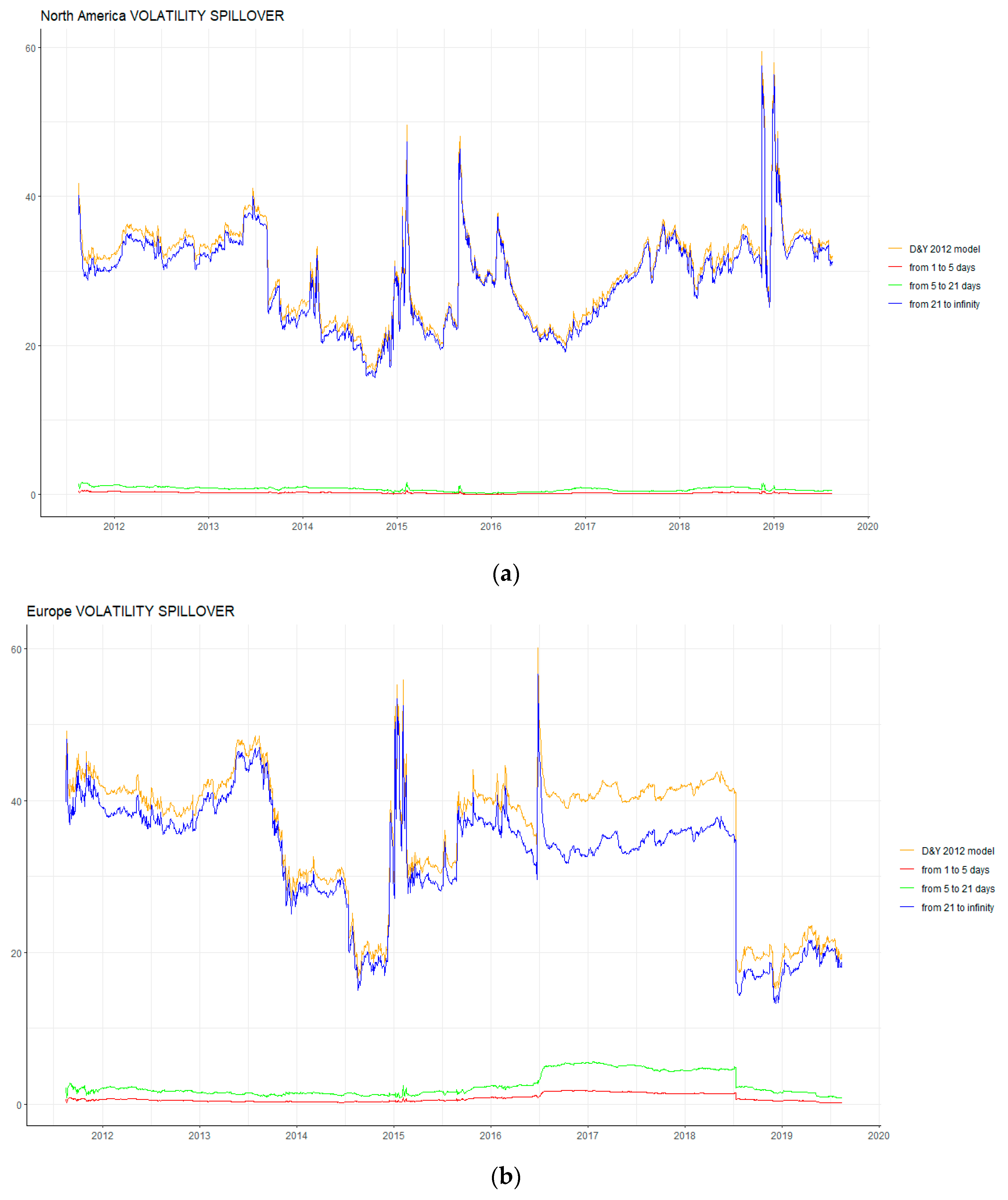
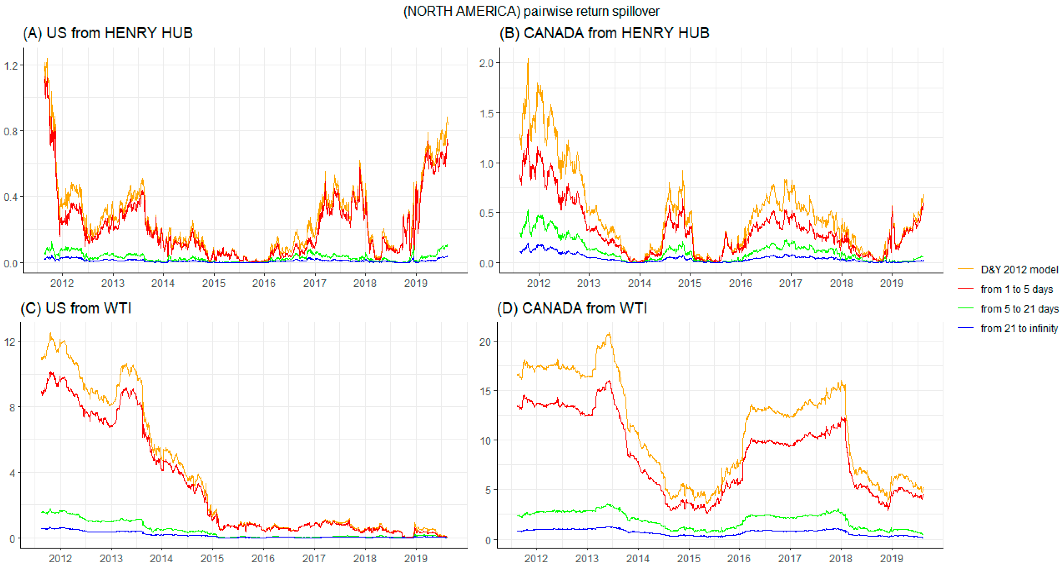
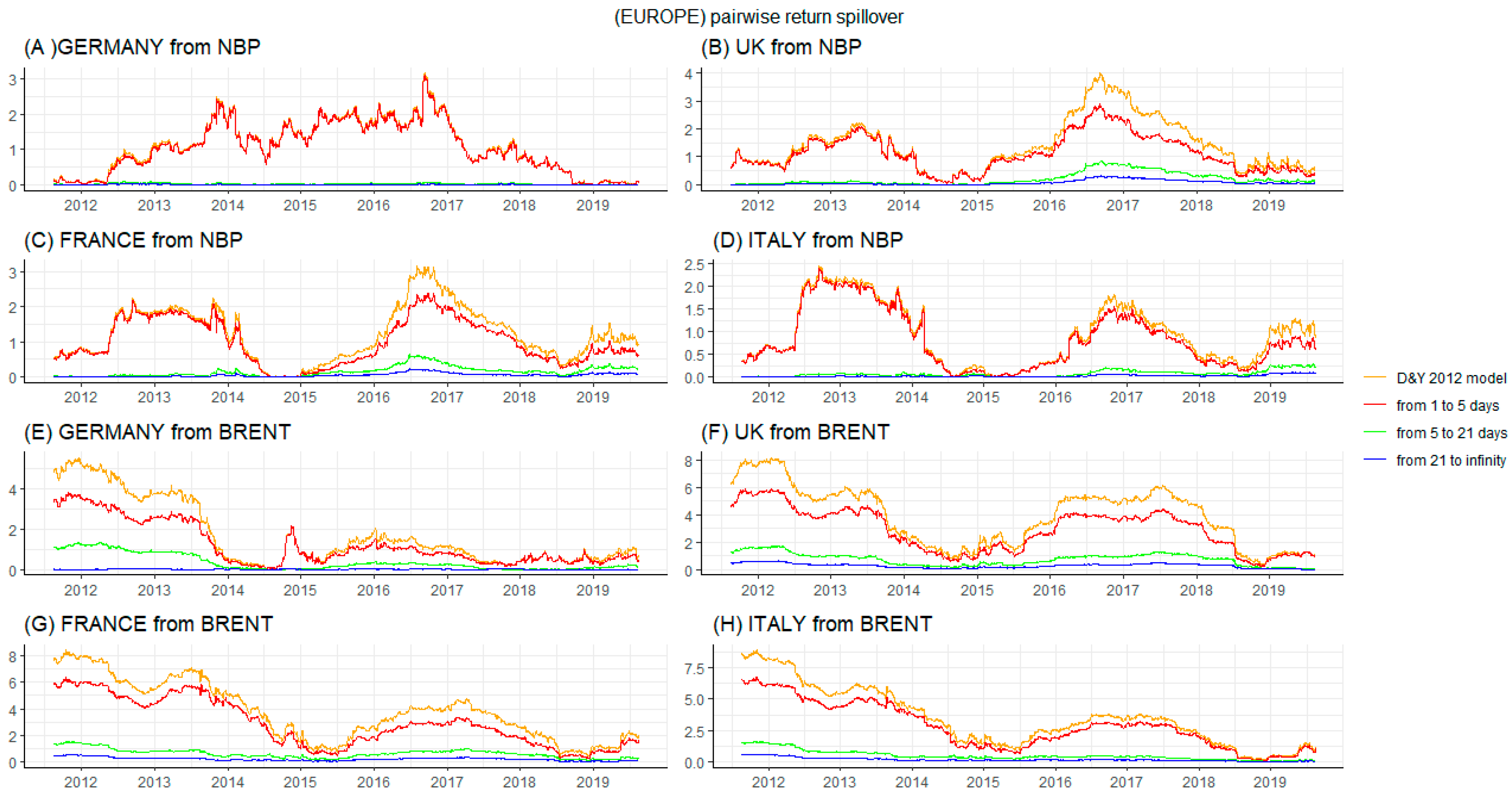
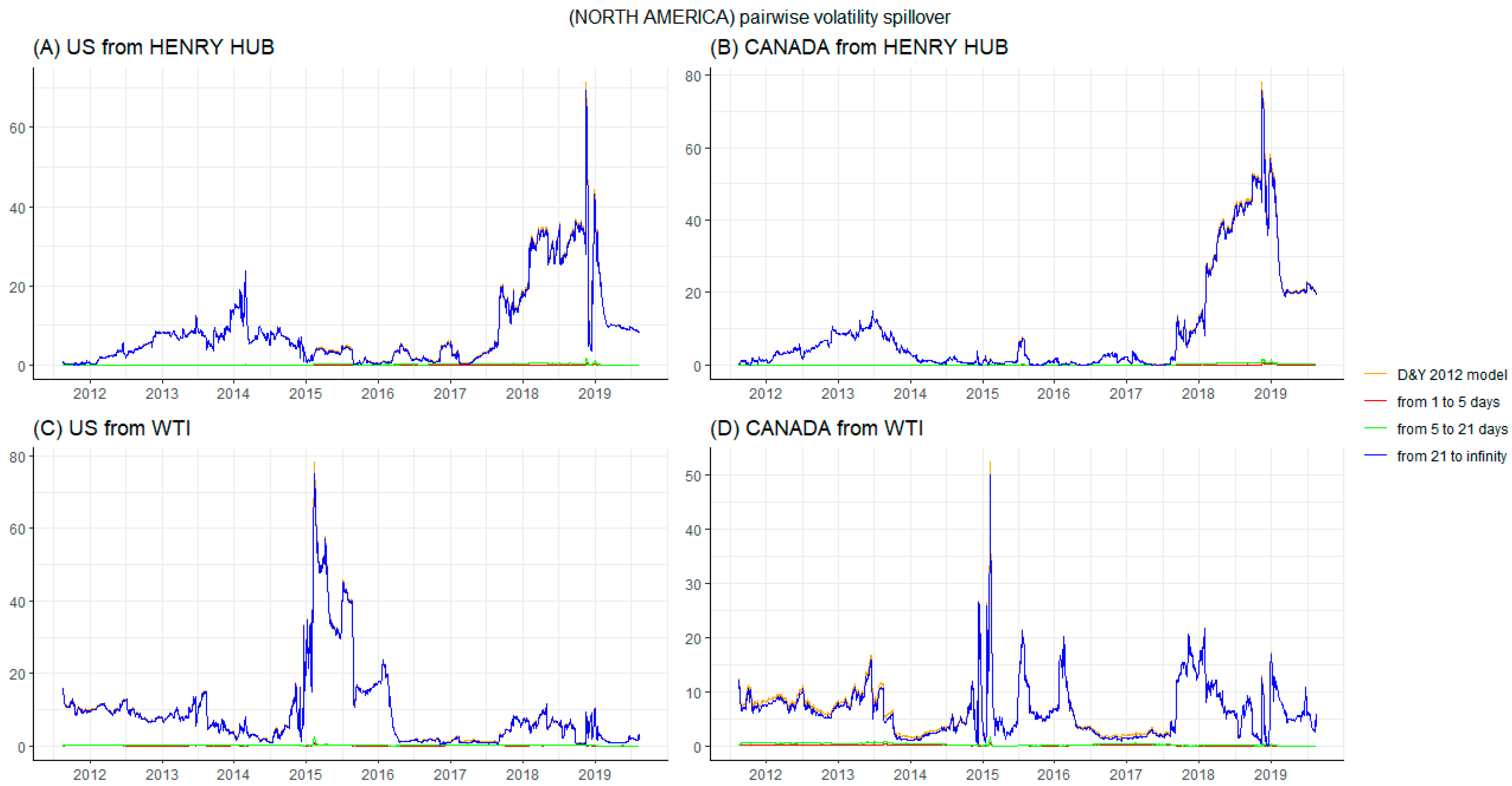
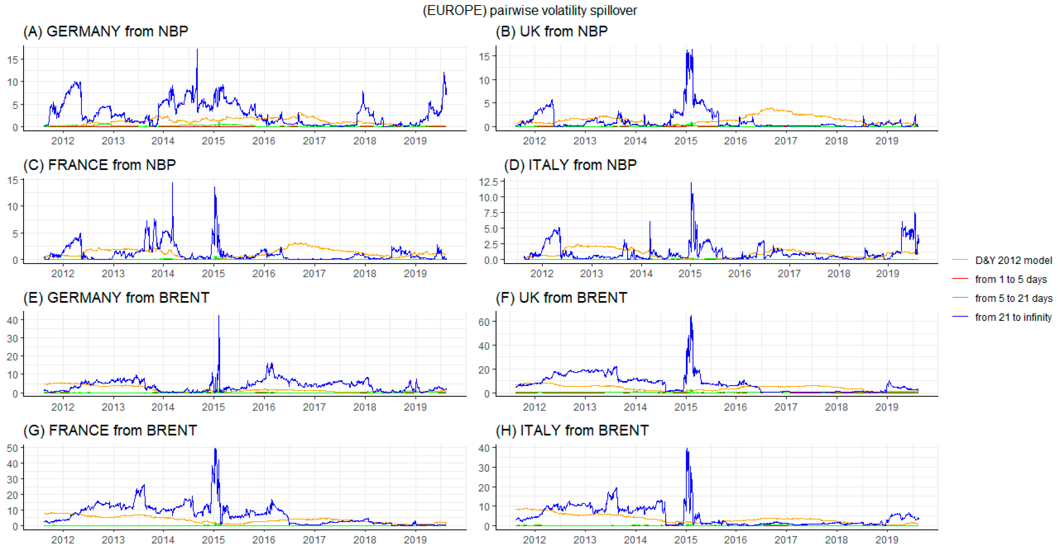
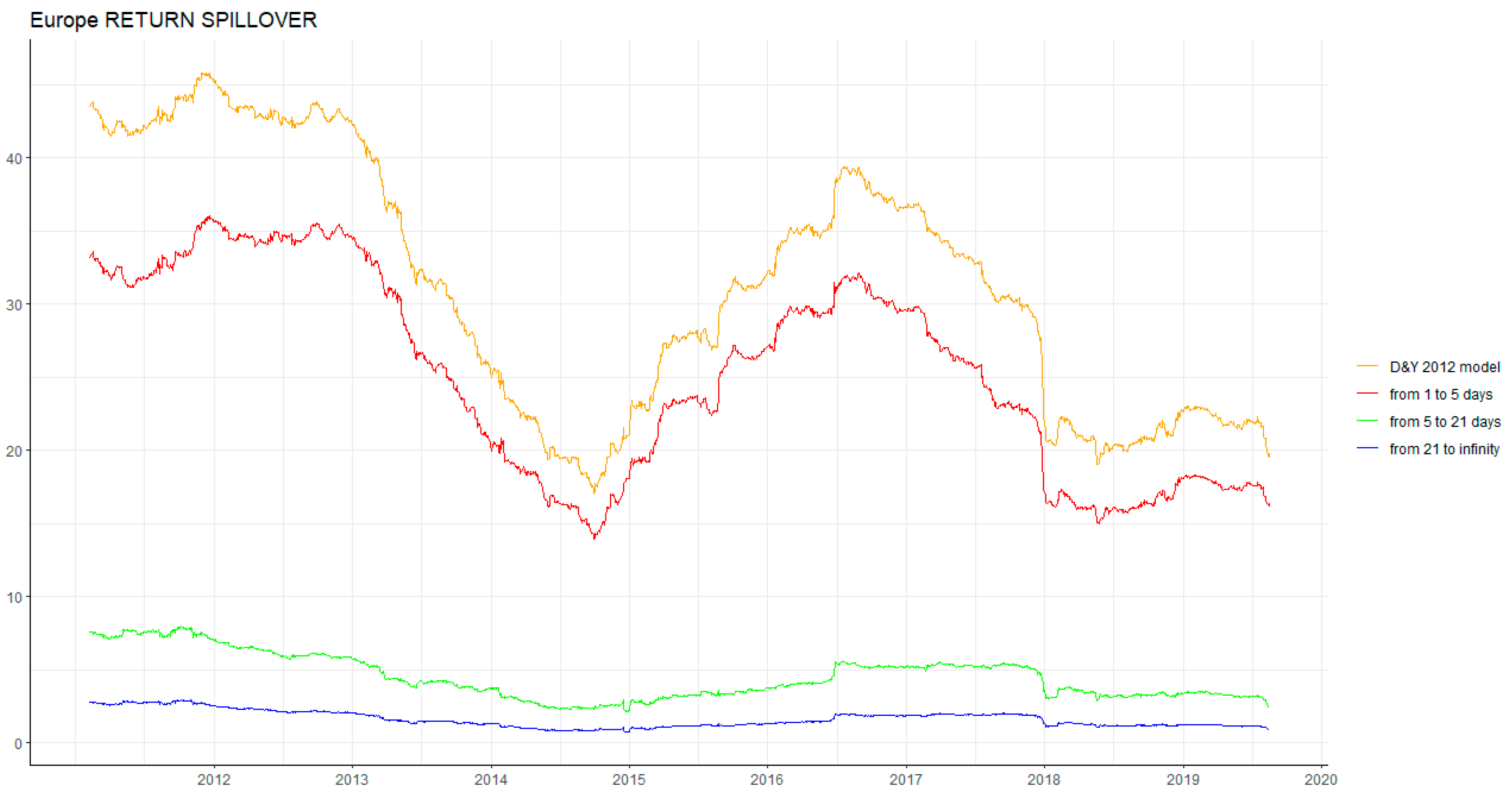
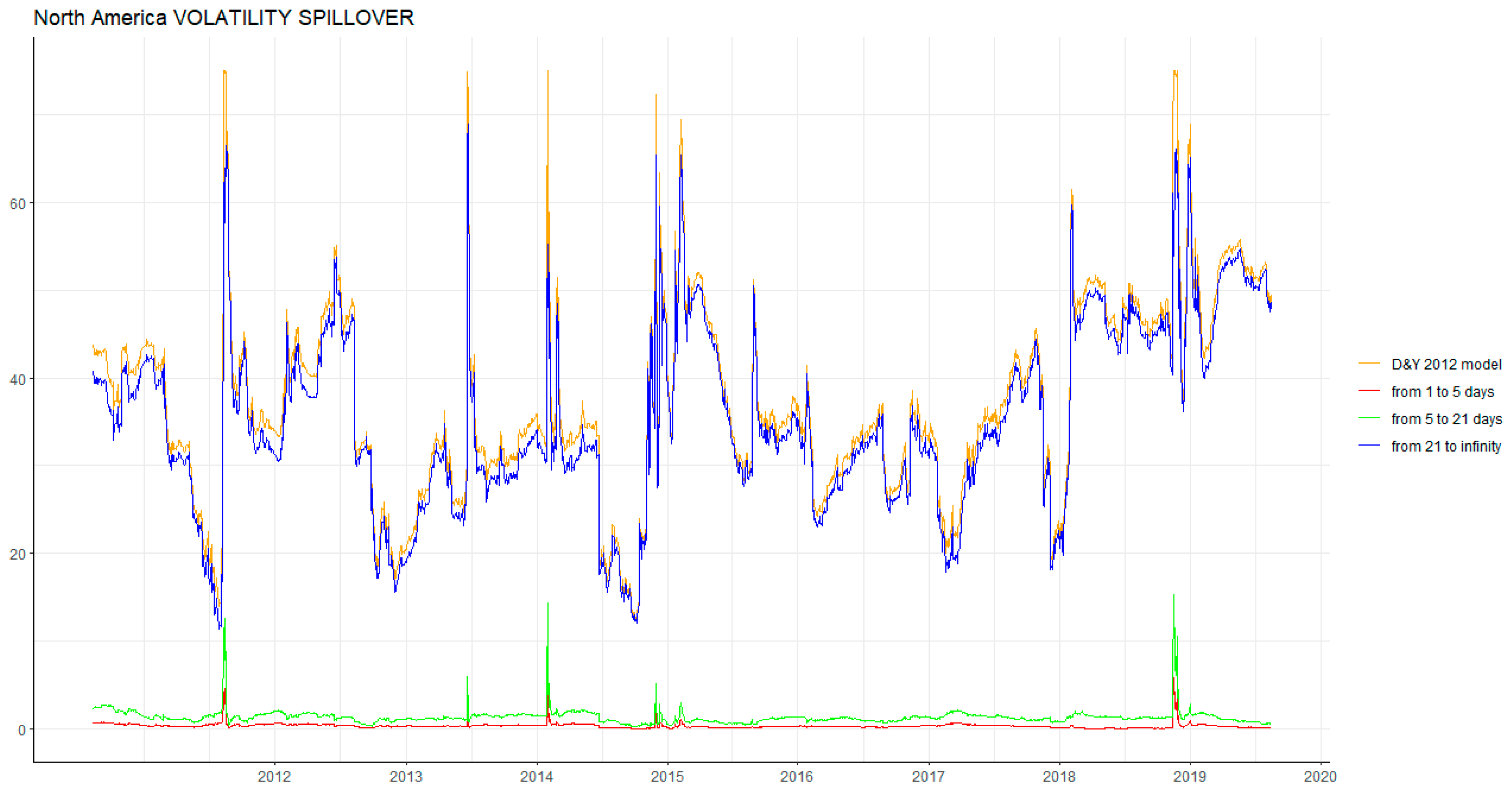
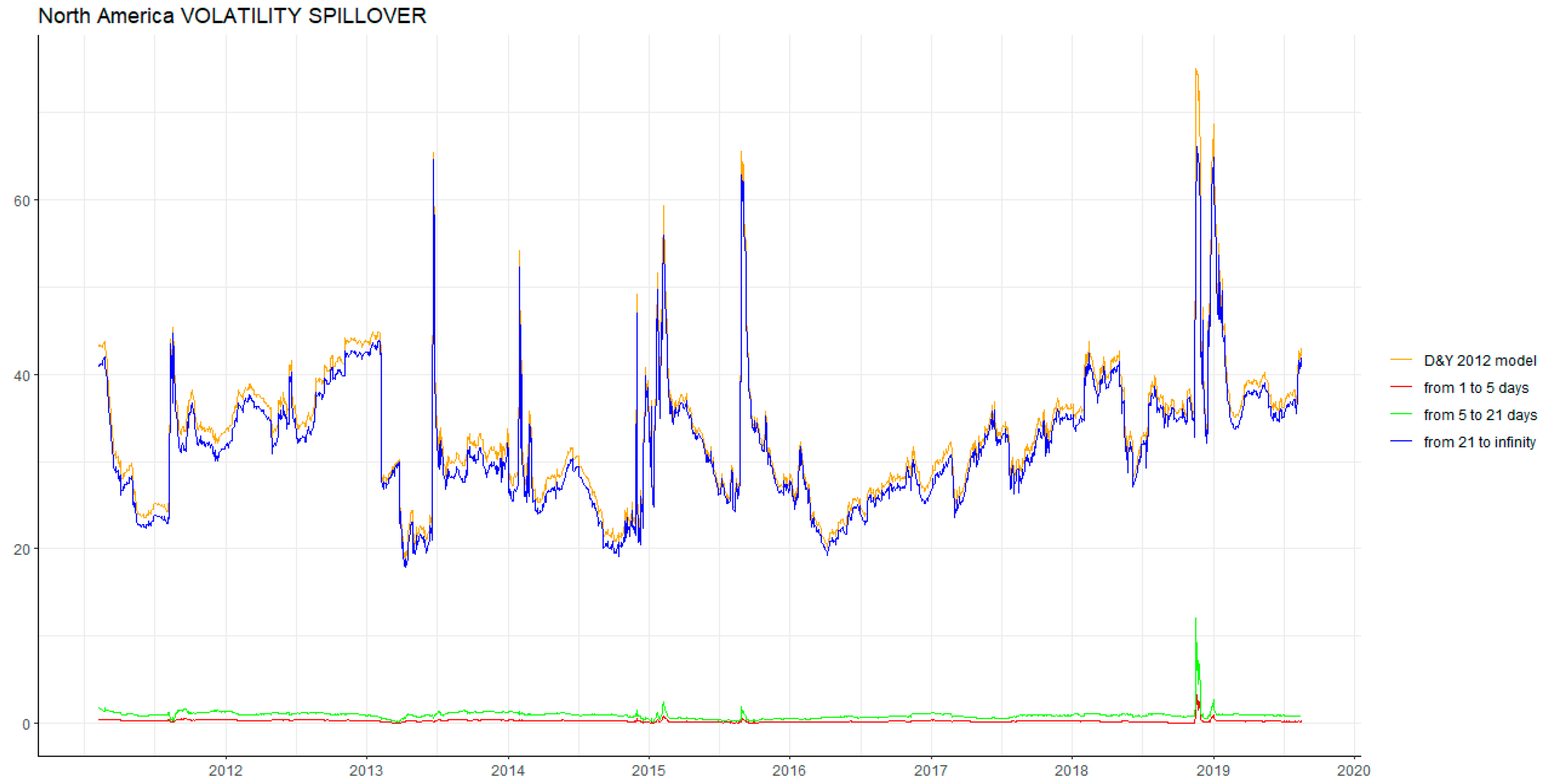
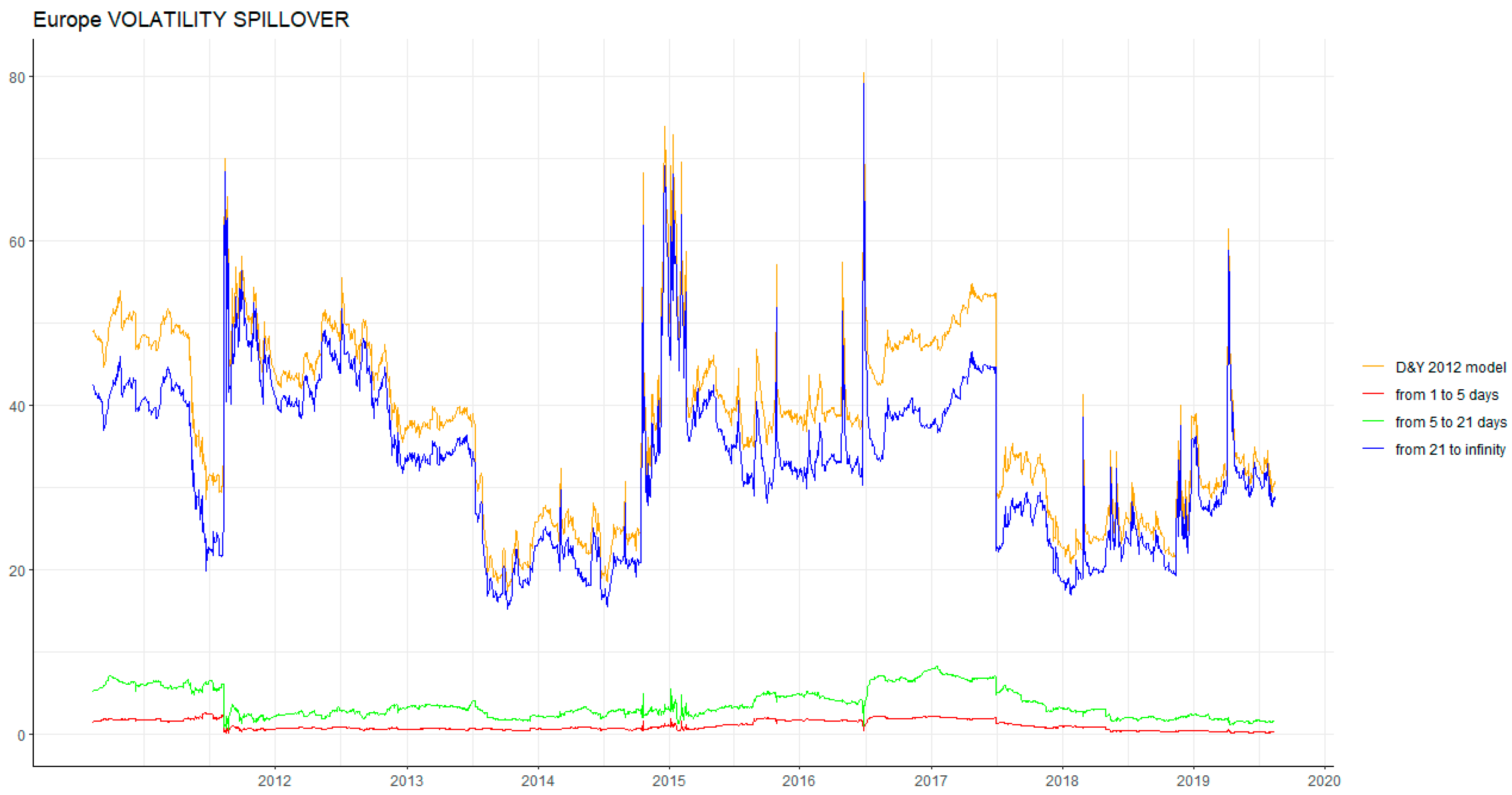
First, in time domain, the total return and volatility spillover in Europe are stronger than in North America. Moreover, whether in North America or in Europe, the spillover table reveals that crude oil, rather than natural gas, has the greatest effect on electricity utility stock markets. In North America, Canada not only receives a larger return spillover effect from the two energy futures (0.318% from natural gas, 11.8% from crude oil) compared with the US but also transmits a greater effect on the two energy futures. Regarding volatility spillover, Canada still has the largest spillover effect on the other two energy futures and receives the largest volatility effect from natural gas. However, the US receives the largest volatility spillover effect from crude oil (6.771%). In Europe, the UK receives the greatest return spillover effect from the two energy futures (0.757% from natural gas and 3.889% from crude oil) compared with the other three countries. The UK transmits the largest effect on natural gas (1.249%), but France transmits the largest effect on crude oil (6.353%) in the time domain, which is different than the situation in North America. Regarding volatility spillover, the UK receives the largest effect from natural gas (0.785%), and Germany receives the largest from crude oil (4.56%). However, FTSE350 (the UK) transmits the largest effect on crude oil (8.843%), and Germany transmits the largest effect on natural gas (2.374%) compared to the other countries.
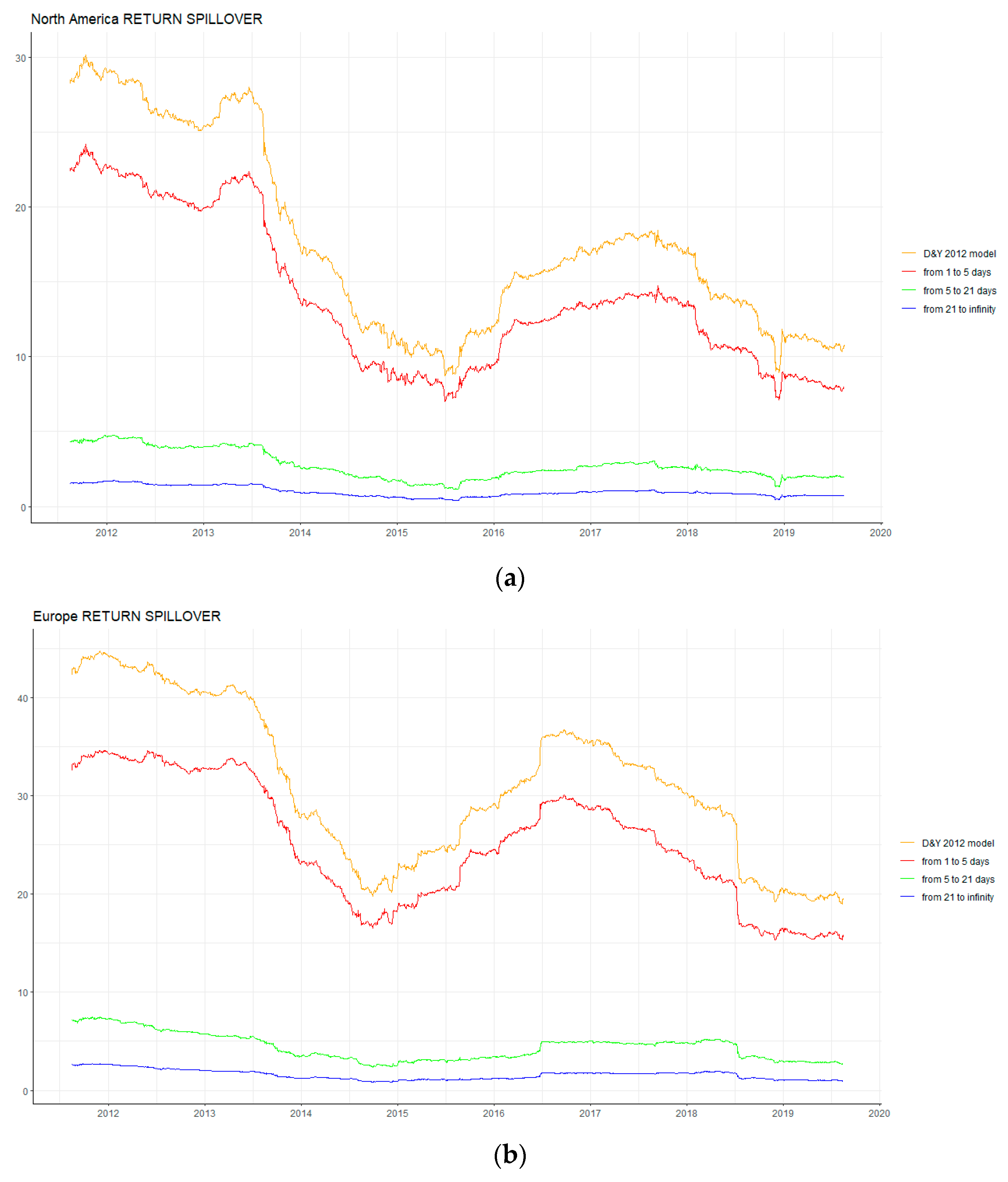
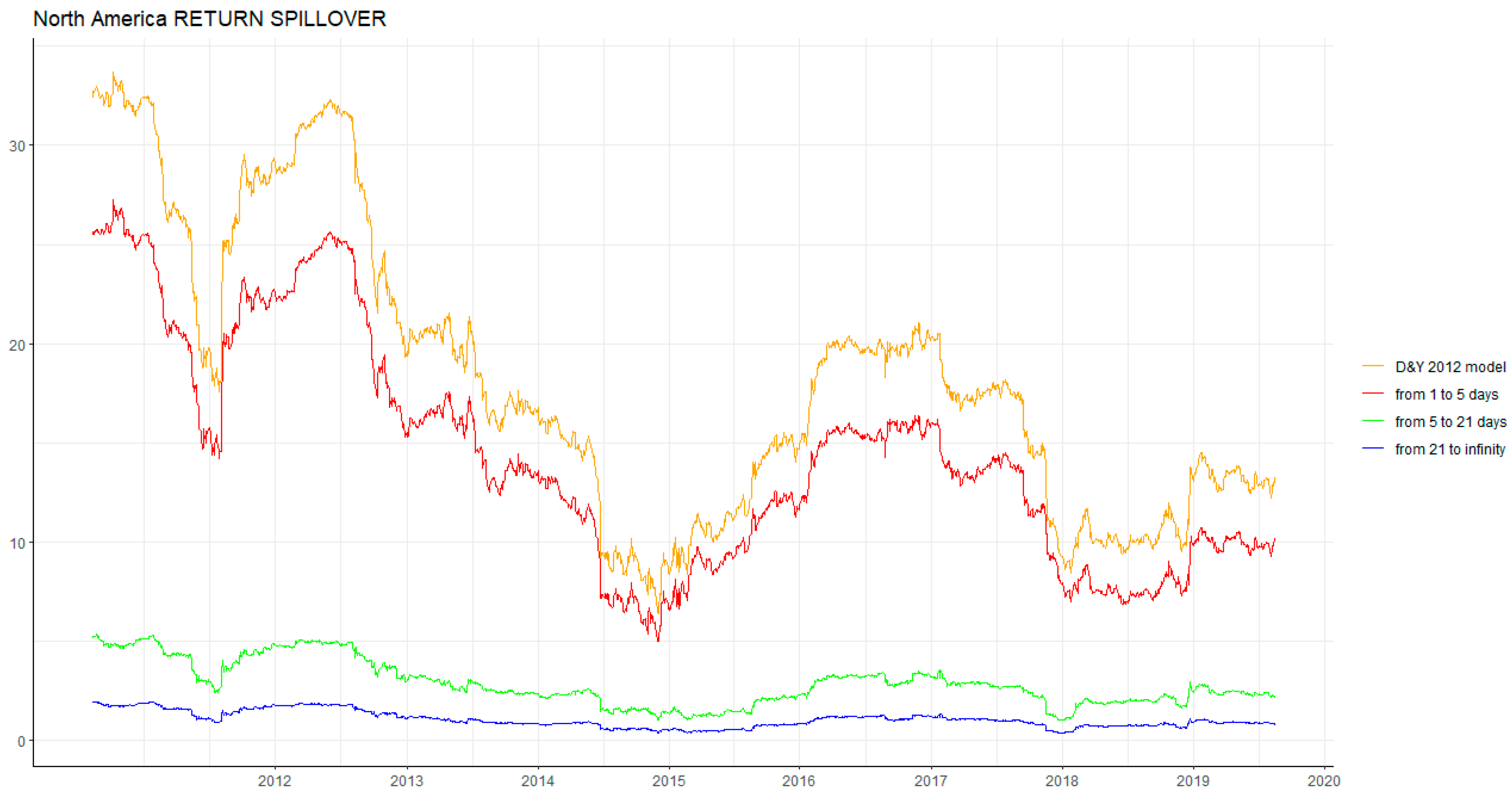
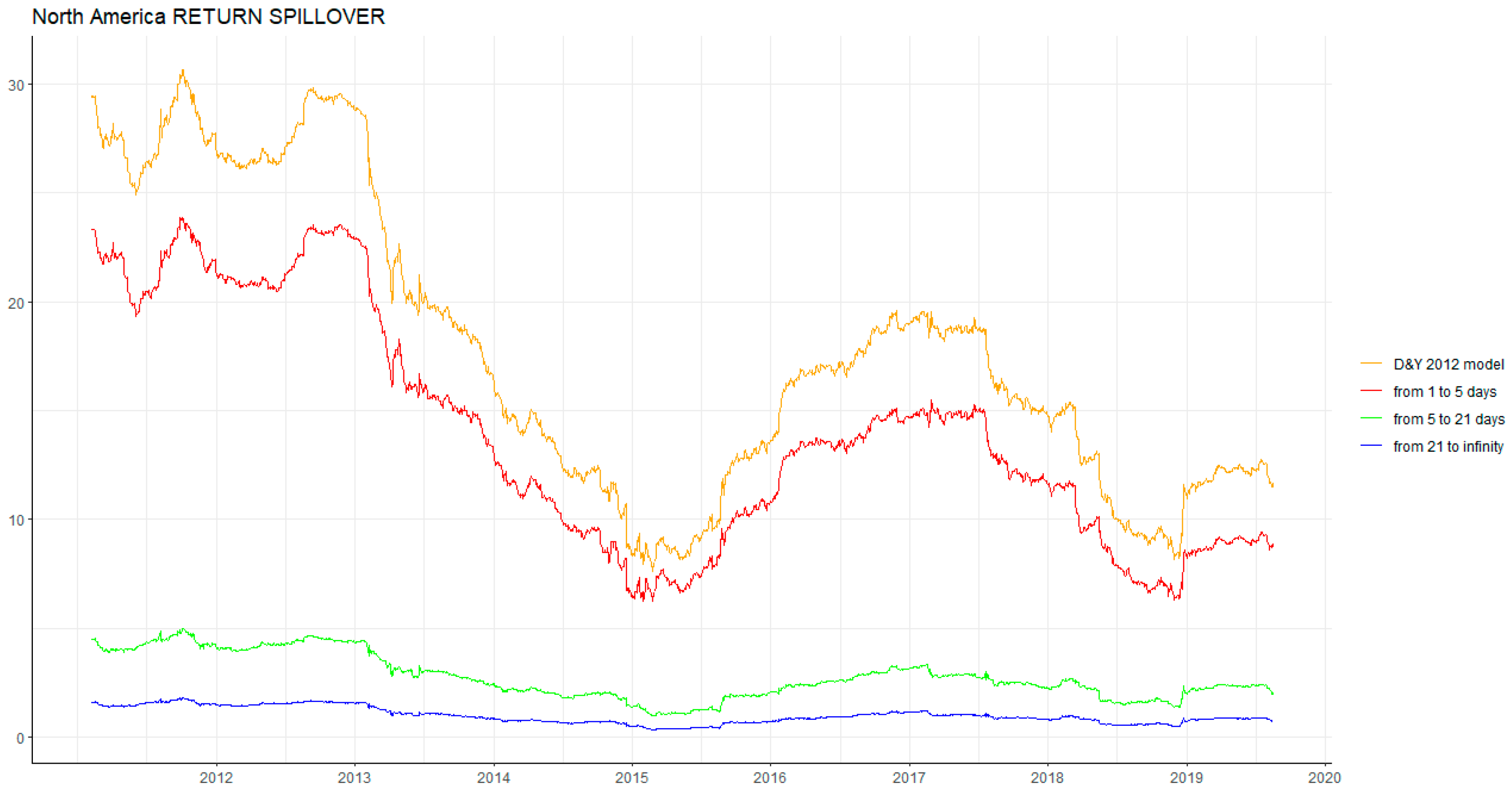
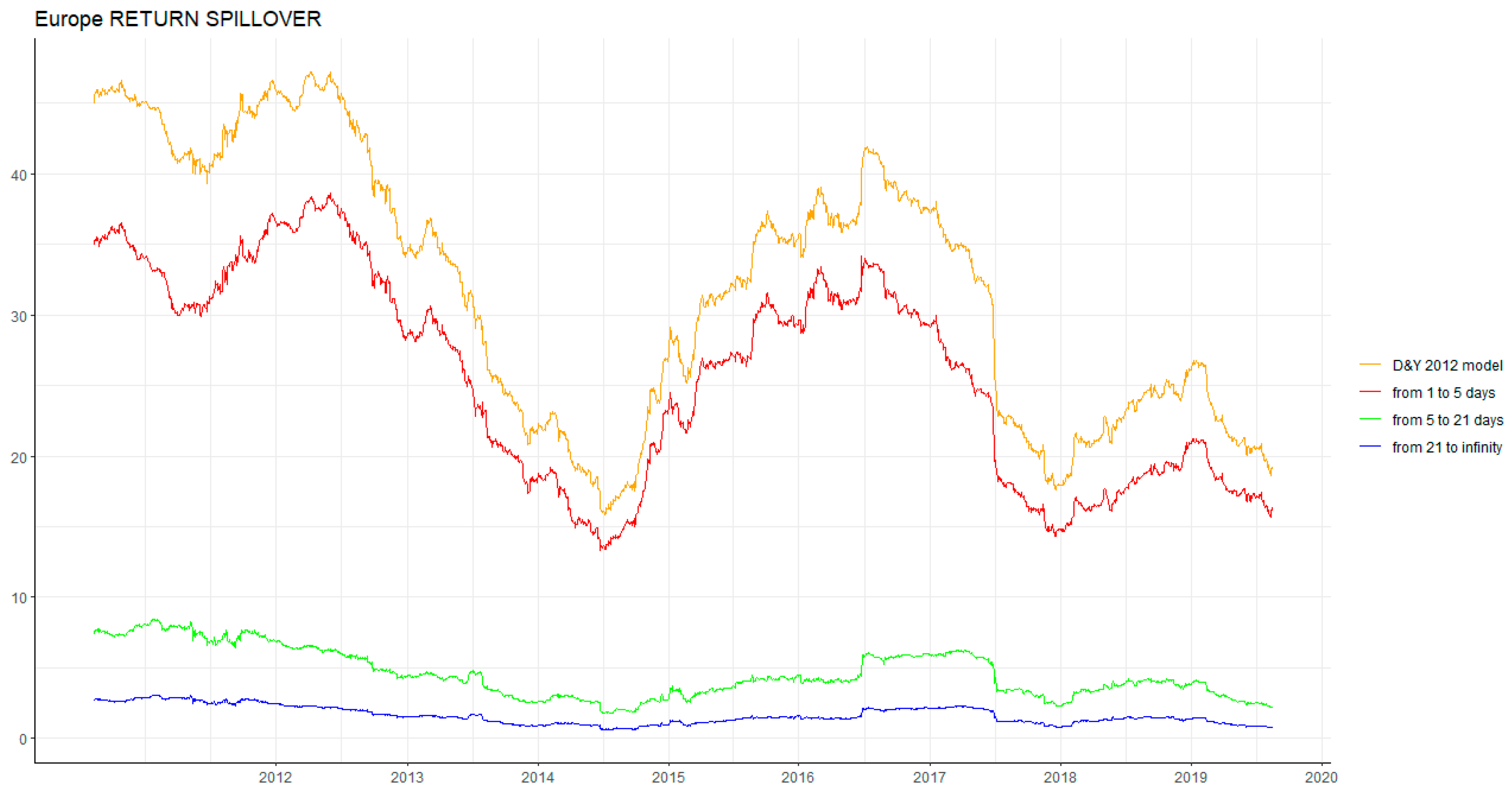
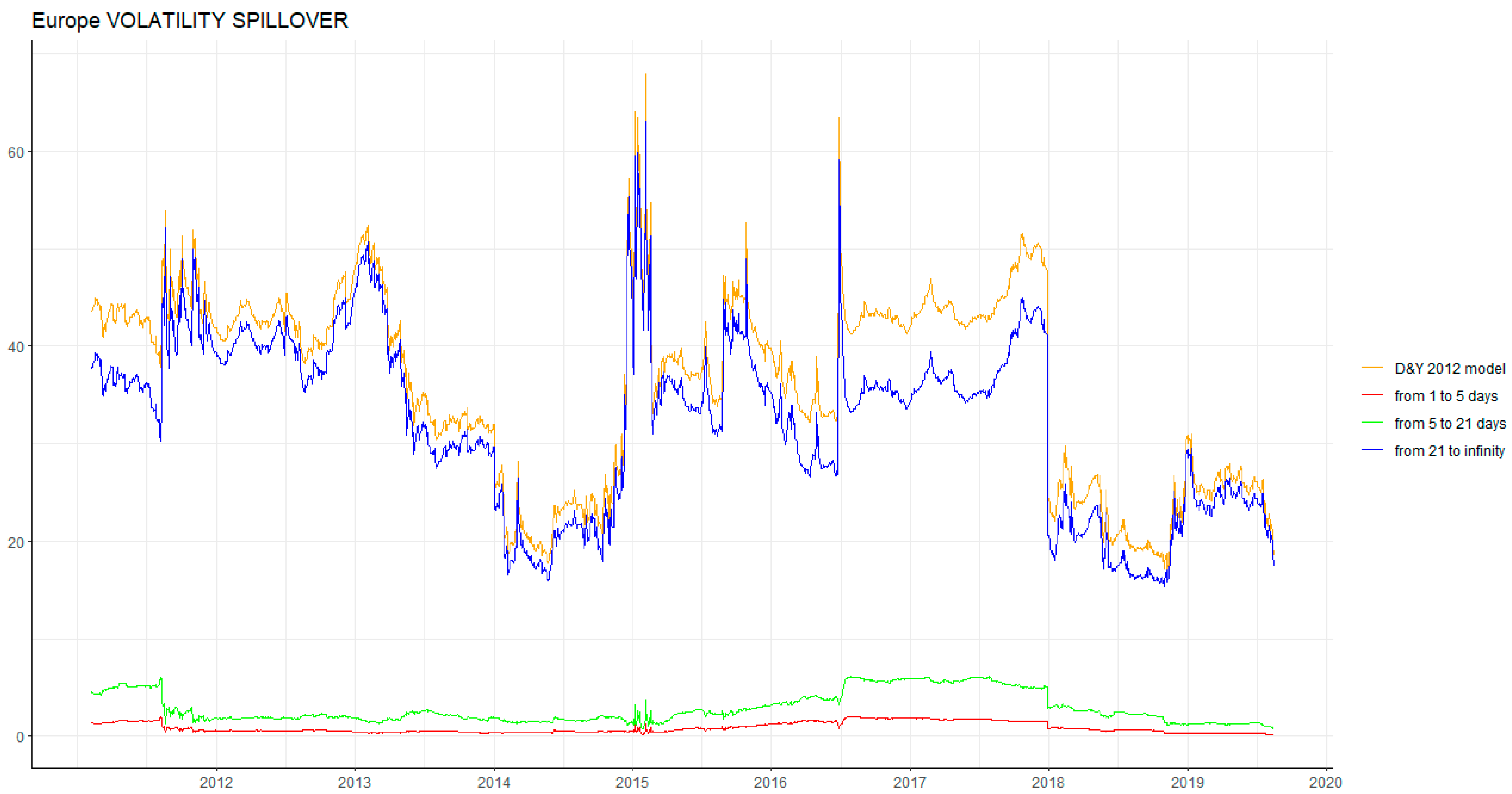
Second, in terms of frequency, our results show that the short-term has the largest effect on return spillover; however, the long-term has the largest effect on volatility spillover in both North America and Europe. These results imply that the return shocks from any market transmitted to another market will not exceed one week, whereas the results of volatility spillovers imply that volatility shocks have a long-lasting effect. This conclusion is consistent with the results of Barunik and Krehlik [2] and Tiwari et al. [34].
Third, in terms of return spillover transmission, all markets respond to return shocks immediately. The total return spillover effect in the short-term was the greatest. In this case, it is difficult to determine the impact of a particular market on another market. Unlike return spillover transmissions, the total volatility spillover effect in the long-term was the greatest. Policymakers have sufficient time to prevent the impact of extreme volatility shocks on other markets. In addition, based on a summary of the results above, the volatility of natural gas is less than that of oil, which suggests that compared with oil, natural gas investors may have a greater opportunity to make a profit.
Forth, some interesting results are displayed in the rolling analyses. For example, because of the subsequent effect of the 2008 global financial crisis and the 2010 European sovereign debt crisis, the return and volatility spillover in both North America and Europe maintained a high level. Due to the later 2014 international oil crisis, both North America and Europe fluctuated fiercely around 2015. Around mid-2016, the Brexit event made the volatility spillover in Europe increase suddenly.

Author Contributions

Conceptualization, T.N. and S.H.; investigation, W.Z. and X.H.; writing—original draft preparation, W.Z.; writing—review and editing, X.H., T.N., and S.H.; project administration, S.H.; funding acquisition, S.H. All authors have read and agreed to the published version of the manuscript.

Funding

This work was supported by JSPS KAKENHI Grant Number 17H00983.

Acknowledgments

We are grateful to Mehmet H. Bilgin and four anonymous referees for helpful comments and suggestions.

Conflicts of Interest

The authors declare no conflict of interest.

Appendix A

Figure A1. Pairwise directional return spillover of DY12 and BK18 in North America. Notes: US from HENRY HUB indicates the return spillover from natural gas to US; CANADA from HENRY HUB indicates the return spillover from natural gas to Canada; US from WTI indicates the return spillover from crude oil to US; CANADA from WTI indicates the return spillover from crude oil to Canada.
Energies 13 00727 g0a1
Figure A2. Pairwise directional return spillover of DY12 and BK18 in Europe. Notes: GERMANY from NBP indicates the return spillover from natural gas to Germany; UK from NBP indicates the return spillover from natural gas to the UK; FRANCE from NBP indicates the return spillover from natural gas to France; ITALY from NBP indicates the return spillover from natural gas to Italy; GERMANY from BRENT indicates the return spillover from crude oil to Germany; UK from BRENT indicates the return spillover from crude oil to the UK; FRANCE from BRENT indicates the return spillover from crude oil to France; ITALY from BRENT indicates the return spillover from crude oil to Italy.
Energies 13 00727 g0a2
Figure A3. Pairwise directional volatility spillover of DY12 and BK18 in North America. Notes: US from HENRY HUB indicates the volatility spillover from natural gas to US; CANADA from HENRY HUB indicates the volatility spillover from natural gas to Canada; US from WTI indicates the volatility spillover from crude oil to US; CANADA from WTI indicates the volatility spillover from crude oil to Canada.
Energies 13 00727 g0a3
Figure A4. Pairwise directional volatility spillover of DY12 and BK18 in Europe. Notes: GERMANY from NBP indicates the volatility spillover from natural gas to Germany; UK from NBP indicates the volatility spillover from natural gas to the UK; FRANCE from NBP indicates the volatility spillover from natural gas to France; ITALY from NBP indicates the volatility spillover from natural gas to Italy; GERMANY from BRENT indicates the volatility spillover from crude oil to Germany; UK from BRENT indicates the volatility spillover from crude oil to the UK; FRANCE from BRENT indicates the volatility spillover from crude oil to France; ITALY from BRENT indicates the volatility spillover from crude oil to Italy.
Energies 13 00727 g0a4
Figure A5. Total return spillover of DY12 and BK18 in North America (Windows 250).
Energies 13 00727 g0a5
Figure A6. Total return spillover of DY12 and BK18 in North America (Windows 370).
Energies 13 00727 g0a6
Figure A7. Total return spillover of DY12 and BK18 in Europe (Windows 250).
Energies 13 00727 g0a7
Figure A8. Total return spillover of DY12 and BK18 in Europe (Windows 370).
Energies 13 00727 g0a8
Figure A9. Total volatility spillover of DY12 and BK18 in North America (Windows 250).
Energies 13 00727 g0a9
Figure A10. Total volatility spillover of DY12 and BK18 in North America (Windows 370).
Energies 13 00727 g0a10
Figure A11. Total volatility spillover of DY12 and BK18 in Europe (Windows 250).
Energies 13 00727 g0a11
Figure A12. Total volatility spillover of DY12 and BK18 in Europe (Windows 370).
Energies 13 00727 g0a12

References

  1. Diebold, F.; Yilmaz, K. Better to give than to receive: Predictive directional measurement of volatility spillover. Int. J. Forecast. 2012, 28, 57–66. [Google Scholar] [CrossRef] [Green Version]
  2. Barunik, J.; Krehlik, T. Measuring the Frequency Dynamics of Financial Connectedness and Systemic Risk. J. Financ. Econ. 2018, 16, 271–296. [Google Scholar] [CrossRef]
  3. Dudley, B. BP Statistical Review of World Energy. 2019. Available online: https://www.bp.com/content/dam/bp/business-sites/en/global/corporate/pdfs/energy-economics/statistical-review/bp-stats-review-2019-full-report.pdf (accessed on 1 December 2019).
  4. Tian, S.; Hamori, S. Time-varying price shock transmission and volatility spillover in foreign exchange, bond, equity, and commodity markets: Evidence from the United States. N. Am. J. Econ. Financ. 2016, 38, 163–171. [Google Scholar] [CrossRef]
  5. Arouri, M.E.H.; Jouini, J.; Nguyen, D.K. Volatility spillovers between oil prices and stock sector returns: Implications for portfolio management. J. Int. Money Financ. 2011, 30, 1387–1405. [Google Scholar] [CrossRef]
  6. Soytas, U.; Oran, A. Volatility spillover from world oil spot markets to aggregate and electricity stock index returns in Turkey. Appl. Energy 2010, 88, 354–360. [Google Scholar] [CrossRef]
  7. Cheung, Y.; Ng, L.K. A causality-in-variance test and its application to financial market prices. J. Econom. 1996, 72, 33–48. [Google Scholar] [CrossRef]
  8. Arouri, M.E.H.; Lahiani, A.; Nguyen, D.K. Return and volatility transmission between world oil prices and stock markets of the GCC countries. Econ. Model. 2011, 28, 1815–1825. [Google Scholar] [CrossRef] [Green Version]
  9. Nazlioglus, S.; Erdem, C.; Soytas, U. Volatility spillover between oil and agricultural commodity markets. Energy Econ. 2012, 36, 658–665. [Google Scholar] [CrossRef]
  10. Nakajima, T.; Hamori, S. Causality-in-Mean and Causality-in-Variance among Electricity Prices, Crude Oil Prices, and Yen-US Dollar Exchange Rates in Japan. Res. Int. Bus. Financ. 2012, 26, 371–386. [Google Scholar] [CrossRef]
  11. Ewing, B.T.; Malik, F.; Ozfidan, O. Volatility transmission in the oil and natural gas markets. Energy Econ. 2002, 24, 525–538. [Google Scholar] [CrossRef]
  12. Acaravci, A.; Ozturk, I.; Kandir, S.Y. Natural gas prices and stock prices: Evidence from EU-15 countries. Econ. Model. 2012, 29, 1646–1654. [Google Scholar] [CrossRef]
  13. Johansen, S.; Juselius, K. Maximum likelihood estimation and inference on cointegration—With applications to the demand for money. Oxf. Bull. Econ. Stat. 1990, 52, 169–210. [Google Scholar] [CrossRef]
  14. Diebold, F.X.; Yilmaz, K. On the network topology of variance decompositions: Measuring the connectedness of financial firms. J. Econ. 2014, 182, 119–134. [Google Scholar] [CrossRef] [Green Version]
  15. Diebold, F.X.; Yilmaz, K. Financial and Macroeconomic Connectedness: A Network Approach to Measurement and Monitoring, 1st ed.; Oxford University Press: Oxford, UK, 2015. [Google Scholar]
  16. Maghyereh, A.I.; Awartani, B.; Bouri, E. The directional volatility connectedness between crude oil and equity markets: New evidence from implied volatility indexes. Energy Econ. 2016, 57, 78–93. [Google Scholar] [CrossRef] [Green Version]
  17. Duncan, A.S.; Kabundi, A. Domestic and foreign sources of volatility spillover to South African asset classes. Econ. Model. 2013, 31, 566–573. [Google Scholar] [CrossRef]
  18. Liow, K.H. Volatility spillover dynamics and relationship across G7 financial markets. N. Am. J. Econ. Financ. 2015, 33, 328–365. [Google Scholar] [CrossRef]
  19. Sugimoto, K.; Matsuki, T.; Yoshida, Y. The global financial crisis: An analysis of the spillover effects on African stock markets. Emerg. Mark. Rev. 2014, 21, 201–233. [Google Scholar] [CrossRef] [Green Version]
  20. Toyoshima, Y.; Hamori, S. Measuring the Time-Frequency Dynamics of Return and Volatility Connectedness in Global Crude Oil Markets. Energies 2018, 11, 2893. [Google Scholar] [CrossRef] [Green Version]
  21. Lovcha, Y.; Perez-Laborda, A. Dynamic frequency connectedness between oil and natural gas volatilities. Econ. Model. 2020, 84, 181–189. [Google Scholar] [CrossRef]
  22. Ferrer, R.; Shahzad, S.J.H.; Lopez, R.; Jareno, F. Time and frequency dynamics of connectedness between renewable energy stocks and crude oil prices. Energy Econ. 2018, 76, 1–20. [Google Scholar] [CrossRef]
  23. Zhang, B.; Wang, P. Return and volatility spillovers between china and world oil markets. Econ. Model. 2014, 42, 413–420. [Google Scholar] [CrossRef]
  24. Oberndorfer, U. Energy prices, volatility, and the stock market: Evidence from the Eurozone. Energy Policy 2009, 37, 5787–5795. [Google Scholar] [CrossRef]
  25. Kenourgios, D.; Christopoulos, A.G.; Dimitriou, D. Asset Markets Contagion during the Global Financial Crisis. Multinatl. Financ. J. 2013, 17, 49–76. [Google Scholar] [CrossRef]
  26. Kenourgios, D.; Dimitriou, D. Contagion of the Global Financial Crisis and the real economy: A regional analysis. Econ. Model. 2015, 44, 283–293. [Google Scholar] [CrossRef]
  27. Baur, D.G. Financial contagion and the real economy. J. Bank. Financ. 2012, 36, 2680–2692. [Google Scholar] [CrossRef] [Green Version]
  28. Singh, P.; Kumar, B.; Pandey, A. Price and volatility spillovers across North American, European and Asian stock markets. Int. Rev. Financ. Anal. 2010, 19, 55–64. [Google Scholar] [CrossRef]
  29. Balli, F.; Hajhoj, H.R.; Basher, S.A.; Ghassan, H.B. An analysis of returns and volatility spillovers and their determinants in emerging Asian and Middle Eastern countries. Int. Rev. Econ. Financ. 2015, 39, 311–325. [Google Scholar] [CrossRef] [Green Version]
  30. Koop, G.; Pesaran, M.H.; Potter, S.M. Impulse response analysis in nonlinear multivariate models. J. Econ. 1996, 74, 119–147. [Google Scholar] [CrossRef]
  31. Pesaran, H.H.; Shin, Y. Generalized Impulse Response Analysis in Linear Multivariate Models. Econ. Lett. 1998, 58, 17–29. [Google Scholar] [CrossRef]
  32. Jorion, P. Predicting volatility in the foreign exchange market. J. Financ. 1995, 50, 507–528. [Google Scholar] [CrossRef]
  33. Blanchard, O.; Simon, J. The long and large decline in U.S. output volatility. Brook. Pap. Econ. Act. 2001, 32, 135–174. [Google Scholar] [CrossRef] [Green Version]
  34. Tiwari, A.K.; Cunado, J.; Gupta, R.; Wohar, M.E. Volatility spillovers across global asset classes: Evidence from time and frequency domains. Q. Rev. Econ. Financ. 2018, 70, 194–202. [Google Scholar] [CrossRef]
Figure 1. (a) Time-variations of the price series in North America. Notes: Henry Hub indicates natural gas; WTI indicates crude oil; US indicates the S&P 500 Utilities Index; CANADA indicates the S&P/TSX Capped Utilities Sector Index. (b) Time-variations of the price series in Europe. Notes: NBP indicates natural gas; BRENT indicates crude oil; GERMANY indicates the DAX subsector for all electricity; UK indicates the FTSE 350 Electricity Index; FRANCE indicates the CAC Utilities Index; ITALY indicates FTSE Italia All-Share Utilities Index.
Energies 13 00727 g001
Figure 2. (a) Time-variations of the return series in North America. Notes: Henry Hub indicates natural gas; WTI indicates crude oil; US indicates the S&P 500 Utilities Index; CANADA indicates the S&P/TSX Capped Utilities Sector Index. (b) Time-variations of return series in Europe. Notes: NBP indicates natural gas; BRENT indicates crude oil; GERMANY indicates the DAX subsector for all electricity; UK indicates the FTSE 350 Electricity Index; FRANCE indicates the CAC Utilities Index; ITALY indicates FTSE Italia All-Share Utilities Index.
Energies 13 00727 g002
Figure 3. (a) Time-variations of the volatility series in North America. Notes: Henry Hub indicates natural gas; WTI indicates crude oil; US indicates the S&P 500 Utilities Index; CANADA indicates the S&P/TSX Capped Utilities Sector Index. (b) Time-variations of volatility series in Europe. Notes: NBP indicates natural gas; BRENT indicates crude oil; GERMANY indicates the DAX subsector for all electricity; UK indicates the FTSE 350 Electricity Index; FRANCE indicates the CAC Utilities Index; ITALY indicates FTSE Italia All-Share Utilities Index.
Energies 13 00727 g003
Figure 4. (a) The total return spillover of DY12 andBK18 in North America (Windows 500). (b) The total return spillover of DY12 and BK18 in Europe (Windows 500). Note: The yellow line indicates the total spillover index of the DY12 model; the red line indicates the total spillover index at “Freq S” of the BK18 model; the green line indicates the total spillover index at “Freq M” of the BK18 model; the blue line indicates the total spillover index at “Freq L” of the BK18 model. The vertical axis variable unit is in percentages.
Energies 13 00727 g004
Figure 5. (a) The total volatility spillover of DY12 and BK18 in North America (Windows 500). (b) The total volatility spillover of DY12 and BK18 in Europe (Windows 500). Note: The yellow line indicates the total spillover index of the DY12 model; the red line indicates the total spillover index at “Freq S” of the BK18 model; the green line indicates the total spillover index at “Freq M” of the BK18 model; the blue line indicates the total spillover index at “Freq L” of the BK18 model. The vertical axis variable unit is in percentages.
Energies 13 00727 g005
Table 1. Variables in the model.
North America
VariableDataData Source
Natural GasHenry Hub Natural Gas Futures (USD/Million Btu)Bloomberg
Crude OilCrude Oil WTI Futures (USD/Barrel)Bloomberg
USS&P 500 Utilities Index (USD)Dow Jones
CanadaS&P/TSX Capped Utilities Sector Index (USD)Bloomberg
Europe
VariableDataData Source
Natural GasICE UK Natural Gas Futures (NBP) (USD/Million Btu)Bloomberg
Crude OilICE Brent Futures (USD/Barrel)Bloomberg
GermanyDAX subsector All Electricity (USD)DataStream
UKFTSE 350 Electricity Index (USD)DataStream
FranceCAC Utilities Index (USD)DataStream
ItalyFTSE ITALIA ALL-SHARE UTILITIES (USD)DataStream
Table 2. Descriptive statistics of the return and volatility series in North America.
Descriptive Statistics for Return
HENRY.HUBWTIUSCANADA
Mean−0.00045−0.000120.000290.00007
Median−0.000800.000600.000790.00020
Maximum0.2680.1160.0410.049
Minimum−0.181−0.108−0.056−0.065
Std. Deviation0.0300.0210.0090.010
Skewness0.567−0.051−0.465−0.209
Kurtosis6.0082.7582.2923.193
ADF−35.791 ***−35.310 ***−36.386 ***−34.565 ***
Descriptive Statistics for Volatility
HENRY.HUBWTIUSCANADA
Mean0.0280.0200.0090.010
Median0.0250.0180.0080.009
Maximum0.0960.0510.0210.024
Minimum0.0150.0100.0050.004
Std. Deviation0.0100.0070.0020.004
Skewness2.0551.3461.4161.346
Kurtosis5.7892.2973.5031.791
ADF–5.446 ***−3.954 ***−5.658 ***−4.710 ***
Note: ADF: Augmented Dickey and Fuller Unit Root Test (1979); *** denotes a rejection of the null hypothesis at 1% significance level.
Table 3. Descriptive statistics for return and volatility in Europe.
Descriptive Statistics for Return
NBPBRENTGERMANYUKFRANCEITALY
Mean0.00002−0.00002−0.00023−0.00012−0.000340.00014
Median−0.000500.00040−0.000300.000420.000000.00080
Maximum0.3630.1040.0780.0660.0740.068
Minimum−0.131−0.090−0.114−0.172−0.101−0.114
Std. Deviation0.0260.0190.0160.0130.0150.015
Skewness1.6870.005−0.067−1.382−0.319−0.454
Kurtosis20.7312.6943.26813.807−0.3193.205
ADF−36.424 ***−35.247 ***−38.437 ***−35.606 ***−35.442 ***−36.552 ***
Descriptive Statistics for Volatility
NBPBRENTGERMANYUKFRANCEITALY
Mean0.0240.0180.0150.0130.0150.015
Median0.0220.0170.0150.0120.0140.014
Maximum0.1390.0470.0300.0560.0350.036
Minimum0.0100.0080.0120.0100.0090.009
Std. Deviation0.0120.0060.0020.0030.0040.004
Skewness2.5741.2921.7445.5021.8431.671
Kurtosis13.9102.0214.67556.0874.0663.403
ADF−2.942 ***−3.811 ***−8.625 ***−10.936 ***−4.692 ***−6.305 ***
Note: ADF: Augmented Dickey and Fuller Unit Root Test (1979); *** denotes a rejection of the null hypothesis at 1% significance level.
Table 4. The return spillover table of DY, 2012 and BK, 2016 (North America).
North America (Return)
Spillover Results (DY12)
HENRY.HUBWTIUSCANADAFROM
HENRY.HUB98.0331.4250.1470.3940.492
WTI1.17782.8632.26413.6974.284
US0.1632.24279.29418.3015.177
CANADA0.31811.816.7371.1517.212
TO0.4153.8674.7858.09817.165
Spillover Results (BK18)
Frequency S 1–5 Days
HENRY.HUBWTIUSCANADAFROM
HENRY.HUB82.2751.2370.1170.3260.42
WTI0.96868.4561.82510.8023.399
US0.1571.9464.92214.4964.148
CANADA0.2279.13712.59155.6075.489
TO0.3383.0783.6336.40613.455
Frequency M 6–21 Days
HENRY.HUBWTIUSCANADAFROM
HENRY.HUB11.6430.140.0220.050.053
WTI0.15410.6270.3222.1270.651
US0.0050.22310.5912.7960.756
CANADA0.0671.9563.03311.4141.264
TO0.0560.580.8441.2432.724
Frequency L 22–Infinite Days
HENRY.HUBWTIUSCANADAFROM
HENRY.HUB4.1160.0490.0080.0180.019
WTI0.0553.780.1170.7680.235
US0.0020.0793.7811.0090.272
CANADA0.0250.7081.1064.130.46
TO0.020.2090.3080.4490.986
Note: Freq S: the spillover at “Freq S” roughly corresponds to 1 to 5 days; Freq M: the spillover at “Freq M” roughly corresponds to 6 to 21 days; Freq L: the spillover at “Freq L” roughly corresponds to 22 to infinite days.
Table 5. Return spillover table of DY (2012) and BK (2018) (Europe).
Europe (Return)
Spillover Results (DY12)
NBPBRENTGERMANYUKFRANCEITALYFROM
NBP95.4721.5620.2291.2490.8990.5880.755
BRENT1.47680.5020.8595.1426.3535.6673.25
GERMANY0.3151.17685.4971.4415.3956.1772.417
UK0.7573.8891.01659.90718.12216.3096.682
FRANCE0.4873.8823.07614.52648.20929.828.632
ITALY0.3533.4523.56813.40130.28248.9448.509
TO0.5652.3271.4585.9610.1759.7630.245
Spillover Results (BK18)
Frequency S 1–5 Days
NBPBRENTGERMANYUKFRANCEITALYFROM
NBP77.6141.20.1770.9260.6560.4560.569
BRENT1.36466.8910.7954.0625.0134.6142.641
GERMANY0.310.79771.8941.1234.1854.9761.898
UK0.6242.9750.79948.4814.35513.1955.325
FRANCE0.4522.9432.37311.67338.34823.96.89
ITALY0.3322.7922.8411.25424.71740.2766.989
TO0.5141.7851.1644.848.1547.85724.313
Frequency M 6–21 Days
NBPBRENTGERMANYUKFRANCEITALYFROM
NBP13.1610.2660.0380.2360.1780.0970.136
BRENT0.08510.0470.0480.7940.9850.7750.448
GERMANY0.0050.27710.0520.2330.8890.8840.381
UK0.0980.670.168.4142.7682.2920.998
FRANCE0.0270.6880.5172.0997.2524.3571.281
ITALY0.0160.4860.5361.5874.1026.3931.121
TO0.0380.3980.2160.8251.4871.4014.365
Frequency L 22–Infinite Days
NBPBRENTGERMANYUKFRANCEITALYFROM
NBP4.6970.0970.0140.0870.0650.0350.05
BRENT0.0283.5640.0160.2860.3550.2780.16
GERMANY0.0010.1013.5510.0840.3220.3170.137
UK0.0350.2430.0583.0130.9990.8220.359
FRANCE0.0080.250.1870.7532.611.5640.46
ITALY0.0050.1740.1920.561.4632.2750.399
TO0.0130.1440.0780.2950.5340.5031.567
Note: Freq S: the spillover at “Freq S” roughly corresponds to 1 to 5 days; Freq M: the spillover at “Freq M” roughly corresponds to 6 to 21 days; Freq L: the spillover at “Freq L” roughly corresponds to 22 to infinite days.
Table 6. Volatility spillover table of DY12 and BK18 (North America).
North America (Volatility)
Spillover Results (DY12)
HENRY.HUBWTIUSCANADAFROM
HENRY.HUB96.3790.4711.0732.0770.905
WTI2.71573.8764.37319.0366.531
US0.5776.77167.20625.4468.199
CANADA0.6646.30211.3681.6744.581
TO0.9893.3864.20111.6420.216
Model Spillover Results (BK18)
Frequency S 1–5 Days
HENRY.HUBWTIUSCANADAFROM
HENRY.HUB2.190.00100.030.008
WTI0.0110.6860.0060.0010.004
US0.010.0121.8710.1440.042
CANADA0.0150.0290.1751.070.055
TO0.0090.010.0450.0440.108
Frequency M 6–21 Days
HENRY.HUBWTIUSCANADAFROM
HENRY.HUB6.1920.0020.0040.0840.023
WTI0.0321.9510.0180.0060.014
US0.0280.0375.2570.4150.12
CANADA0.0420.0830.4983.0360.156
TO0.0250.030.130.1260.312
Frequency L 22–Infinite Days
HENRY.HUBWTIUSCANADAFROM
HENRY.HUB87.9980.4691.0681.9630.875
WTI2.67371.2394.3519.0296.513
US0.5396.72260.07824.8868.037
CANADA0.6076.1910.68677.5684.371
TO0.9553.3454.02611.4719.796
Note: Freq S: the spillover at “Freq S” roughly corresponds to 1 to 5 days; Freq M: the spillover at “Freq M” roughly corresponds to 6 to 21 days; Freq L: the spillover at “Freq L” roughly corresponds to 22 to infinite days.
Table 7. Volatility spillover table of) DY12 and BK18 (Europe).
Europe (Volatility)
Spillover Results (DY12)
NBPBRENTGERMANYUKFRANCEITALYFROM
NBP95.8250.1422.3740.570.3150.7750.696
BRENT7.62872.5850.5168.8433.4896.9394.569
GERMANY0.3724.5685.1880.8154.1034.9622.469
UK0.7854.1860.6869.94711.41112.995.009
FRANCE0.0611.0672.1310.50456.43529.8047.261
ITALY0.2520.3822.6769.65834.58352.4487.925
TO1.5171.7231.3965.0658.9849.24527.929
Spillover Results (BK18)
Frequency S 1–5 Days
NBPBRENTGERMANYUKFRANCEITALYFROM
NBP4.6190.0030.0010.0010.0010.0020.001
BRENT0.0120.64500.0040.0080.0010.004
GERMANY0.0020.0025.8880.0010.030.0260.01
UK0.0030.0130.0037.4480.8890.8920.3
FRANCE00.020.0040.1010.90.340.078
ITALY0.0020.0370.0090.2170.6421.7820.151
TO0.0030.0120.0030.0540.2620.210.544
Frequency M 6–21 Days
NBPBRENTGERMANYUKFRANCEITALYFROM
NBP12.6110.0070.0360.0160.0080.0140.013
BRENT0.0421.8390.0020.0420.0330.0270.024
GERMANY0.0210.01715.5340.0250.0720.0630.033
UK0.0110.0520.02717.6942.1352.1880.735
FRANCE0.0020.0560.0170.332.5891.0110.236
ITALY0.0050.0990.0430.6771.8494.9330.446
TO0.0130.0380.0210.1810.6830.5511.487
Frequency L 22–Infinite Days
NBPBRENTGERMANYUKFRANCEITALYFROM
NBP78.5950.1332.3370.5530.3060.7580.681
BRENT7.57470.1000.5148.7983.4486.9104.541
GERMANY0.3504.54163.7660.7894.0004.8732.426
UK0.7724.1210.65044.8058.3879.9103.973
FRANCE0.0590.9912.10910.07352.94528.4536.947
ITALY0.2450.2462.6248.76432.09245.7337.329
TO1.5001.6721.3724.8298.0398.48425.898
Note: Freq S: the spillover at “Freq S” roughly corresponds to 1 to 5 days; Freq M: the spillover at “Freq M” roughly corresponds to 6 to 21 days; Freq L: the spillover at “Freq L” roughly corresponds to 22 to infinite days.

