Abstract
A multiphase matrix converter (MC) is a direct AC/AC converter with n-phase input and m-phase output that is required to supply multiphase systems. To synthesize the controllable sinusoidal output voltage and input current with controllable displacement angle, the pulse width modulation (PWM) is implemented. On account of the PWM usage, there is common mode voltage (CMV), which is detrimental and causes lots of failures. This paper investigates the CMV elimination in the three-to-nine-phase MC. The carrier-based space vector modulation (SVM) with Venturini modulation functions is used. The elimination of the CMV is realized by applying rotating voltage space vectors only. The simulation results presented in this study show that the CMV is entirely eliminated and prove the usefulness of the proposed modulation method.
1. Introduction
Matrix converters (MCs) have appeared as promising AC/AC converters using direct conversion. The topology is based on semiconductor switches with minimal requirements for passive components. In a matrix of bidirectional switches, any input phase can be connected to any output phase. The MC offers several distinct advantages compared to other AC/AC converters. Attractive features commonly associated with the MC are controlled bidirectional power flow, compact volume, controllable input power factor, and sinusoidal waveforms. More detail is given in [1].
Many control techniques have been proposed to control MCs, and many potential applications have been investigated [2,3]. Modulation and control strategies can be classified into scalar techniques (e.g., Venturini method), pulse with modulation (PWM) methods (carrier-based, space vector modulation (SVM)), and other control strategies (e.g., predictive control and direct torque control (DTC)) [4].
There are two main topologies of the MC, namely, direct matrix converter (DMC) and indirect matrix converter (IMC). Voltage and current conversions in the DMC are performed in a single stage. The IMC requires separate stages for such conversions. The IMC is similar to the back-to-back topology but with no energy storage element in the intermediate link. Although the DMC has a higher number of semiconductor switches than IMC, they are subjected to a lower voltage stress, which causes their failure rate to be lower [5,6]. In industrial application, AC/AC power conversion is usually achieved by using the back-to-back converter topology, but it is observed by research investigations that the direct topology is better than back-to-back one, because of, e.g., lack of DC link with a bulky capacitor and lower power loss [7]. The MC technology is a good choice for drives located in applications where space and safety are a primary issue. Moreover, there are papers about application of the multiphase MC in renewable energy generation [8,9].
The MC has shown its effectiveness in industrial, aerospace, and non-space military applications. At first, it was introduced as a direct three-to-three-phase configuration. This configuration has been used by Yaskawa Company in 2011 [10]. Moreover, manufacturers like ABB, Alstom, Siemens, etc., have shown their interest in MCs. Multiphase drive systems are a top choice when it comes to high-power, safety-critical applications. It is because of their numerous advantages over three phase drives. In the literature, the motor drive is the most extensively explored application area of MCs, but a large majority of analyzed drives go for three phase machines. In [10], the PSMS motor is considered and in [11,12,13,14,15] the three phase induction motor is applied. Nevertheless, multiphase motor drives have some essential merits over traditional three phase motor drives. Among these are reduction of the rotor harmonic current amplitude and harmonic current losses, increase of the frequency of torque pulsations, and decrease of DC link current harmonics when a back-to-back converter is used. Many features of these drives are discussed in [16].
In this paper the investigated MC is the direct multiphase topology. The multiphase MC (more than three-phases) is a direct AC/AC converter with n-phase input and m-phase output (). The possible configurations are odd input and odd output phases, odd input and even output phases, even input and odd output phases, and even input and even output phases. Nowadays, the number of phases is possible to be considered as a degree of freedom, because of the development of not only modern power electronic converters but also growing interest in multiphase motor drives.
Since multiphase drive systems have gained popularity, there is a need to develop multiphase power electronic converters to supply such systems. So far topologies of three-to-five-phase, three-to-six-phase, three-to-seven-phase MCs are investigated. Little attention has been paid to the three-to-nine-phase MC, which has been investigated in a direct and indirect topology in [17] and [18], respectively.
Due to the PWM nature of the MC output voltage waveform the common mode voltage (CMV) is generated, and many problems are introduced. The CMV is detrimental and has been identified as a main source of premature motor failures. The CMV causes electromagnetic interference, overvoltage stress to the winding insulation, bearings deterioration, motor winding failure, and it reduces the lifetime of electric machines [19]. An important advantage of the DMC is that the zero CMV is realized without any hardware, which is not accomplished in the back-to-back converter or the IMC on account of the DC-link. Methods of elimination of the CMV can be divided into using passive/active components, topology-based method or utilizing modulation strategy. Utilizing modulation strategy as a tool of the CMV elimination is easier and provide lower costs than hardware solutions.
The elimination of the CMV in three-to-three-phase MCs has met a notable interest. Different CMV elimination methods have been tested in the three-to-three-phase MCs. Several of the methods are based on modification of the SVM by elimination of a zero-space vector as a complement of switching cycle, and replacement of the zero space vectors by rotating space vectors or by active vectors with minimum absolute values. Unfortunately, these methods only allow a partial CMV reduction. Little attention has been paid to the elimination of the CMV in the multiphase MC. Nonetheless, some recent papers have examined the elimination of the CMV in three-to-five- three-to-six- and three-to-seven-phase MCs. The SVM is applied to control the dual three-to-five-phase MC [20], where authors present the elimination of the CMV across the machine winding. In [21] authors introduce the SVM schemes for minimizing the CMV in a direct three-to-seven-phase MC fed a seven-phase induction motor. The methods that are presented in [21] achieve reduction of the peak CMV of the MC by 20%, 38% and 50%, respectively.
Entire elimination of the CMV could be obtained by using in modulation process the rotating voltage space vectors only. The method of eliminating CMV in the MC by using rotating voltage space vectors has been investigated and presented for the first time by authors of [22,23,24,25]. To carry out the synthesis of the output voltage with the usage of rotating voltage space vectors only, the authors use a carrier based SVM with Venturini modulation functions. Next, the carrier-based implementation of the SVM using rotating voltage space vectors only is presented in [26] in application to the three-to-three-phase MC, and in [27] in application to the multilevel MC, and in [28]—to the three-to-six-phase MC. The carrier based SVM method avoids any trigonometric and division operations that could be needed to implement the SVM using the general space vector approach.
Another realization of modulation method with the use of the rotating voltage space vector only, is presented by the authors of [29,30]. To find the duty cycles of the switches, the authors of [29] use the transformation of rotating voltage space vectors into components in a perpendicular system dq, rotating at an angular velocity corresponding to the output voltage angular frequency. This scheme adopts five out of the total six rotating vectors for operation of the MC. The complexity of the control is high. Expressions of the duty cycles involve the time-consuming trigonometric operations. Furthermore, the duty cycle calculations and the switching sequence determination depend on the input and output sectors. Consequently, the principle and implementation of this scheme is as complicated as the typical SVM. On the other hand, incorporating five rotating vectors in one switching period results in more switching actions and thus more switching losses, degrading the conversion efficiency. In turn in paper [30], the authors propose to use three rotating voltage space vectors without complicated trigonometric operation, which simplifies the modulation method providing elimination of the CMV as in the previous method. Application of the three rotating voltage space vectors causes that in the presented method, the input displacement angle cannot be controlled. Both modulation methods described in [29,30] are applied to the three-to-three-phase MC.
In this paper, it is assumed that the bidirectional switches are ideal, and with zero on and off switching time. Therefore, there is no need to consider a commutation strategy. In practical implementation, commutation and real parameters of the switches have to be taken into consideration. Several commutation strategies are discussed in the literature [29,31,32,33,34]. The four-step commutation strategy is commonly used. In [29] and [32], authors prove that considering the commutation strategy creates space vectors which do not provide the elimination of the CMV. Then, the authors present a modified four-step commutation that inserts delay times in the commutation sequence, which makes it possible to achieve the zero CMV in the practical implementation.
A practical implementation of the thee-to-nine-phase DMC is presented in [17]. The power module is composed of the bidirectional switch of IGBT and fast diode bridge. The control platform is realized by DSP and FPGA controllers. The modulation code is processed in the DSP. The FPGA board realizes logical tasks such as gate drive signal generation, A/D (Analog to Digital) and D/A (Digital to Analog) conversion, etc. In [35], it is showed that the carrier-based SVM can be easily implemented with DSP control system. The authors of [35] utilize a software C program to achieve the carrier-based SVM. The program reads analogue signals from A/D converters, executes the main program, transforms the reference voltages from perpendicular system dq to αβ and uses these voltages to determine the sector of the vectors.
This paper is focused on the CMV elimination in the three-to-nine-phase MC. The entire elimination of the CMV is possible only when all the output phases can be equally connected to each of the input phases. The three-to-nine-phase MC provides that connection. To find the rotating voltage space vectors required in proposed modulation method, all admissible configurations of the three-to-nine-phase MC are analyzed, and all output voltage space vectors are investigated. To eliminate entirely the CMV, the direct topology of the MC is modulated by the carrier-based SVM. Venturini modulation functions are used to determine switch duty cycles [3,36,37]. Analysis of 1680 rotating voltage space vectors allows to find vectors that were used in modulation to achieve the zero CMV in the three-to-nine-phase MC. The proposed simulation method and results of the elimination of the CMV were performed by using ATP Draw software. Calculations of rotating space vectors that can be used to eliminate the CMV have been performed in Matlab software. Both, simulation results and output voltage space vectors selected to eliminate the CMV, are presented in the paper.
2. Three-to-Nine-Phase Matrix Converter Topology
In the three-to-nine-phase MC, there are nine output phases, with each phase having three bidirectional power switches with antiparallel connected IGBTs and diodes. The total number of the switches is 27. The input is supplied by a sinusoidal three-phase source with LC filters. The output is nine phases with 40° phase shift between each output voltage phase. As a load a nine-phase AC machine can be used (Figure 1).
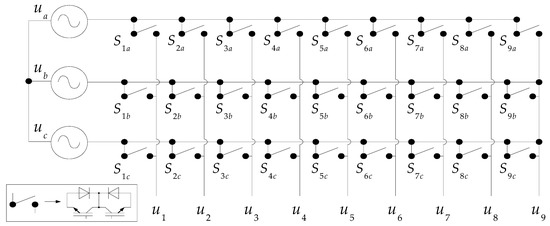
Figure 1.
Scheme of the three-to-nine-phase multiphase matrix converter (MC) topology. Inputs are named ua, ub, uc, and outputs are named u1–u9.
The output voltage waveforms in the MC are composed of segments of sequentially chosen parts of input voltage waves. Therefore, the existence functions defined in [38] was used to describe the operation of the MC switching matrix. According to [38,39] these functions at any given time can have either unit or zero amplitude. The authors of [39] suggest that it is more appropriate to call the “existence function” as a “modulation function”. Further, the existence function is named as a switching function Snl (1) and determines conduction state of each bidirectional switch.
where Snl is the switching function, n the output phase and l the input phase.
The relation between instantaneous value of the output voltage uo and instantaneous value of the input voltage ui is defined in terms of switching functions (2). A similar situation arises when considering a relation between the input current ii and the output current io (3).
where S is the transfer matrix and ST the transpose of the matrix S
The RMS value of the output voltage in the three-to-nine-phase MC can reach up to 76,16% of the input voltage [40].
3. Switching Configurations in the Three-to-Nine-Phase MC
There are 227 possible switching configurations resulting from the two-state work of switches, but only 39 switching configurations are allowed to be used. This limitation results from the nature of the power source at the input of the MC and the nature of the load. Input phases should not be short circuited together, and output phases should not be interrupted under any condition, due to the presence of an inductive load. The switching combinations of the connection between the nine output phases and the three input phases in the MC can be analyzed in twelve groups (Table 1). Each of these twelve groups contain three or six sub-groups. The names of the switching combinations in sub-groups are {x,y,z}, where x, y and z represent the number of the output phases connected to input phases a, b and c, respectively. For example, in group number 4 one of the sub-group is {7,1,1}, which means that seven output phases are connected to the input phase a, one output phase is connected to the input phase b, and one output phase is connected to the input phase c.

Table 1.
Rotating space vectors in the three-to-nine-phase MC.
The analysis of all twelve groups allows to notice that only switching states from the group number 12 can be used in elimination of the CMV. The CMV for nine output phases equals zero when all of the three input phases take part in synthesizing the output voltage. To each input phase a, b and c, any three of nine output phases have to be connected. This statement is correct when considering the balanced and sinusoidal input voltage.
4. Output Voltage Space Vectors Eliminating the CMV
The output voltage of the three-to-nine-phase MC can be represented by usage of space vectors (4).
where .
Each of the instantaneous output voltages, u1, u2, u3, u4, u5, u6, u7, u8 and u9, is connected to the one of the input phase voltages ua, ub or uc. The subscript “xxxxxxxxx” in the name means appropriately the name of input phase chosen into output phases 1, 2, 3, 4, 5, 6, 7, 8 and 9, for example, output voltage space vector . Assuming that the three-to-nine-phase MC is supplied by balanced input voltage (5), the rotating voltage space vector could be seen as counterclockwise (CCW) or clockwise (CW) rotating space vector.
where Uim is the amplitude of input voltage and ωi the angular frequency of input voltage.
The CCW and CW rotating space vectors can be defined as (6) or (7). A phase shift between each of CCW or CW space vectors is 120°.
where .
Output voltage space vector representing a nine-phase output voltage (4) can be transformed to a geometrical sum of input voltage space vectors (8). In (8), vectors named , and are voltage space vectors representing output voltage for three phases appropriately indicted in the subscripts. Those vectors can be CCW or CW rotating space vectors, and they can be described by equations from (6) or (7), respectively. The subscript, e.g., “147” in the name means appropriately the name of chosen output phases 1, 4 and 7.
The CMV is eliminated only when the input and output space vectors are rotating space vectors. When , and are rotating vectors, then output space vector is a rotating vector too.
Performing a space vector analysis in Section 3, turned out to be helpful to find out which switching states from the group number 12 should be used for eliminating the CMV.
Among 1680 switching combinations there are:
- 1458 combinations for the output voltage space vectors with variable both module and phase angle on the complex plane;
- 162 combinations for active output voltage space vectors with variable modules and fixed phase angle on the complex plane;
- 54 combinations for the output voltage represented by rotating voltage space vectors with constant module and constant angular speed on complex plane;
- 6 combinations for zero output voltage space vectors.
For the CMV elimination in the three-to-nine phase MC, 54 rotating vectors from the group 12 can be used in modulation method. These 54 rotating output voltage space vectors can be divided into three groups due to the values of modules (Table 2). A phase shift between space vectors in each group is 40°.
Table 2.
Rotating space vectors of group 12 resulting in elimination of the common mode voltage (CMV).
Space vectors presented in Table 2 divided into counterclockwise (CCW) and clockwise (CW) rotating vectors are shown in Figure 2. It could be noted that direction of the rotation is the only difference between space vectors in each group, because the length and initial phase angle are the same.
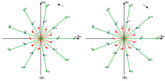
Figure 2.
Initial arrangement on complex plane of rotating voltage space vectors that are used to eliminate the CMV in the three-to-nine-phase MC: (a) CCW; (b) CW.
The application of the chosen rotating voltage space vectors in modulation of the switch duty cycles results in the zero CMV according to the formula (9).
For example, the CMV for a rotating space vector equals 0 (10).
5. Method of Modulation
To realize a synthesis of the output voltage with application of rotating voltage space vectors, carrier-based implementation of the SVM is used. Venturini modulation functions [3] are utilized to set out the switch duty cycles Snl. For the three-to-nine-phase MC with both symmetric sinusoidal input and output voltages, with output amplitude and angular frequency indicated as Uo, ωo, the Venturini modulation functions are indicated in relationships (11,12,13). The utilization of those modulation functions (11,12,13) results in maximum voltage transfer ratio kU = 0.5 and possibility to control of the input displacement angle in the range: −φo < φi < φo.
It can be noted that when the MC synthesizes the output and input waveforms, and the input displacement angle is (), there are nine groups consisting of three identical modulation functions (14). It is similar in case of () (15). The implementation of the carrier-based SVM allows for arbitrariness in switching duty cycles order for the switching period Ts. The same waveform of some modulation functions enables such arrangement of the switch duty cycles during Ts, that ensures utilization of the rotating voltage space vectors only. Modulation functions defined in (14) give output voltages represented by CCW rotating voltage space vectors and lagging input displacement angle. Modulation functions presented in (15) give output voltages represented by CW rotating voltage space vectors and leading input displacement angle. Further the modulation method with the use of the CCW modulation functions is named CCW method and CW method when the CW modulation functions are used.
The block diagram of the carrier based SVM modulation strategy for output phase number “1” is shown in Figure 3. The CCW modulation method is realized, so the modulation functions (14) are used to find the discreet switching functions S1a, S1b and S1c. Application of the CCW method, using CCW rotating voltage space vectors to eliminate the CMV, demands an assumption that the parameters α1 = 1 and α2 = 0. Maximum value of the voltage transfer ratio kU(max) = 0.5.
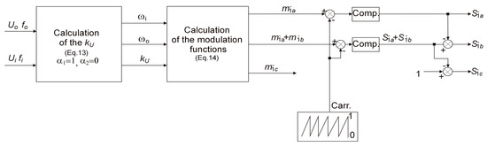
Figure 3.
Block diagram of the currier based CCW modulation for output phase number “1”.
The exemplary configuration of switch duty cycles during the period Ts is presented in Figure 4. Carrier and modulating signals are compared to show switching combinations. Numbers from 1 to 7 in Figure 4 correspond to the rotating voltage space vectors that are created for certain switching states.
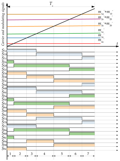
Figure 4.
Switch duty cycles in the three-to-nine-phase MC for CCW method. Numbers from 1 to 7 respond the rotating voltage space vectors , , ,, , and , respectively. Simulation performed for output frequency 30 Hz and voltage transfer ratio kU = 0.5.
6. Simulation Results
For confirmation of theoretical and analytical investigations, the simulations of analyzed converter were performed using the three-to-nine-phase MC model prepared in ATP software. In Figure 5, power circuit of the tested converter is presented. The bidirectional switches are assumed to be ideal. In ATP, they are represented by time-controlled switches. The ideal sinusoidal three-phase voltage source is used as a supply. The nine-phase resistive-inductive load is used in the simulation model.
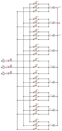
Figure 5.
ATP simulation model of the three-to-nine-phase MC supplying nine-phase load. Input voltages are named Ua, Ub and Uc, output voltages are named from U1 to U9.
The control with application of the carrier-based SVM with Venturini modulation functions is considered. In the Section 5 two methods, CCW method and CW method, are distinguished. For each of those methods the Venturini functions are different. Thus, it is possible to perform simulations by using CCW (14) or CW method (15).
The voltage difference between the star point of the load and the ground potential represents the CMV of this converter topology.
Parameters of the source, load and control, that were used in the three-to-nine-phase MC simulation model are presented in the Table 3.
Table 3.
Parameters of the three-to-nine-phase MC simulation model.
Two SVM control methods are tested: CCW method and CW method. The first method is realized with the use of modulation functions (13) and the CCW rotating voltage space vectors. It results in a lagging input displacement angle (Figure 6a). The second method utilizes the modulation functions (14) and the CW rotating voltage space vectors, which causes leading displacement angle (Figure 6b).
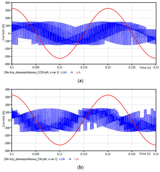
Figure 6.
Input voltage (red) and current (blue) waveforms of phase a for (a) CCW method; (b) CW method.
Fourier analysis of input current of phase a was performed and is presented in Figure 7. The analysis was carried out with an accuracy of 10 Hz. For instance, 500th harmonic in Figure 7 should be treated as a component with a frequency equal 5 kHz. It is shown that not only the fundamental but also higher-order harmonics related to the switching frequency are present.
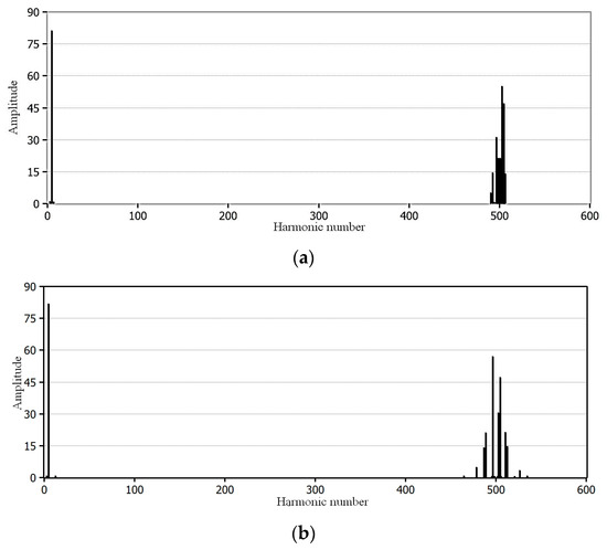
Figure 7.
Fourier analysis of input current of phase a for (a) CCW method and (b) CW method.
In Figure 8, the waveforms of output currents of phases from 1 to 9 are presented. The waveforms are exactly the same for the CCW method and the CW method. It can be noted that the currents are sinusoidal and the phase shift between each of phase output current is 40° (Figure 8).
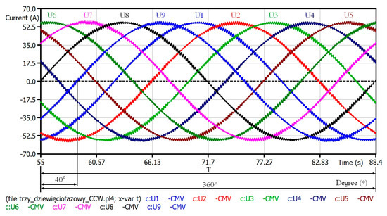
Figure 8.
Waveforms of the output currents of phases from 1 to 9 for the CCW method and the CW method.
It is shown in simulation results that the CMV elimination in the three-to-nine-phase MC is achieved (Figure 9). For both CCW method (Figure 9a) and CW method (Figure 9b), the zero CMV is achieved although the phase voltage is synthesized as short modulated in time pulses equal to instantaneous input phase voltage. In the Fourier analysis of the phase output voltage (Figure 10), it is showed that in addition to the fundamental, component waveforms contain harmonics centered around the switching frequency.
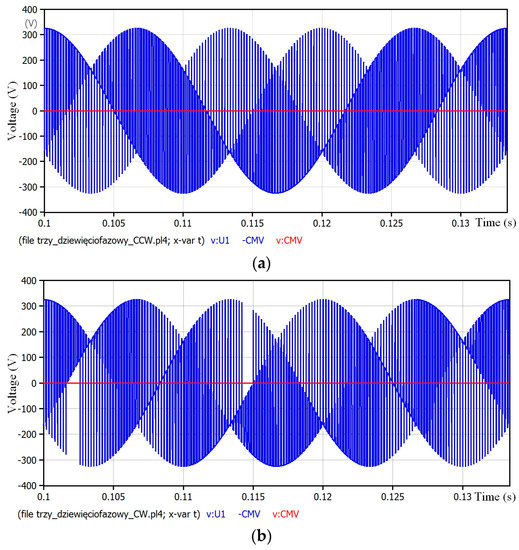
Figure 9.
Waveforms of the phase output voltage (blue lines) and the CMV (red line) for (a) CCW method and (b) CW method. Simulation performed for the output frequency fo = 30 Hz.
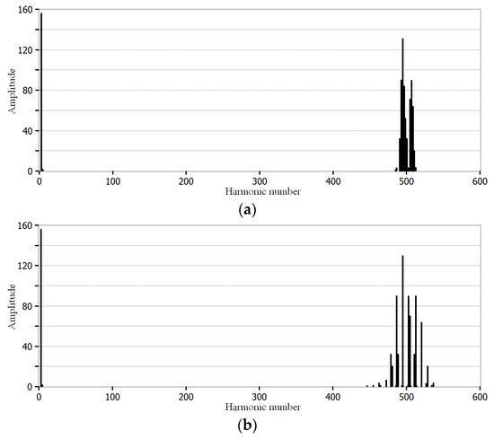
Figure 10.
Fourier analysis of phase output voltage for (a) CCW method and (b) CW method.
For the elimination of the CMV only rotating output space vectors are used. To show the participation of the rotating voltage space vectors from particular groups (Table 2) in the synthesis of the output voltage, the simulations for different values of the output frequency fo and voltage transfer ratio kU were performed. Simulation results received for the voltage transfer ratio kU = 0.5 and different values of the output frequency were performed for the CCW method (Figure 11) and the CW method (Figure 12) for one period of output frequency. Additionally, in Figure 11, the rotating voltage space vectors from group I, II and III are pointed out to make it easy to notice their trajectory. It could be seen that the participation of the rotating voltage space vectors from particular groups depends on the relation between the input and the output frequency. It can be noted that for various values of the output frequency, not all of the rotating voltage space vectors take part in the synthesis of the output voltage. When the output frequency equals the input one, rotating voltage space vectors from groups I and III are used. The rotating voltage space vectors from all three groups are used, when the output frequency is different than input frequency. Analysis of the simulation results for different values of the voltage transfer ratio and fixed output frequencies do not change this regularity (Figure 13 and Figure 14).
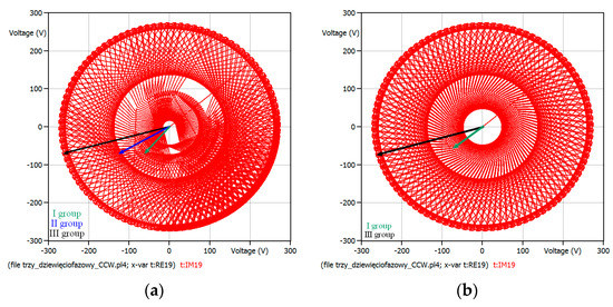
Figure 11.
Trajectory of the output voltage rotating space vector for output frequency: (a) 30 Hz and (b) 50 Hz. Simulations performed for the voltage transfer ratio kU = 0.5, for one period of output frequency and CCW method.
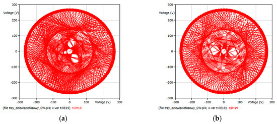
Figure 12.
Trajectory of the output voltage rotating space vector for output frequency: (a) 30 Hz; (b) 50 Hz. Simulations performed for the voltage transfer ratio kU = 0.5, for one period of output frequency and CW method.
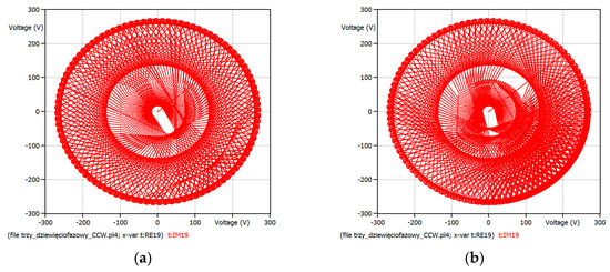
Figure 13.
Trajectory of the output rotating voltage space vector for the voltage transfer ratio: (a) kU = 0.1 and (b) kU = 0.5. Simulations performed for the output frequency fo = 30 Hz, for one period of output frequency and CCW method.
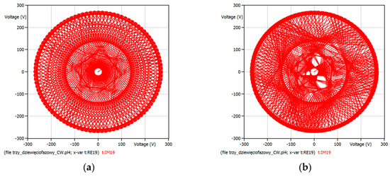
Figure 14.
Trajectory of the output rotating voltage space vector for the voltage transfer ratio: (a) kU = 0.1; (b) kU = 0.5. Simulations performed for the output frequency fo = 30 Hz, for one period of output frequency and CW method.
7. Conclusions
The DMC is an important converter topology with characteristics such as simple power circuit, output voltage with variable amplitude and frequency, lack of DC-link capacitor, regeneration ability and both sinusoidal source and load currents. Moreover, an important advantage of the DMC is that the zero CMV can be realized without any hardware.
In this paper, it is assumed that the bidirectional switches are ideal and with zero on and off switching time. Therefore, there is no need to consider a commutation strategy.
The carrier-based SVM with Venturini modulation functions has been successfully used for the CMV elimination in the three-to-nine-phase DMC. The carrier-based SVM method does not need any complicated calculations and is quite simple. Two modulation methods were investigated: the CCW method and the CW method. Both of them result in synthesis of nine-phase output voltage consisting of fundamental component and high frequency components concentrated near multiple of switching frequency. In both methods, the zero CMV is achieved. In synthesis of the output voltage, complete elimination of CMV is accomplished using the rotating voltage space vectors only. Analysis of all possible configurations in the three-to-nine-phase MC is helpful to find 54 rotating voltage space vectors with constant module and constant angular speed on complex plane that could be used to eliminate the CMV. The use of Venturini modulation functions automates the choose of appropriate vectors out of 54 distinguished ones in proposed carrier-based CCW and CW modulation methods. A carrier-based implementation of the SVM by using rotating voltage space vectors only is an alternative way to achieve the SVM that avoids trigonometric and division operations that could be needed to implement the SVM using the general vector approach.
In the simulation results, it can be noted that only rotating voltage space vectors are used to eliminate the CMV. Depending on the value of the output frequency and referenced output voltage, not all of the rotating voltage space vectors are used. Nevertheless, the zero CMV is achieved in any case.
Since the difference between the CCW and CW rotating voltage space vectors is a direction of rotation, the CCW method results in lagging input displacement angle, and the CW method gives leading input displacement angle, which was proved by simulation results. The presented CCW method and the CW method that is implemented for the elimination of the CMV do not allow to control the phase shift between input voltage and current. However, the use of both Venturini modulation functions together makes it possible to control this value. This aspect will be investigated in future research.
Author Contributions
Conceptualization, J.R.; methodology, J.R.; software, E.S. and J.R.; formal analysis, E.S. and J.R.; investigation, E.S. and J.R.; writing—original draft preparation, E.S.; writing—review and editing, E.S. and J.R.; visualization, E.S. and J.R.; supervision, J.R. All authors have read and agreed to the published version of the manuscript.
Funding
This research received no external funding.
Conflicts of Interest
The authors declare no conflict of interest
References
- Empringham, L.; Kolar, J.W.; Rodriguez, J.; Wheeler, P.W.; Clare, J.C. Technological Issues and Industrial Application of Matrix Converters: A Review. IEEE Trans. Ind. Electr. 2013, 60, 4260–4271. [Google Scholar] [CrossRef]
- Zhang, J.; Li, L.; Dorrell, D. Control and Applications of Direct Matrix Converters: A Review. Chin. J. Electr. Eng. 2018, 4, 18–27. [Google Scholar]
- Ali, M.; Iqbal, A.; Khan, R.; Ayyub, M.; Anees, M. Generalized Theory and Analysis of Scalar Modulation Techniques for a m x n Matrix Converter. IEEE Trans. Power Electron. 2017, 32, 4864–4877. [Google Scholar] [CrossRef]
- Rodriguez, J.; Rivera, M.; Kolar, J.W.; Wheeler, P.W. A Review of Control and Modulation Methods for Matrix Converters. IEEE Trans. Ind. Electr. 2012, 59, 58–70. [Google Scholar] [CrossRef]
- Trentin, A.; Zanchetta, P.; Empringham, L.; de Lillo, L.; Wheeler, P.; Clare, J. Experimental Comparison Between Direct Matrix Converter and Indirect Matrix Converter Based on Efficiency. In Proceedings of the 2015 IEEE Energy Conversion Congress and Exposition (ECCE), Montreal, Canada, 20–24 September 2015. [Google Scholar]
- Jussila, M.; Tuusa, H. Comparision of Direct and Indirect Matrix Converters in Induction Motor Drive. In Proceedings of the IECON 2006-32nd Annual Conference on IEEE Industrial Electronics, Paris, France, 6–10 November 2006. [Google Scholar]
- Kolar, J.W.; Friedli, T.; Rodriguez, J.; Wheeler, P.W. Review of Three-Phase PWM AC-AC Converter Topologies. IEEE Trans. Ind. Electr. 2011, 58, 4988–5006. [Google Scholar] [CrossRef]
- Abdel-Rahim, O.; Abu-Rub, H.; Kouzou, A. Nine-to-Three Phase Direct Matrix Converter with Model Predictive Control for Wind Generation System. Energy Procedia 2013, 42, 173–182. [Google Scholar] [CrossRef]
- Abdel-Rahim, O.; Ali, Z.M. Control of Seven-to-Three Phase Direct Matrix Converter Using Model Predictive Control for Multiphase Wind Generation. In Proceedings of the 2014 16th International Conference on Harmonics and Quality of Power (ICHQP), Bucharest, Romania, 25–28 May 2014. [Google Scholar]
- Yamamoto, E.; Hara, H.; Uchino, T.; Kawaji, M.; Kume, T.J.; Kang, J.K.; Krug, H.P. Development of MCs and its Applications in Industry. IEEE Ind. Electron. Mag. 2011, 5, 4–12. [Google Scholar] [CrossRef]
- Kang, J.; Kume, T.; Hara, H.; Yamamoto, E. Common-mode voltage characteristics of matrix converter-driven AC machines. In Proceedings of the Fourtieth IAS Annual Meeting. Conference Record of the 2005 Industry Applications Conference, Kowloon, Hong Kong, China, 2–6 October 2005; Volume 4, pp. 2382–2387. [Google Scholar]
- Vijayagopal, M.; Empringham, L.; de Lillo, L.; Tarisciotti, L.; Zanchetta, P.; Wheeler, P. Control of a direct matrix converter induction motor drive with modulated model predictive control. In Proceedings of the 2015 IEEE Energy Conversion Congress and Exposition (ECCE), Montreal, Canada, 20–24 September 2015; pp. 4315–4321. [Google Scholar]
- Gupta, R.K.; Mohapatra, K.K.; Somani, A.; Mohan, N. Direct-Matrix-Converter-Based Drive for a Three-Phase Open-End-Winding AC Machine with Advanced Features. IEEE Trans. Ind. Electr. 2010, 57, 4032–4042. [Google Scholar] [CrossRef]
- Zhang, J.; Li, L.; Dorrell, D.; Guo, Y. Direct Torque Control with a Modified Switching Table for a Direct Matrix Converter based AC Motor Drive System. In Proceedings of the 2017 20th International Conference on Electrical Machines and Systems (ICEMS), Sydney, Australia, 11–14 August 2017; pp. 1–6. [Google Scholar]
- Munuswamy, I.; Wheeler, P.W. Matrix Converter for More Electric Aircraft; IntechOpen: London, UK, 2019. [Google Scholar]
- Levi, E.; Bojoi, R.; Profumo, F.; Toliyat, H.A.; Williamson, S. Multiphase induction motor drives–a technology status review. IET Electr. Power Appl. 2007, 1, 489–516. [Google Scholar] [CrossRef]
- Ahmed, S.M.; Iqbal, A.; Abu-Rub, H.; Rodriguez, J.; Rojas, C.; Saleh, M. Simple Carrier-Based PWM Technique for a Three-to-Nine-Phase Direct AC-AC Converter. IEEE Trans. Ind. Electr. 2011, 58, 5014–5023. [Google Scholar]
- Dabour, S.M.; Allam, S.M.; Rashad, E.M. Indirect Space-Vector PWM Technique for Three to Nine Phase Matrix Converters. In Proceedings of the IEEE GCC Conference and Exhibition, Muscat, Oman, 1–4 February 2015. [Google Scholar]
- Kalaiselvi, J.; Srinivas, S. Bearing Currents and Shaft Voltage Reduction in Dual-Inverter-Fed Open-End Winding Induction Motor with Reduced CMV PWM Methods. IEEE Trans. Ind. Electr. 2015, 62, 144–152. [Google Scholar] [CrossRef]
- Ahmed, S.; Abu-Rub, H.; Salam, Z. Common-Mode Voltage Elimination in a Three-to-Five-Phase Dual Matrix Converter Feeding a Five-Phase Open-End Drive Using Space-Vector Modulation Technique. IEEE Trans. Ind. Electr. 2015, 62, 6051–6063. [Google Scholar] [CrossRef]
- Dabour, S.M.; Abdel-Khalik, A.S.; Ahmed, S.; Massoud, A. Common-Mode Voltage Reduction of Matrix Converter fed Seven-Phase Induction Machine. In Proceedings of the 2016 XXII International Conference on Electrical Machines (ICEM), Lausanne, Switzerland, 4–7 September 2016. [Google Scholar]
- Rząsa, J. Control of a matrix converter with reduction of a common mode voltage. In Proceedings of the IEEE Compatibility in Power Electronics, Gdynia, Poland, 12–15 September 2005. [Google Scholar]
- Mohapatra, K.K.; Ned, M. Open-End Winding Induction Motor Driven with Matrix Converter for Common-Mode Elimination. In Proceedings of the International Conference on Power Electronics, Drives and Energy Systems, New Delhi, India, 12–15 December 2006. [Google Scholar]
- Rząsa, J. Research on Dual Matrix Converter Feeding an Open-End-Winding Load Controlled with the Use of Rotating Space Vectors. Part I. In Proceedings of the IECON 2013-39th Annual Conference of the IEEE Industrial Electronics Society, Vienna, Austria, 10–13 November 2013. [Google Scholar]
- Rząsa, J.; Garus, G. Research on Dual Matrix Converter Feeding an Open-End-Winding Load Controlled with the Use of Rotating Space Vectors. Part II. In Proceedings of the IECON 2013-39th Annual Conference of the IEEE Industrial Electronics Society, Vienna, Austria, 10–13 November 2013. [Google Scholar]
- Baranwal, R.; Basu, K.; Mohan, N. An Alternative Carrier based implementation of Space Vector PWM for Dual Matrix Converter Drive with Common Mode Voltage Elimination. In Proceedings of the IECON 2014-40th Annual Conference of the IEEE Industrial Electronics Society, Dallas, TX, USA, 29 October–1 November 2014. [Google Scholar]
- Rząsa, J. An Alternative Carrier-Based Implementation of Space Vector Modulation to Eliminate Common Mode Voltage in a Multilevel Matrix Converter. Electronics 2019, 8, 190. [Google Scholar] [CrossRef]
- Rząsa, J.; Sztajmec, E. Elimination of Common Mode Voltage in Three-To-Six-Phase Matrix Converter. Energies 2019, 12, 1662. [Google Scholar] [CrossRef]
- Nguyen, N.H.; Lee, H.H. A Modulation Scheme for Matrix Converters with Perfect Zero Common-Mode Voltage. IEEE Trans. Power Electron. 2016, 31, 5411–5422. [Google Scholar] [CrossRef]
- Lei, J.; Feng, S.; Zhou, B.; Nguyen, H.; Zhao, J.; Chen, W. Simple Modulation Scheme with Zero Common-Mode Voltage and Improved Efficiency for Direct Matrix Converter Fed PMSM Drives. IEEE J. Emerg. Sel. Top. Power Electron. 2019. [Google Scholar] [CrossRef]
- Wang, D.; Tang, S.; Wang, J.; Xiong, Z.; Mo, S.; Yin, X.; Shuai, Z.; Shen, Z.J. Commutation Strategies for Single-Chip Dual-Gate Bidirectional IGBTs in Matrix Converters. In Proceedings of the 2016 IEEE Energy Conversion Congress and Exposition (ECCE), Milwaukee, WI, USA, 18–22 September 2017. [Google Scholar]
- Wang, L.; Dan, H.; Zhao, Y.; Zhu, Q.; Peng, T.; Sun, Y.; Wheeler, P. A Finite Control Set Model Predictive Control Method for Matrix Converter with Zero Common-Mode Voltage. IEEE J. Emerg. Sel. Top. Power Electron. 2017, 6, 327–338. [Google Scholar] [CrossRef]
- Linhart, L.; Lettl, J.; Bauer, J. Matrix Converter Two-Step Commutation Method Limitations. In Proceedings of the 14th International Power Electronics and Motion Control Conference EPE-PEMC 2010, Ohrid, Macedonia, 6–8 September 2010. [Google Scholar]
- Hao, L.; Ziling, N.; Ye, Z. A New Controlled Commutation Strategies for Matrix Converter. In Proceedings of the 2008 International Symposium on Computer Science and Computational Technology, Shanghai, China, 20–22 December 2008. [Google Scholar]
- Hendawi, E.; Khater, F.; Shaltout, A. Analysis, Simulation and Implementation of the Space Vector Pulse Width Modulation Inverter. In Proceedings of the 9th WSEAS International Conference on Applications of Electrical Engineering, Rodos, Greece, 22–24 July 2009. [Google Scholar]
- Alesina, A.; Venturini, M. Analysis and Design of Optimum-Amplitude Nine-Switch Direct AC-AC. IEEE Trans. Power Electron. 1989, 4, 101–112. [Google Scholar] [CrossRef]
- Alesina, A.; Ventrurini, M. Solid-State Power Conversion: A Fourier Analysis Approach to Generalized Transformer Synthesis. IEEE Trans. Circuits Syst. 1981, 28, 319–330. [Google Scholar] [CrossRef]
- Gyugyi, L.; Pelly, B.R. Static Power Frequency Changers; John Wiley & Sons: Hoboken, NJ, USA, 1976. [Google Scholar]
- Venturini, M.; Alesina, A. The Generalised Transformer: A New Bidirectional, Sinusoidal Waveform Frequency Converter with Continuously Adjustable Input Power Factor. In Proceedings of the 1980 IEEE Power Electronics Specialists Conference, Atlanta, GA, USA, 16–20 June 1980. [Google Scholar]
- Bucknall, R.W.G.; Ciaramella, K.M. On the Conceptual Design and Performance of a Matrix Converter for Marine Electric Propulsion. IEEE Trans. Power Electr. 2010, 25, 1497–1508. [Google Scholar] [CrossRef]


© 2020 by the authors. Licensee MDPI, Basel, Switzerland. This article is an open access article distributed under the terms and conditions of the Creative Commons Attribution (CC BY) license (http://creativecommons.org/licenses/by/4.0/).