The Influence of an Interlayer on Dual Hydraulic Fractures Propagation

Abstract
1. Introduction
2. Methods
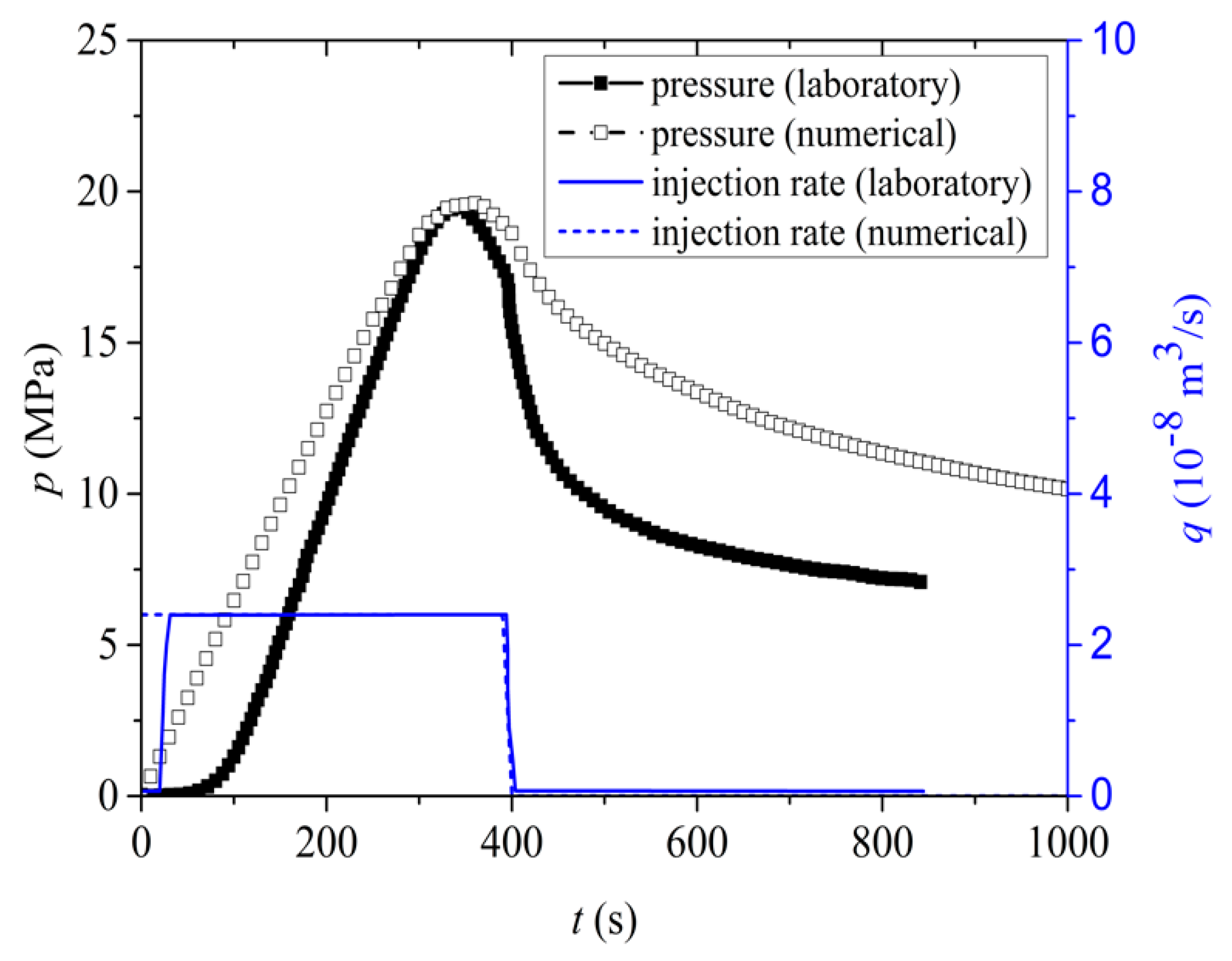
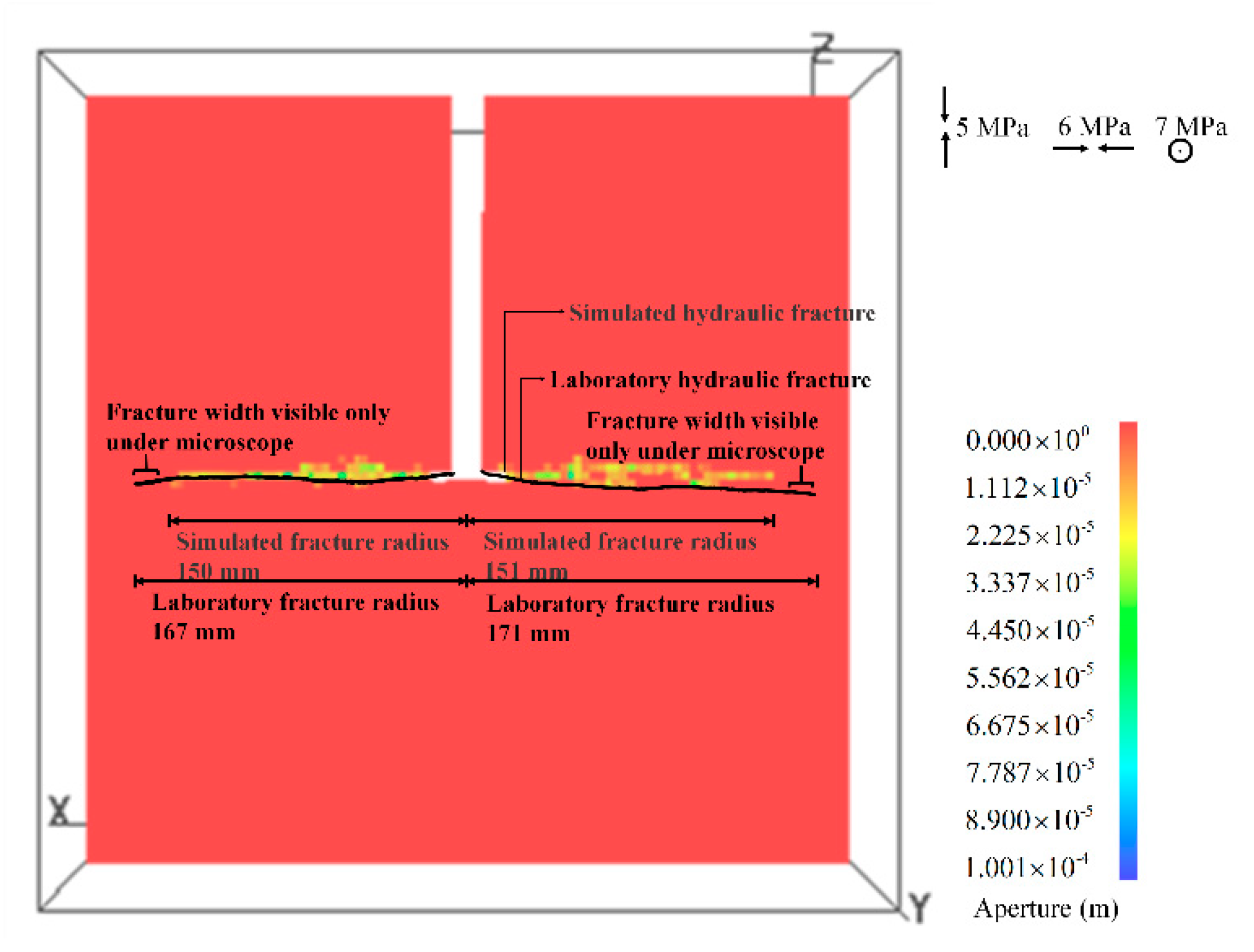
3. Validation
4. Results and Discussion
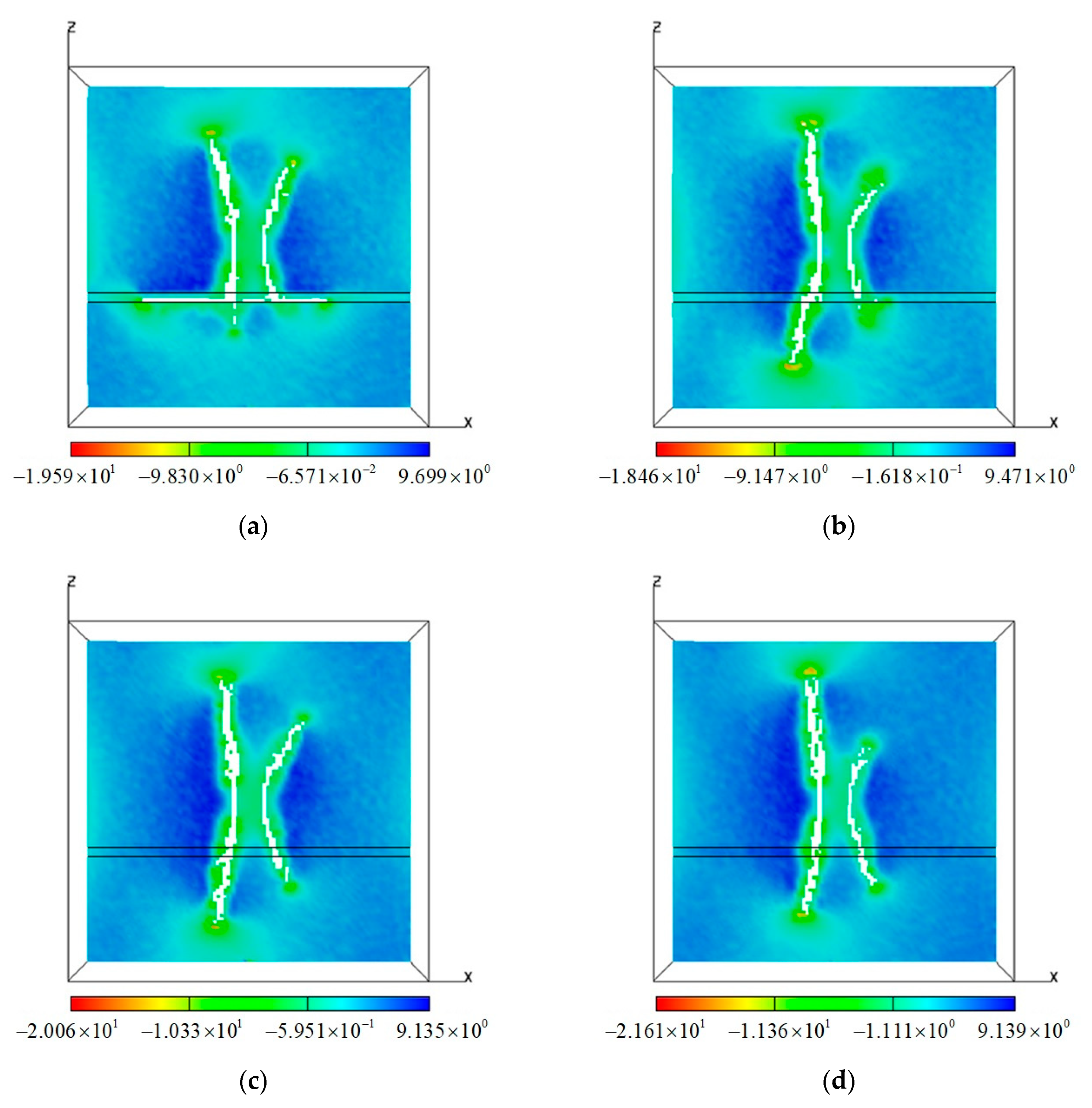
4.1. The Impact of Interlayer Properties on Dual Hydraulic Fracture Propagation in Multilayered Laboratory-Scale Models
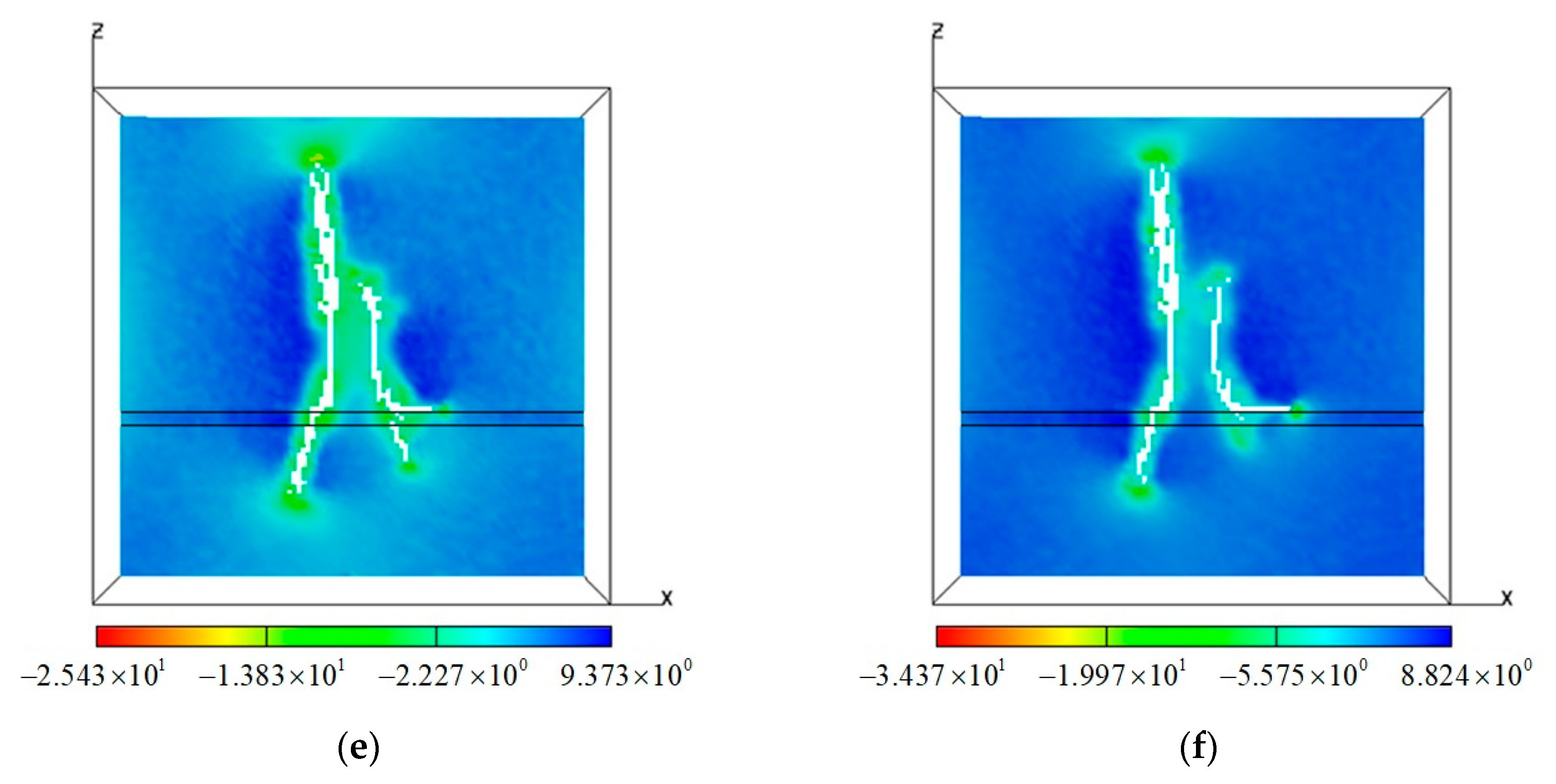
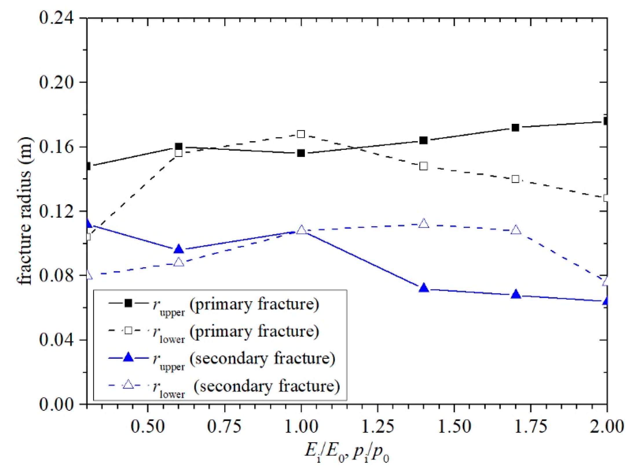
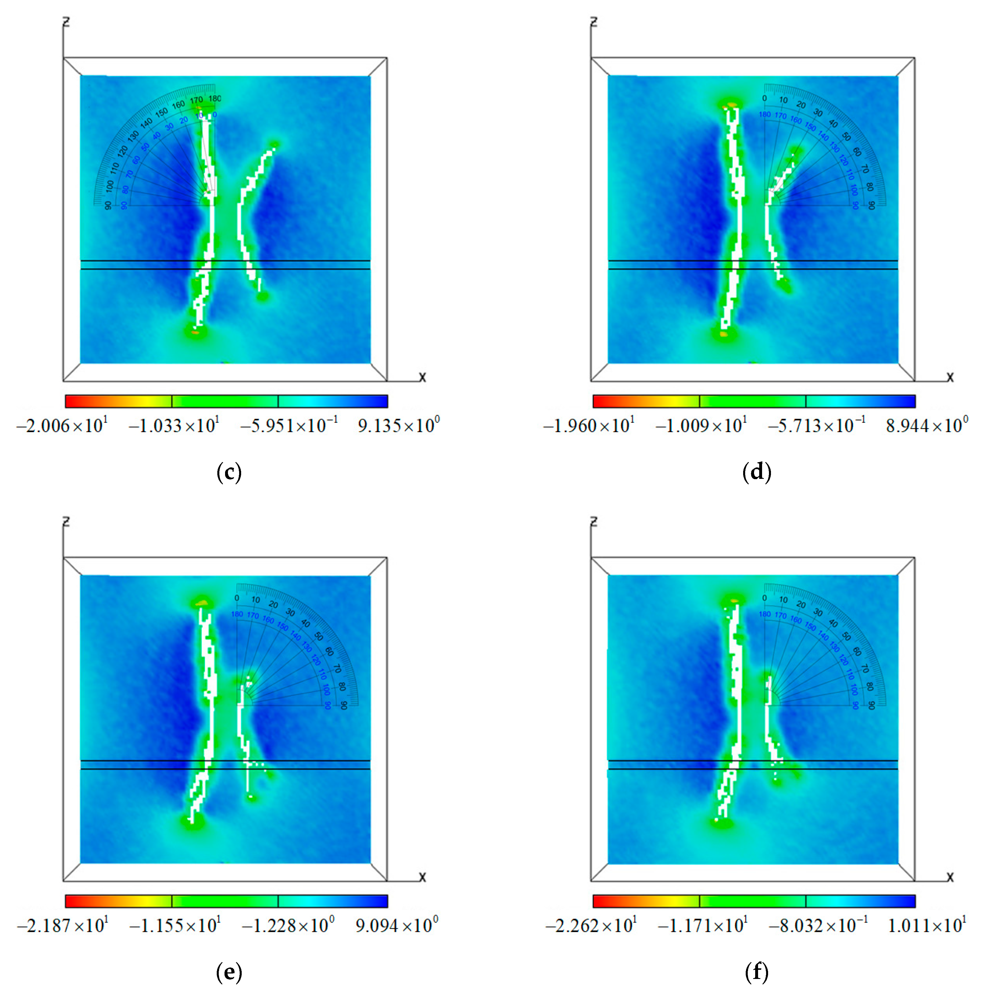
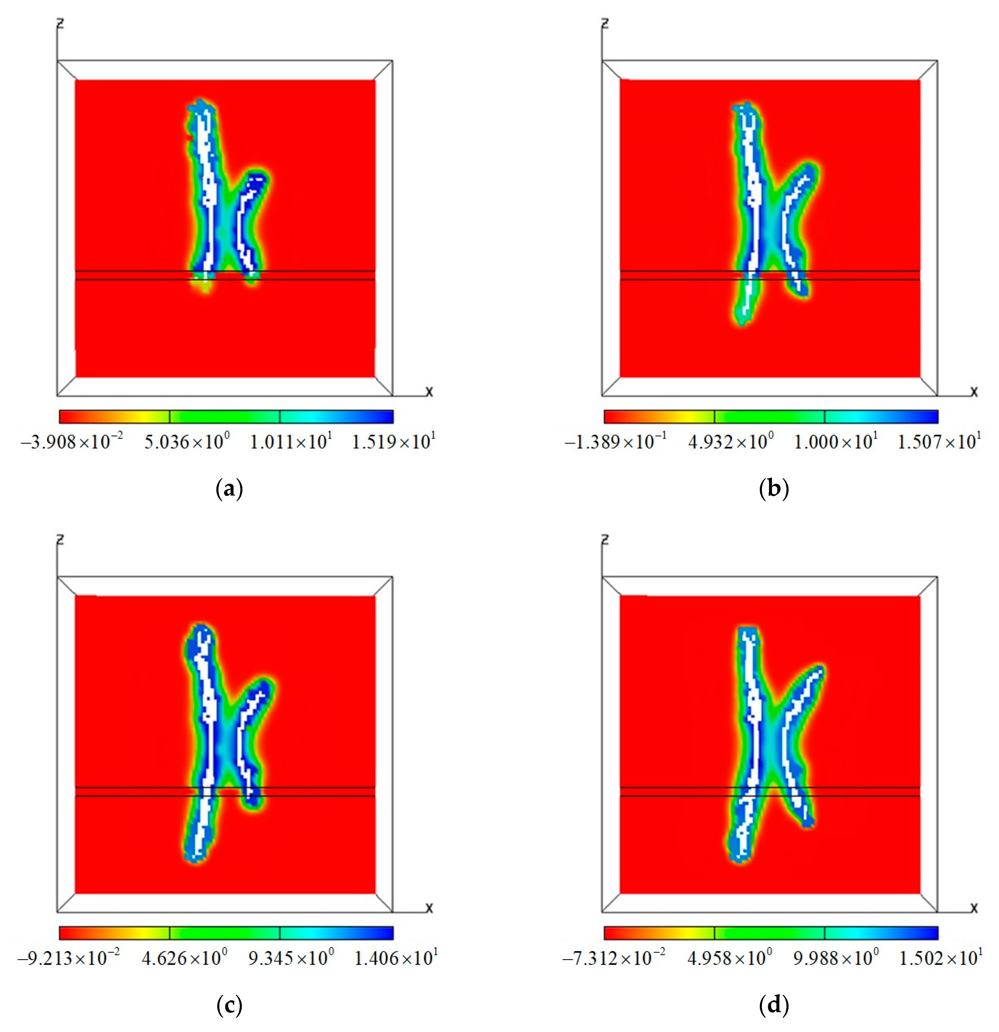
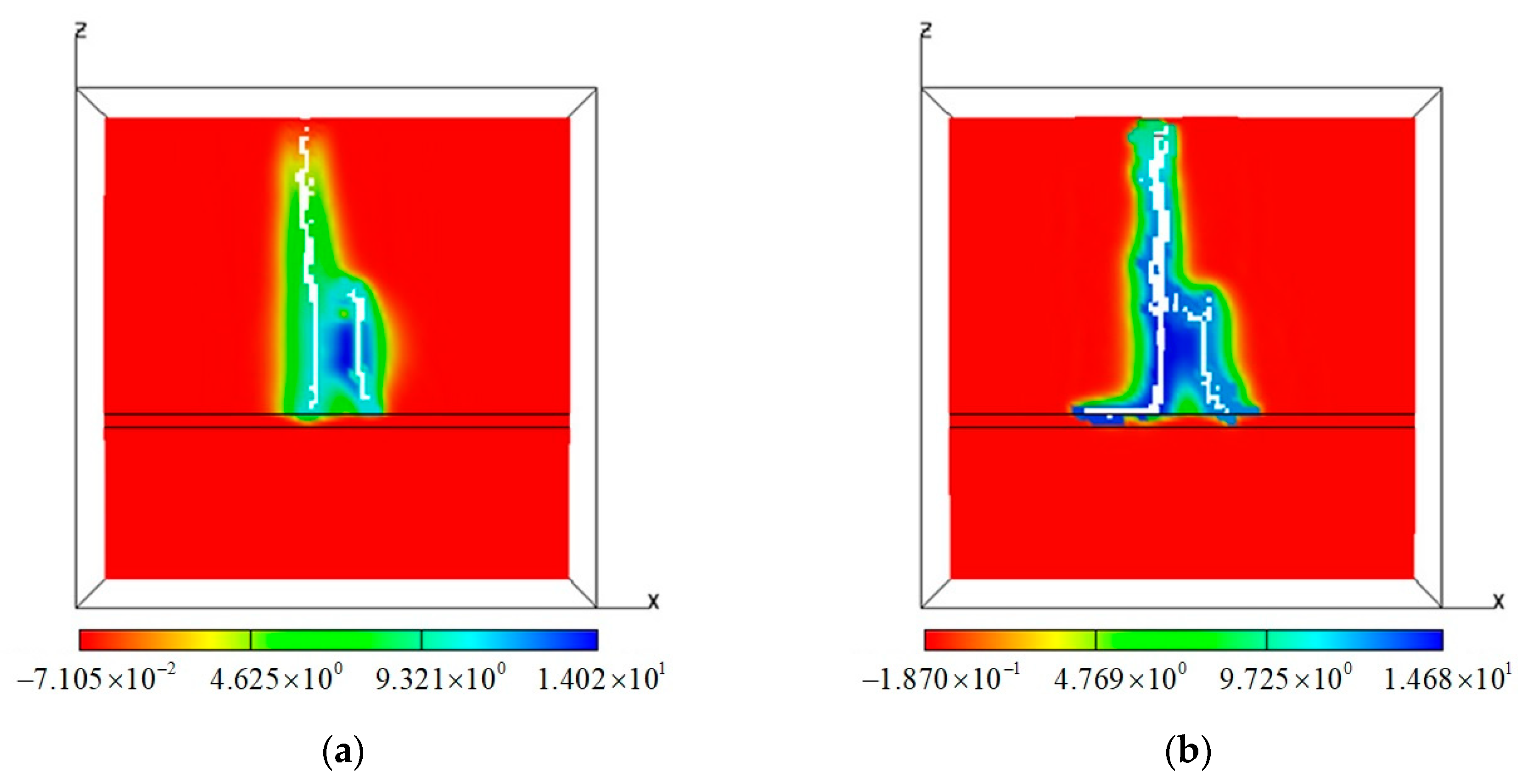
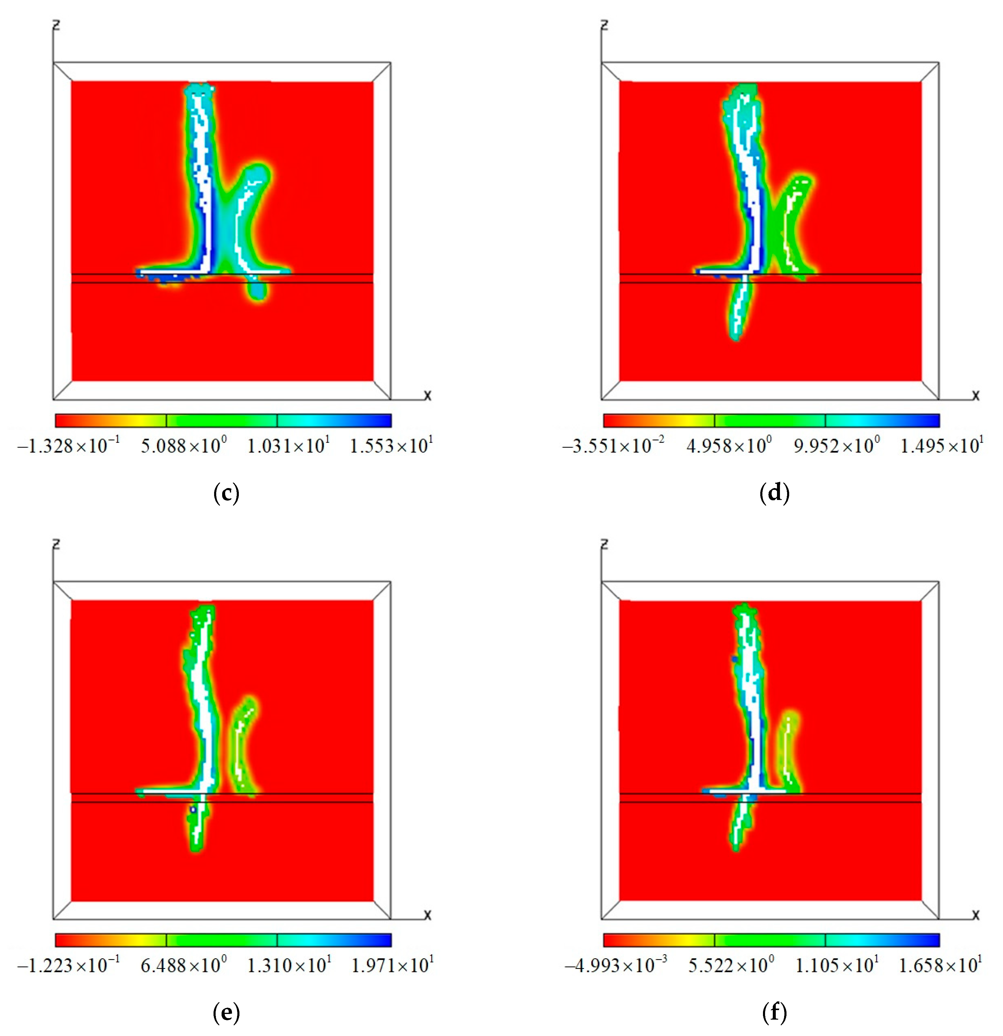
4.1.1. Sensitivity of Different Interface Young’s modulus and Strength
4.1.2. Sensitivity of Different Interface Poisson’s Ratio
4.1.3. Sensitivity of Different Interface Permeability
4.2. The Impact of Fracturing Fluid Parameters on the Propagation of Dual Hydraulic Fractures in a Multilayered Laboratory-Scale Model
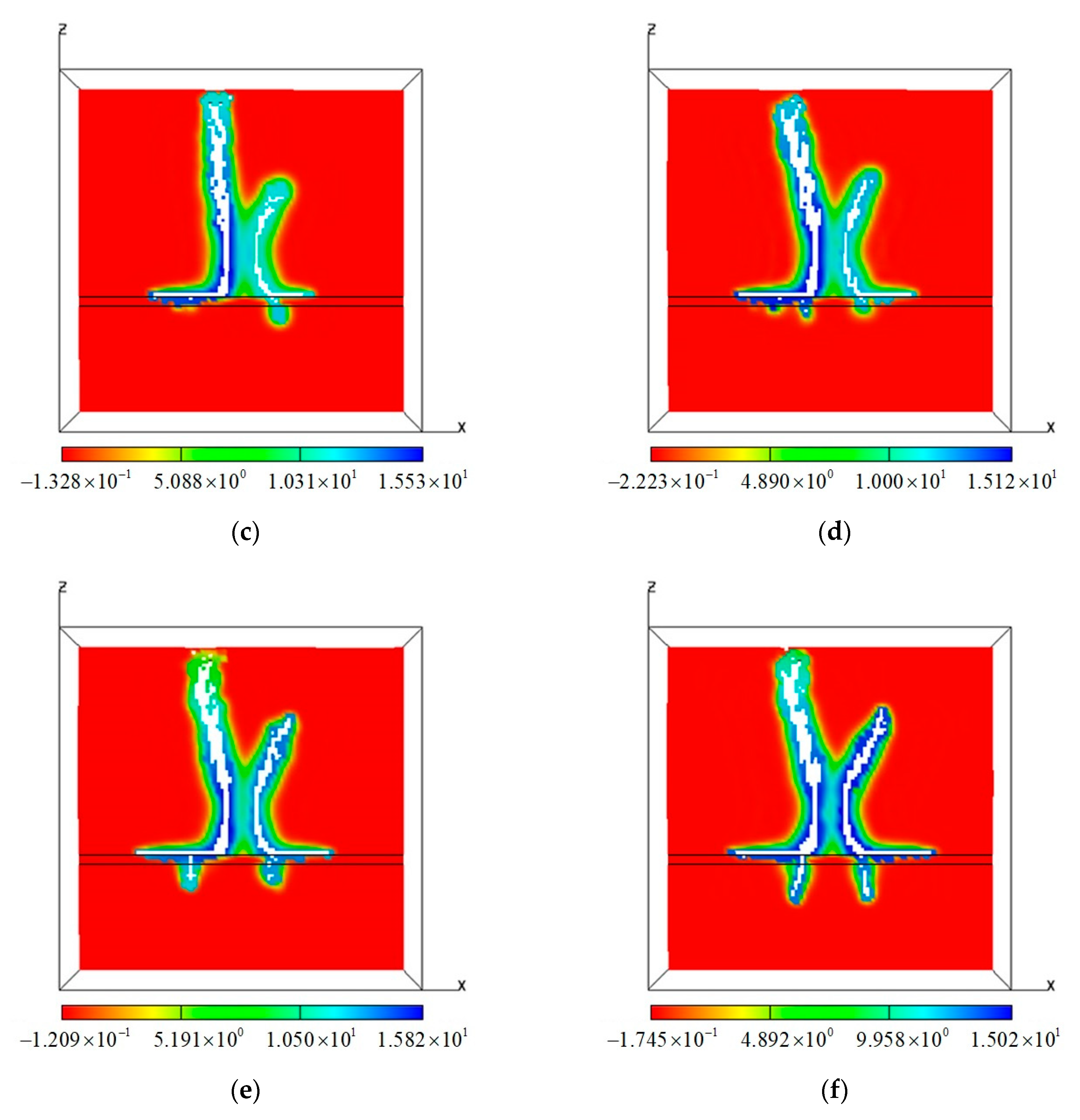
4.2.1. Sensitivity of Different Flux
4.2.2. Sensitivity of Different Fluid Viscosity
5. Conclusions
- When the mechanical properties of the interlayer are different from those of the oil-bearing layers, the interlayer has an indirect effect on the dual fractures by influencing the in situ stress distribution and has a direct influence by arresting or guiding the propagation of dual fractures.
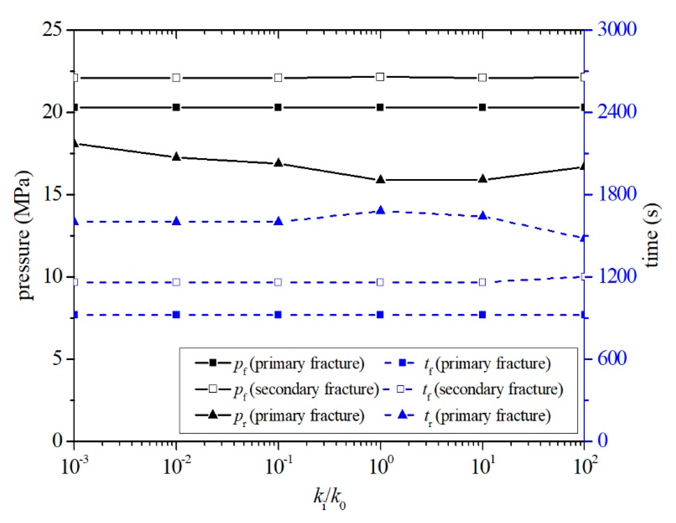
- When the permeability of the interlayer is different from those of the oil-bearing layers, the stress field will not be affected, but since the permeability changes in a range of several orders of magnitude, the permeability of the interlayer plays a key role on the dual fractures configuration and the reopening pressure of the secondary fracture.
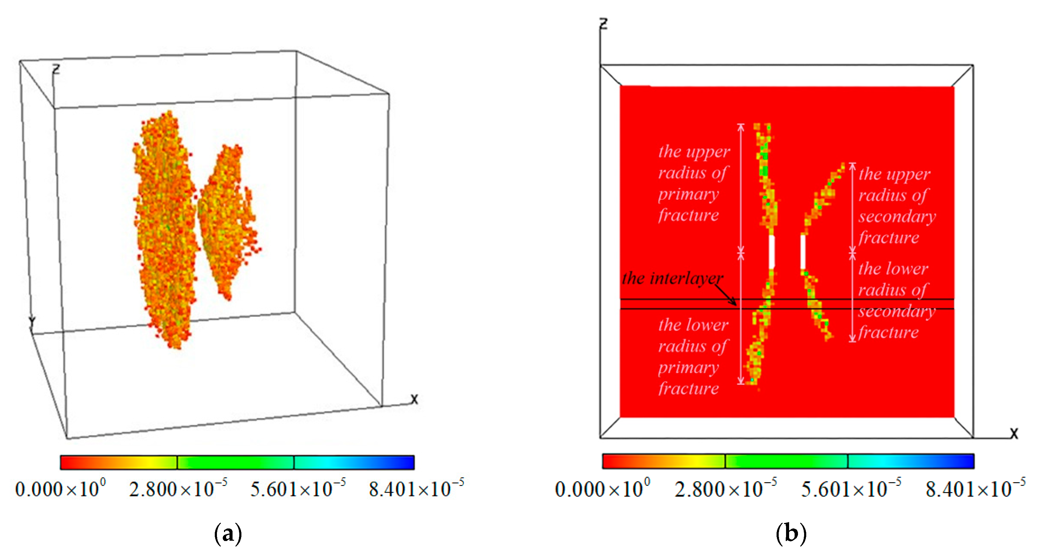
- The propagation of the secondary fracture is affected by both of the primary fracture and the interlayer. The primary fracture plays a major role in the growth of the upper part of the secondary fracture, which is far from the interlayer, while the lower part of the secondary fracture near the interlayer is predominantly controlled by the interlayer.
- When the properties of the interface are known, increasing the fracturing fluid flux is beneficial in the dual fractures crossing the interlayer. However, the fractures have branches in the horizontal direction above the interlayer, so the fluid volume is reduced after penetrating the interlayer.
- When the properties of the interface are known, increasing the fracturing fluid viscosity makes it easier for the primary fracture to cross the interlayer. Under hydraulic fracturing with a high viscosity fluid, if we shut down the injection after the initiation of the primary fracture and reopen it after the initiation of the secondary fracture, both two fractures may penetrate the interlayer.
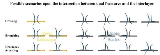
- In this paper, the interaction between dual fractures and interlayer are classified into three types for both weak layer and barrier by the primary fracture geometry as shown in Table 6. For intersection with a weak layer, the three types are:
- dual fractures cross the weak layer;
- the primary fracture branches off into the weak layer, including two patterns: (a) both fractures branch, (b) the primary fracture branches while the secondary fracture turns into the weak layer;
- dual fractures turn to propagate parallel within the bottom of weak layer, including two patterns: (a) dual fractures propagate away from each other in the weak layer without a fractured zone between them, (b) dual fractures are reoriented into the weak layer and merge into a large horizontal fractured domain.
For intersection with a barrier, the three types are:- the primary fracture crosses the barrier, including four patterns: (a) dual fractures penetrate the barrier without changing in width, (b) dual fractures penetrate the barrier with a width narrowed, (c) the primary fracture penetrates the barrier while the secondary fracture branches off above the barrier, (d) the primary fracture penetrates the barrier while the secondary fracture is reoriented to propagate parallel above the barrier.
- the primary fracture branches off above the barrier, including three patterns: (a) dual fractures branches off above the barrier, (b) the primary fracture branches off above the barrier while the secondary fracture is reoriented to propagate parallel above the barrier, (c) the primary fracture branches off above the barrier while the secondary fracture is stopped by the barrier.
- the primary fracture is arrested by the barrier, including four patterns: (a) lower parts of the dual fractures are reoriented to propagate parallel above the barrier and the upper parts of them propagate away from each other, (b) lower parts of the dual fractures reoriented to propagate parallel above the barrier and the upper part of the secondary fracture merges into the primary fracture, (c) both of the fractures are stopped by the barrier, (d) dual fractures are reoriented into the barrier and find a weak place to penetrate the barrier. Table 6 contains most of the fracture configuration when dual fractures encounter an interface.
Author Contributions
Funding
Conflicts of Interest
References
- Tang, J.Z.; Wu, K. A 3-D model for simulation of weak interface slippage for fracture height containment in shale reservoirs. Int. J. Solids Struct. 2018, 144, 248–264. [Google Scholar] [CrossRef]
- Tang, J.Z.; Wu, K.; Zeng, B.; Huang, H.Y.; Hu, X.D.; Guo, X.Y.; Zuo, L.H. Investigate effects of weak bedding interfaces on fracture geometry in unconventional reservoirs. J. Pet. Sci. Eng. 2018, 165, 992–1009. [Google Scholar] [CrossRef]
- Guo, J.C.; Luo, B.; Lu, C.; Lai, J.; Ren, J.C. Numerical investigation of hydraulic fracture propagation in a layered reservoir using the cohesive zone method. Eng. Fract. Mech. 2017, 186, 195–207. [Google Scholar] [CrossRef]
- Patterson, R.; Yu, W.; Wu, K. Integration of microseismic data, completion data, and production data to characterize fracture geometry in the Permian Basin. J. Nat. Gas Sci. Eng. 2018, 56, 62–71. [Google Scholar] [CrossRef]
- Chuprakov, D.A.; Prioul, R. Hydraulic fracture height containment by weak horizontal interfaces. In Proceedings of the SPE Hydraulic Fracturing Technology Conference, The Woodlands, TX, USA, 3–5 February 2015. [Google Scholar]
- Wang, H.; Liu, H.; Wu, H.A.; Wang, X.X. A 3D numerical model for studying the effect of interface shear failure on hydraulic fracture height containment. J. Pet. Sci. Eng. 2015, 133, 280–284. [Google Scholar] [CrossRef]
- Xing, P.J.; Yoshioka, K.; Adachi, J.; El-Fayoumi, A.; Damjanac, B.; Bunger, A.P. Lattice simulation of laboratory hydraulic fracture containment in layered reservoirs. Comput. Geotech. 2018, 100, 62–75. [Google Scholar] [CrossRef]
- De Pater, H.J. Hydraulic Fracture Containment: New Insights into Mapped Geometry; Society of Petroleum Engineers: London, UK, 2015. [Google Scholar]
- Garcia, X.; Nagel, N.; Zhang, F.; Sanchez-Nagel, M.; Lee, B. Revisiting Vertical Hydraulic Fracture Propagation through Layered Formations—A Numerical Evaluation; American Rock Mechanics Association: Alexandria, VA, USA, 2013. [Google Scholar]
- Fisher, K.; Warpinski, N.R. Hydraulic-fracture-height growth: Real data. SPE Prod. Oper. 2012, 27, 8–19. [Google Scholar] [CrossRef]
- Wasantha, P.; Konietzky, H.; Xu, C. Effect of in-situ stress contrast on fracture containment during single- and multi-stage hydraulic fracturing. Eng. Fract. Mech. 2019, 205, 175–189. [Google Scholar] [CrossRef]
- Gu, H.; Siebrits, E. Effect of formation modulus contrast on hydraulic fracture height containment. In Proceedings of the International Oil & Gas Conference and Exhibition in China, Beijing, China, 5–7 December 2006. [Google Scholar]
- Guo, J.C.; Luo, B.; Zhu, H.Y.; Yuan, S.H.; Deng, Y.; Duan, Y.J.; Duan, W.G.; Chen, L. Multilayer stress field interference in sandstone and mudstone thin interbed reservoir. J. Geophys. Eng. 2016, 13, 775–785. [Google Scholar] [CrossRef]
- Mu, W.; Li, L.; Yang, T.; Yao, L.; Wang, S. Numerical calculation and multi-factor analysis of slurry diffusion in inclined geological fracture with developed algorithm. Hydrogeol. J. 2019. [Google Scholar] [CrossRef]
- Mu, W.; Li, L.; Yang, T.; Yu, G.; Han, Y. Numerical investigation on a grouting mechanism with slurry-rock coupling and shear displacement in a single rough fracture. Bull. Int. Assoc. Eng. Geol. 2019, 78, 6159–6177. [Google Scholar] [CrossRef]
- Liu, C.; Jin, X.; Shi, F.; Lu, D.; Liu, H.; Wu, H. Numerical investigation on the critical factors in successfully creating fracture network in heterogeneous shale reservoirs. J. Nat. Gas Sci. Eng. 2018, 59, 427–439. [Google Scholar] [CrossRef]
- Li, Y.; Tang, C.; Li, D.; Wu, C. A new shear strength criterion of three-dimensional rock joints. Rock Mech. Rock Eng. 2019. [Google Scholar] [CrossRef]
- Zhang, X.; Wu, B.; Connell, L.; Han, Y.; Jeffrey, R. A model for hydraulic fracture growth across multiple elastic layers. J. Pet. Sci. Eng. 2018, 167, 918–928. [Google Scholar] [CrossRef]
- Li, D.; Zhang, S.; Zhang, S. Experimental and numerical simulation study on fracturing through interlayer to coal seam. J. Nat. Gas Sci. Eng. 2014, 21, 386–396. [Google Scholar] [CrossRef]
- Zhao, H.; Wang, X.; Liu, Z.; Yan, Y.; Yang, H. Investigation on the hydraulic fracture propagation of multilayers-commingled fracturing in coal measures. J. Pet. Sci. Eng. 2018, 167, 774–784. [Google Scholar] [CrossRef]
- Zou, J.; Chen, W.; Yuan, J.; Yang, D.; Yang, J. 3-D numerical simulation of hydraulic fracturing in a CBM reservoir. J. Nat. Gas Sci. Eng. 2017, 37, 386–396. [Google Scholar] [CrossRef]
- Wasantha, P.; Konietzky, H. Hydraulic fracture propagation under varying in-situ stress conditions of reservoirs. Procedia Eng. 2017, 191, 410–418. [Google Scholar] [CrossRef]
- Zhang, F.; Dontsov, E. Modeling hydraulic fracture propagation and proppant transport in a two-layer formation with stress drop. Eng. Fract. Mech. 2018, 199, 705–720. [Google Scholar] [CrossRef]
- Adachi, J.I.; Detournay, E.; Peirce, A.P. Analysis of the classical pseudo-3D model for hydraulic fracture with equilibrium height growth across stress barriers. Int. J. Rock Mech. Min. Sci. 2010, 47, 625–639. [Google Scholar] [CrossRef]
- Cohen, C.; Kresse, O.; Weng, X. Stacked height model to improve fracture height growth prediction, and simulate interactions with multi-layer DFNs and ledges at weak zone interfaces. In Proceedings of the SPE Hydraulic Fracturing Technology Conference and Exhibition, The Woodlands, TX, USA, 24–26 January 2017. [Google Scholar]
- Garavand, A.; Podgornov, V.M.; Aboozar, G.; Mikhaliovich, P.V. Hydraulic fracture optimization by using a modified Pseudo-3D model in multi-layered reservoirs. J. Nat. Gas Geosci. 2018, 3, 233–242. [Google Scholar] [CrossRef]
- Oyedokun, O.; Schubert, J. A quick and energy consistent analytical method for predicting hydraulic fracture propagation through heterogeneous layered media and formations with natural fractures: The use of an effective fracture toughness. J. Nat. Gas Sci. Eng. 2017, 44, 351–364. [Google Scholar] [CrossRef]
- Ueda, K.; Kuroda, S.; Rodriguez-Herrera, A.; Garcia-Teijeiro, X.; Bearinger, D.; Virues, C.J.; Tokunaga, H.; Makimura, D.; Lehmann, J.; Petr, C. Hydraulic fracture design in the presence of highly-stressed layers: A case study of stress interference in a multi-horizontal well pad. In Proceedings of the SPE Hydraulic Fracturing Technology Conference and Exhibition, The Woodlands, TX, USA, 23–25 January 2018. [Google Scholar]
- Zhang, X.; Wu, B.; Jeffrey, R.G.; Connell, L.D.; Zhang, G. A pseudo-3D model for hydraulic fracture growth in a layered rock. Int. J. Solids Struct. 2017, 115, 208–223. [Google Scholar] [CrossRef]
- Tang, C. Numerical simulation of progressive rock failure and associated seismicity. Int. J. Rock Mech. Min. Sci. 1997, 34, 249–261. [Google Scholar] [CrossRef]
- Li, T.; Li, L.; Tang, C.; Zhang, Z.; Li, M.; Zhang, L.; Li, A. A coupled hydraulic-mechanical-damage geotechnical model for simulation of fracture propagation in geological media during hydraulic fracturing. J. Pet. Sci. Eng. 2019, 173, 1390–1416. [Google Scholar] [CrossRef]
- Tang, C.; Kaiser, P. Numerical simulation of cumulative damage and seismic energy release during brittle rock failure—Part I: Fundamentals. Int. J. Rock Mech. Min. Sci. 1998, 35, 113–121. [Google Scholar] [CrossRef]
- Tang, C.; Yang, W.; Fu, Y.; Xu, X. A new approach to numerical method of modelling geological processes and rock engineering problems—Continuum to discontinuum and linearity to nonlinearity. Eng. Geol. 1998, 49, 207–214. [Google Scholar] [CrossRef]
- Liang, Z.; Tang, C.; Li, H.; Xu, T.; Zhang, Y. Numerical simulation of 3-d failure process in heterogeneous rocks. Int. J. Rock Mech. Min. Sci. 2004, 41, 323–328. [Google Scholar] [CrossRef]
- Li, L.C.; Tang, C.A.; Li, G.; Wang, S.Y.; Liang, Z.Z.; Zhang, Y.B. Numerical simulation of 3D hydraulic fracturing based on an improved flow-stress-damage model and a parallel FEM technique. Rock Mech. Rock Eng. 2012, 45, 801–818. [Google Scholar] [CrossRef]
- Li, L.; Xia, Y.; Huang, B.; Zhang, L.; Li, M.; Li, A. The Behaviour of fracture growth in sedimentary rocks: A numerical study based on hydraulic fracturing processes. Energies 2016, 9, 169. [Google Scholar] [CrossRef]
- Li, L.; Tang, C.; Wang, S.; Yu, J. A coupled thermo-hydrologic-mechanical damage model and associated application in a stability analysis on a rock pillar. Tunn. Undergr. Space Technol. 2013, 34, 38–53. [Google Scholar] [CrossRef]
- Li, Z.; Li, L.; Huang, B.; Zhang, L.; Li, M.; Zuo, J.; Li, A.; Yu, Q. Numerical investigation on the propagation behavior of hydraulic fractures in shale reservoir based on the DIP technique. J. Pet. Sci. Eng. 2017, 154, 302–314. [Google Scholar] [CrossRef]
- Li, Z.; Li, L.; Li, M.; Zhang, L.; Zhang, Z.; Huang, B.; Tang, C. A numerical investigation on the effects of rock brittleness on the hydraulic fractures in the shale reservoir. J. Nat. Gas Sci. Eng. 2018, 50, 22–32. [Google Scholar] [CrossRef]
- Tang, S.B.; Wang, J.X.; Chen, P.Z. Theoretical and numerical studies of cryogenic fracturing induced by thermal shock for reservoir stimulation. Int. J. Rock Mech. Min. Sci. 2020, 125, 104160. [Google Scholar] [CrossRef]
- Tan, P.; Jin, Y.; Han, K.; Zheng, X.J.; Hou, B.; Gao, J.; Chen, M.; Zhang, Y.Y. Vertical propagation behavior of hydraulic fractures in coal measure strata based on true triaxial experiment. J. Pet. Sci. Eng. 2017, 158, 398–407. [Google Scholar] [CrossRef]
- Wu, C.F.; Zhang, X.Y.; Wang, M.; Zhou, L.G.; Jiang, W. Physical simulation study on the hydraulic fracture propagation of coalbed methane well. J. Appl. Geophys. 2018, 150, 244–253. [Google Scholar] [CrossRef]
- Zhao, Y.; He, P.F.; Zhang, Y.F.; Wang, C.L. A new criterion for a toughness-dominated hydraulic fracture crossing a natural frictional interface. Rock Mech. Rock Eng. 2019, 52, 2617–2629. [Google Scholar] [CrossRef]
- Lu, C.; Li, M.; Guo, J.C.; Tang, X.H.; Zhu, H.Y.; Wang, Y.H.; Liang, H. Engineering geological characteristics and the hydraulic fracture propagation mechanism of the sand-shale interbedded formation in the Xu5 reservoir. J. Geophys. Eng. 2015, 12, 321–339. [Google Scholar] [CrossRef]
- Zhao, Y.; Zhang, Y.F.; He, P.F. A composite criterion to predict subsequent intersection behavior between a hydraulic fracture and a natural fracture. Eng. Fract. Mech. 2019, 209, 61–78. [Google Scholar] [CrossRef]
- Wu, K.; Olson, J. Mechanics analysis of interaction between hydraulic and natural fractures in shale reservoirs. In Proceedings of the Unconventional Resources Technology Conference, Denver, CO, USA, 25–27 August 2014; pp. 1824–1841. [Google Scholar]
- Taleghani, A.D.; Olson, J.E. How natural fractures could affect hydraulic-fracture geometry. SPE J. 2013, 19, 161–171. [Google Scholar] [CrossRef]
- Taleghani, A.D.; Gonzalez-Chavez, M.; Yu, H.; Asala, H.; Hao, H. Numerical simulation of hydraulic fracture propagation in naturally fractured formations using the cohesive zone model. J. Pet. Sci. Eng. 2018, 165, 42–57. [Google Scholar] [CrossRef]
- Gu, H.; Weng, X.; Lund, J.B.; Mack, M.G.; Ganguly, U.; Suarez-Rivera, R. Hydraulic fracture crossing natural fracture at nonorthogonal angles: A criterion and its validation. SPE Prod. Oper. 2012, 27, 20–26. [Google Scholar] [CrossRef]
- Sarmadivaleh, M.; Rasouli, V. Modified Reinshaw and Pollard criteria for a non-orthogonal cohesive natural interface intersected by an induced fracture. Rock Mech. Rock Eng. 2014, 47, 2107–2115. [Google Scholar] [CrossRef]
- Pankaj, P. Evaluating the impact of multilayer discrete fracture network in hydraulic fracture geometry and well performance. In Proceedings of the SPE Annual Technical Conference and Exhibition, Dallas, TX, USA, 24–26 September 2018. [Google Scholar]
- Zhou, L.; Hou, M.Z. A new numerical 3D-model for simulation of hydraulic fracturing in consideration of hydro-mechanical coupling effects. Int. J. Rock Mech. Min. Sci. 2013, 60, 370–380. [Google Scholar] [CrossRef]
- Biot, M.A. General theory of three-dimensional consolidation. J. Appl. Phys. 1941, 12, 155–164. [Google Scholar] [CrossRef]
- Freeze, R.A.; Cherry, J.A. Groundwater; Prentice Hall: Upper Saddle River, NJ, USA, 1980; Volume 13, pp. 455–458. [Google Scholar]
- Fader, S.W. Ground Water in the Kansas River Valley, Junction City to Kansas City, Kansas; Bulletin 206, Part 2; State Geological Survey: Reston, VA, USA, 1974. [Google Scholar]
- Li, L.C.; Tang, C.A.; Liang, Z.Z.; Ma, T.H.; Zhang, Y.B. Numerical simulation on water inrush process due to activation of collapse columns in coal seam floor. J. Min. Saf. Eng. 2009, 26, 158–162. [Google Scholar]
- Lemaitre, J.; Desmorat, R. Engineering Damage Mechanics: Ductile, Creep, Fatigue and Brittle Failures; Springer Science & Business Media: Berlin, Germany, 2005. [Google Scholar]
- Louis, C. Rock Hydraulics. In Rock Mechanics; Springer: Berlin, Germany, 1972; pp. 299–387. [Google Scholar]
- Li, S.P.; Wu, D.X.; Xie, W.H.; Li, Y.S.; Wu, Z.Y.; Zhou, G.; Zhao, H.Y. Effect of confining presurre, pore pressure and specimen dimension on permeability of Yinzhuang Sandstone. Int. J. Rock Mech. Min. Sci. 1997, 34, 175.e1–175.e11. [Google Scholar] [CrossRef]
- Tang, C.; Tham, L.; Lee, P.; Yang, T.; Li, L. Coupled analysis of flow, stress and damage (FSD) in rock failure. Int. J. Rock Mech. Min. Sci. 2002, 39, 477–489. [Google Scholar] [CrossRef]
- Witherspoon, P.A.; Wang, J.S.Y.; Iwai, K.; Galé, J.E. Validity of cubic law for fluid flow in a deformable rock fracture. Water Resour. Res. 1980, 16, 1016–1024. [Google Scholar] [CrossRef]
- Chen, C.X.; Wan, J.W.; Zhan, H.B.; Shen, Z.Z. Physical and numerical simulation of seepage-pipe coupling model. Hydrogeol. Eng. Geol. 2004, 31, 1–8. [Google Scholar]
- Sneddon, I.N.; Elliot, H.A. The opening of a Griffith crack under internal pressure. Q. Appl. Math. 1946, 4, 262–267. [Google Scholar] [CrossRef]
- Economides, M.J.; Martin, T. Modern Fracturing: Enhancing Natural Gas Production; ET Publishing Houston: Houston, TX, USA, 2007. [Google Scholar]
- Crosby, D.G. The Initiation and Propagation of, and Interaction between, Hydraulic Fractures from Horizontal Wellbores; University of New South Wales: Sydney, Australia, 1999. [Google Scholar]
- Rahman, M.; Hossain, M.; Crosby, D.; Rahman, M.; Rahman, S. Analytical, numerical and experimental investigations of transverse fracture propagation from horizontal wells. J. Pet. Sci. Eng. 2002, 35, 127–150. [Google Scholar] [CrossRef]
- Li, T.; Rutqvist, J.; Hu, M.; Li, L.; Tang, C.; Zhang, Q.; Li, A. Numerical investigation of hydraulic fracturing and well placement in multilayered shale oil reservoirs using RFPA-Petrol. In Proceedings of the 53rd US Rock Mechanics/Geomechanics Symposium, New York, NY, USA, 23–26 June 2019. [Google Scholar]
- Niu, G. Simulation-Based Research on Prediction for Tight Sandstone Reservoir’s Mechanical Parameters; Dalian University of Technology: Dalian, China, 2017. [Google Scholar]


| Parameter | Symbol | Value 1 | Unit |
|---|---|---|---|
| Young’s modulus | Em | 7000 | MPa |
| Uniaxial compressive strength | pm | 35 | MPa |
| Homogeneity index | m | 4 | - |
| Permeability | κ | 8 × 10⁻²⁰ | m2 |
| Poisson’s ratio | ν | 0.20 | - |
| Specific storage | Ss | 1.38 × 10⁻⁶ | m−1 |
| Flux | Q | 2.40 × 10⁻⁸ | m3/s |
| Fracture fluid density | ρ | 1000 | kg/m3 |
| Fracture fluid viscosity | μ | 0.005 | Pa·s |
| Maximum horizontal stress | σx, σH | 6 | MPa |
| Vertical stress | σy, σv | 7 | MPa |
| Minimum horizontal stress | σz, σh | 5 | MPa |
| Parameter | Symbol | Value 1 | Unit |
|---|---|---|---|
| Homogeneity index | m | 4 | - |
| Young’s modulus | Em | 7000 | MPa |
| Uniaxial compressive strength | pm | 35 | MPa |
| Poisson’s ratio | ν | 0.20 | - |
| Permeability | κ | 8 × 10⁻²⁰ | m2 |
| Specific storage | Ss | 1.38 × 10⁻⁶ | m−1 |
| Model Number | Young’s modulus 1 (MPa) | Uniaxial Compressive 1 Strength (MPa) | Poisson’s Ratio | Permeability 1 (m2) |
|---|---|---|---|---|
| Multi-00 | 7000 | 35 | 0.20 | 8×10⁻²⁰ |
| Multi-E1 | 2100 | 11 | 0.20 | 8 × 10⁻²⁰ |
| Multi-E2 | 4200 | 21 | 0.20 | 8 × 10⁻²⁰ |
| Multi-E3 | 9800 | 49 | 0.20 | 8 × 10⁻²⁰ |
| Multi-E4 | 11,900 | 60 | 0.20 | 8 × 10⁻²⁰ |
| Multi-E5 | 14,000 | 70 | 0.20 | 8 × 10⁻²⁰ |
| Multi-Po1 | 7000 | 35 | 0.10 | 8 × 10⁻²⁰ |
| Multi-Po2 | 7000 | 35 | 0.15 | 8 × 10⁻²⁰ |
| Multi-Po3 | 7000 | 35 | 0.25 | 8 × 10⁻²⁰ |
| Multi-Po4 | 7000 | 35 | 0.30 | 8 × 10⁻²⁰ |
| Multi-Po5 | 7000 | 35 | 0.40 | 8 × 10⁻²⁰ |
| Multi-k1 | 7000 | 35 | 0.20 | 8 × 10⁻²³ |
| Multi-k2 | 7000 | 35 | 0.20 | 8 × 10⁻²² |
| Multi-k3 | 7000 | 35 | 0.20 | 8 × 10⁻²¹ |
| Multi-k4 | 7000 | 35 | 0.20 | 8 × 10⁻¹⁹ |
| Multi-k5 | 7000 | 35 | 0.20 | 8 × 10⁻¹⁸ |
| Parameter | Symbol | Oil-Bearing Layer Value | Barrier Value | Unit |
|---|---|---|---|---|
| Macroscopic Young’s modulus | Em | 7000 | 14,000 | MPa |
| Macroscopic strength | pm | 35 | 70 | MPa |
| Poisson’s ratio | ν | 0.20 | 0.25 | - |
| Permeability | κ | 8 × 10⁻²⁰ | 4 × 10⁻²¹ | m2 |
| Model Number | Flux (m3/s) | Viscosity (Pa·s) |
|---|---|---|
| Multi-01 | 1.13 × 10⁻¹⁰ | 0.005 |
| Multi-Q1 | 5.60 × 10⁻¹¹ | 0.005 |
| Multi-Q2 | 8.40 × 10⁻¹¹ | 0.005 |
| Multi-Q3 | 1.40 × 10⁻¹⁰ | 0.005 |
| Multi-Q4 | 1.96 × 10⁻¹⁰ | 0.005 |
| Multi-Q5 | 2.25 × 10⁻¹⁰ | 0.005 |
| Multi-vis1 | 1.13 × 10⁻¹⁰ | 0.001 |
| Multi-vis2 | 1.13 × 10⁻¹⁰ | 0.0025 |
| Multi-vis3 | 1.13 × 10⁻¹⁰ | 0.075 |
| Multi-vis4 | 1.13 × 10⁻¹⁰ | 0.01 |
| Multi-vis5 | 1.13 × 10⁻¹⁰ | 0.02 |
| No. | Type Name | Pattern Sketch | |||||
|---|---|---|---|---|---|---|---|
| Intersection with a Weak Layer | Intersection with a Barrier | ||||||
| 1 | Crossing |  |  |  |  |  | |
| 2 | Branching |  |  |  |  |  | |
| 3 | Drainage/Arresting |  |  |  |  |  |  |
© 2020 by the authors. Licensee MDPI, Basel, Switzerland. This article is an open access article distributed under the terms and conditions of the Creative Commons Attribution (CC BY) license (http://creativecommons.org/licenses/by/4.0/).
Share and Cite
Li, T.; Tang, C.; Rutqvist, J.; Hu, M.; Li, L.; Zhang, L.; Huang, B. The Influence of an Interlayer on Dual Hydraulic Fractures Propagation. Energies 2020, 13, 555. https://doi.org/10.3390/en13030555
Li T, Tang C, Rutqvist J, Hu M, Li L, Zhang L, Huang B. The Influence of an Interlayer on Dual Hydraulic Fractures Propagation. Energies. 2020; 13(3):555. https://doi.org/10.3390/en13030555
Chicago/Turabian StyleLi, Tianjiao, Chun’an Tang, Jonny Rutqvist, Mengsu Hu, Lianchong Li, Liaoyuan Zhang, and Bo Huang. 2020. "The Influence of an Interlayer on Dual Hydraulic Fractures Propagation" Energies 13, no. 3: 555. https://doi.org/10.3390/en13030555
APA StyleLi, T., Tang, C., Rutqvist, J., Hu, M., Li, L., Zhang, L., & Huang, B. (2020). The Influence of an Interlayer on Dual Hydraulic Fractures Propagation. Energies, 13(3), 555. https://doi.org/10.3390/en13030555