Abstract
The advances in the manufacturing industry make it possible to install wind turbines (WTs) with large capacities in offshore wind farms (OWFs) in deep water areas far away from the coast where there are the best wind resources. This paper proposes a novel method for OWF optimal planning in deep water areas with a circular boundary. A three-dimensional model of the planning area’s seabed is established in a cylindrical coordinate. Two kinds of WTs with capacities of 4 and 8 MW respectively are supposed to be mixed-installed in that area. Baseline cases are analyzed and compared to verify the superiority of a circular layout pattern and the necessity of a non-uniform installation. Based on the establishment of the optimization model and a realistic wind condition, a novel heuristic algorithm, i.e., the whale optimization algorithm (WOA), is applied to solve the problem to obtain the type selection and coordinates of WTs simultaneously. Finally, the feasibility and advantages of the proposed scheme are identified and discussed according to the simulation results.
1. Introduction
At present, wind energy has shown an astonishing rate of growth among all forms of electricity generation owing to its availability, economy, and pollution-free characteristics. It is anticipated that about 12% of the electricity production across the world can be supplied by wind energy by 2020 [1]. With the superior wind resources largely being over water, the development of OWFs has received increasing attention worldwide. As the construction and operation of offshore WFs is challenging, as well as costly [2], it is very important to design the WF layout and to select the WT location and size for producing the maximum power output under widely varying wind speed and directions, i.e., the OWF layout optimization.
In 1994, Mosetti et al. [3] applied a computational optimization algorithm to the OWF layout problem for the first time. This seminal work provided the framework that has been continuously used for comparison purposes. In this paper, a discretized solution space was employed, and the placement of WTs was restricted to be at the center of each grid. The optimization problem was solved by utilizing the genetic algorithm (GA). Grady et al. [4] furthered this work by proposing an improved GA, which incorporated heuristic knowledge about the WFs.
Hence, considerable efforts have been devoted to this research area, which can be generally divided into two classes [5]: (i) the first one aims to improve the mathematical model of the WF; (ii) the second one pretends to find a more efficient optimization algorithm. WF mathematical modeling involves the consideration of multiple wind directions [6], complex terrains [7], electrical layout [8,9], multiple WT types [10], energy benefit models [5], and novel wake models [11,12]. Searching for more efficient optimization algorithms includes the study and application of modified GA [10], the particle swarm optimization (PSO) algorithm [6], evolutionary algorithm [13], artificial intelligence (AI) technology [14], and so forth.
However, there are some limitations regarding the existing OWF optimization problems. Firstly, in the majority of the operational OWFs, the WTs are usually laid out in a symmetrical and grid-like layout, and the shape of the whole WF generally appears as a square [3,4,6,7,10,11,12,14,15], a rectangle [8,13], or a parallelogram [5,16]. The aforementioned patterns are convenient for WF planning and construction. Nevertheless, the WTs are prone to be affected by the wake effect, and the sum of electricity the whole WF can produce will be reduced accordingly. Moreover, most of the previous optimization work simplified the problem by assuming the WTs to be installed in a uniform flat seabed, not taking the variation of the water depth into consideration. However, in the real case, with the expansion of the WF construction scope, the altitudes of the seabed may vary in different parts of the planning area. Thirdly, as pointed out in [10], in the real case, the OWFs usually comprise identical types of WTs in light of the convenience for WTs’ installation and operation and maintenance (O&M). Consistent with this, the main body of literature supposes that only one type of WT is built on the OWF during the OWF optimal design stage, while very few research works considered the feasibility of a mixed-installation of multiple types WTs, such as [10,17]. Lastly, only a few papers [18] have considered the joint optimization of WT positioning and cabling.
In view of the abovementioned problems, suggestions for improvement are put forward in this paper. The main contributions of this work can be generalized as follows:
- (1)
- A three-dimensional seabed model is built to simulate the real submarine situation. The designed OWF is assumed to have a circular shape, and the OWF numerical analysis is carried out based on the cylindrical coordinate system. This assumption is beneficial for the reduction of the wake effect between WTs and the simplification of the substation location decision.
- (2)
- The different types of WTs are selected to be installed in the OWF, one of which has a larger capacity, higher hub height, and longer rotor diameter, while the others have smaller capacity, lower hub height, and shorter rotor diameter. Those two kinds of WTs form a beneficial complementation with each other.
- (3)
- The economic model of the OWF is established, and this includes the WTs’ investment, foundation cost, and cable cost. Thus, an objective function, i.e., CoE (cost of energy), and a set of constraints are defined for this optimization problem. A novel heuristic algorithm, the whale optimization algorithm (WOA), is utilized to solve this problem.
The rest of this paper is arranged as follows: In Section 2, the OWF optimization model is established; in Section 3, the optimization problem is defined, by describing the objective function, the constraints, and the optimization algorithm; in Section 4 several baseline and optimized cases are analyzed and compared; Section 5 gives the conclusions and future work of this study.
2. OWF Model
2.1. General Description
The optimal design of an OWF depends on multiple factors, such as the choice of WT types and cost, and cable layout, the wake losses due to internal shadowing, the variation of the cost of foundations with water depth, and other considerations about the seabed terrain. All these factors have been considered in this paper in the layout analysis through an economic model developed to cope with the dependence of energy production costs on OWF layout, bathymetry, and spatial variations in the wind climate.
2.2. 3D Seabed Modeling
The OWFs are usually built 2‒120 km from the shore where the water depth is around 2‒50 m. The distance from the OWF studied in this paper to the coast was 50 km, and the water depth was approximately 42‒45 m. As a seabed is generally not a completely smooth and even surface, it is supposed to have a slight slope with a rugged surface to simulate the real situation. The peaks function in MATLAB (2018b, Mathworks, Natick, MA, USA) was used to construct such a 3D seabed, as shown in Figure 1.
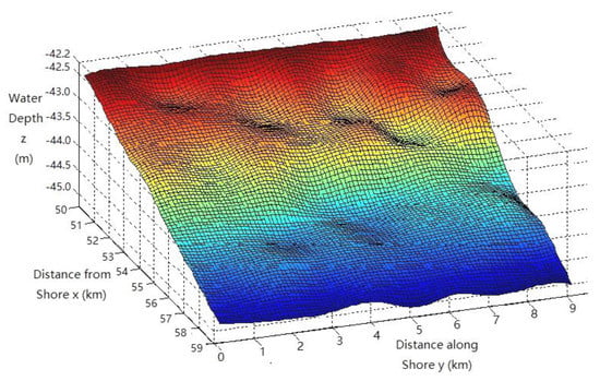
Figure 1.
3D seabed model.
2.3. Coordinate System
Taking into account that the OWF layout pattern was a circle and the water depth varied in the vertical direction, the model of the OWF was built in a cylindrical coordinate system for analysis. As delineated in Figure 2, the location of the offshore substation (OS-S) was set to be the origin, and each WT’s coordinate is denoted as . The axial distance is the Euclidean distance from the z-axis to the point . The azimuth is the angle between the reference direction on the reference plane and the line from the origin to the projection of on that plane. The axial coordinate is the vertical distance from the reference plane to the point . Because the surface function of the seabed was predefined, if the and coordinates of any WT were given, the altitude coordinate of the WT could be directly obtained.
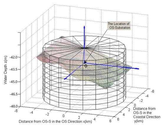
Figure 2.
OWF in the cylindrical coordinate system analysis model.
As shown in Figure 3, the projection points of two WTs on the x-o-y plane are denoted as and , respectively, where and are the distances from the origin to and and and are the angle offsets from the positive axis. Then, the distance and angle between the two points are calculated as:
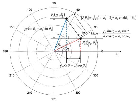
Figure 3.
Polar coordinate system analysis model.
If , that is and are on the same circumference, then (1) can be simplified to:
where is the radius of the circle where and are positioned.
If , that is and are in the same direction, then (1) and (2) can be reduced to:
In this way, the calculation of an OWF with a circular pattern can be greatly reduced.
The projection of the cylindrical coordinate system on the x-o-z (y-o-z) plane is shown in Figure 4, where the projection points of two WTs on the x-o-z (y-o-z) plane are denoted as and , respectively. The altitude difference between the two points is , and the geometric distance between the two WTs and is as follows.
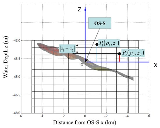
Figure 4.
Projection on the x-o-z(y-o-z) plane.
It is worth noting that the geometric distance between WTs is used for computing the wake deficit, not for calculating the inner cable length.
2.4. WT Modeling
2.4.1. WT Selection
Due to the advance of technology and the development of the wind power industry, the capacity of WTs installed in the OWFs has rocketed up from 1 MW to nearly 10 MW in recent years. Consequently, there is a wide range of WTs with different sizes for selection, which makes possible multiple types of WTs to be built in an OWF.
Theoretically, arbitrary types of WTs can be implemented in an OWF. In order to avoid the complexity of computation and analysis, this paper selects only two typical WTs that are widely used in real OWFs, namely the Vestas V164 8 MW WTs [19] and the Siemens SWT-4.0-130 4 MW WTs [20]. The parameters and power curves of those two kinds of WTs are given in Table 1 and Figure 5.

Table 1.
Parameters of the WTs.
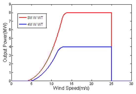
Figure 5.
Power curves of the two types of WTs.
The maximum rated capacity of the designed OWF was limited to 160 MW. Based on the span of individual WT capacity (4 MW and 8 MW), the OWF would feature from 40 to 20 WTs.
2.4.2. Wind Scenario
Generally, the wind scenario over an OWF is mainly determined by two factors: i.e., wind speed and wind direction . To model the wind scenario, a wind measurement campaign should be conducted at the OWF area where it is planned to be built to collect a large quantity of wind data. The measured data then need to be converted into the wind speed at the hub height of the WTs by (7) [12].
where denotes the wind speed measured at the height of and is the wind speed predicted at the height . is the roughness length, which is set to be 0.0001 m. stands for the natural logarithm.
As deducted in [21], the joint distribution can be modeled by a probability density function , which is derived from the Weibull distribution. It is widely used for wind speed modelling:
where is the shape parameter, is the scale parameter, and is the frequency of occurrence for each wind direction.
In this work, the joint distribution is obtained from real wind data measurement from the Horns Rev I WF [11,21], as shown in Figure 6.
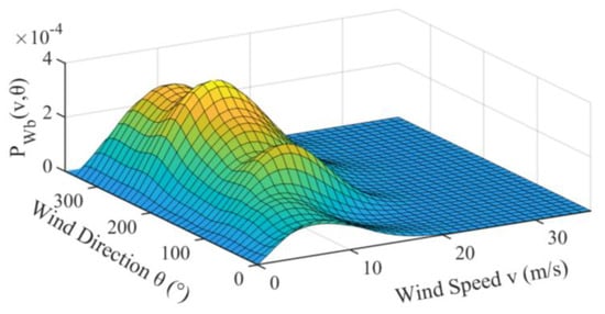
Figure 6.
PDF of wind speed and wind direction [21]. Reproduced from [21], the name of the publisher: Energies.
2.4.3. Wake Model
For a given freestream inflow condition in a polar coordinate, the wake effect between any two adjacent WTs can be firstly calculated using the Frandsen-Gaussian (F-G) wake model [11,12,22], with the basic equations as given below.
It holds for all and . is the wind speed at the distance and radius of the WT, and is the inflow wind speed. is the standard deviation of the distribution, which is termed the characteristic width. is an undetermined coefficient of . is the radius of the WT’s rotor. is the thrust coefficient. is the radius of the wake at the distance . is the actuator disk radius, and is the entrainment constant. The effective wind speed at each WT (, i.e., the effective wind speed the th WT experiences) can be evaluated. The calculation of and can be obtained from [12].
The synthesis methods of multiple WTs’ wakes include the second norm method [12,23] when WTs are in a parallel pattern and the multiplication method [12,23] when WTs are in a cascaded pattern.
2.4.4. Total Power Output of the WF
The power generated by each WT under this inflow condition can then be computed based on the power curve of each type of WT, which is shown in Figure 5. Combined with the PDF of the wind condition, the expected total power produced by the WTs at time can be written as:
where is the power curve function of the th type of WT and is the total number of the th type of WTs. is the number of total WT types.
The annual energy generation (AEP) of the whole OWF is:
where denotes the th hour in one year in which the OWF operates.
2.5. Cable Selection
2.5.1. Inner-Circle Cables
The length of the individual cables between WTs depends on the size of WTs or the configuration of the site. It was expected that the larger the WT rotor diameter was, the larger the distance was between the WTs. After pulling the cable into the J tubes on the foundation structure of the WT, the cables were fixed to a hang-off flange. At the OS-S, the cables were fixed to a cable deck. As the internal voltage of the OWF was 33 kV, the typical cable characteristics of 33 kV inner-circle cables are delineated in Table 2 [8].
Table 2.
Typical characteristics of 33 kV cables.
As pointed out in [8], the ring structure of the cable layout has higher reliability than the string structure because when one part of the cables fails in a ring, the ring is divided into two strings that can transport power separately. In this way, the operation of the whole OWF will not be affected immediately. On this account, the inner-circle/inner-array cable layout in this work is designed to have a ring structure.
Since the surface of the seabed is uneven, a geodesic algorithm [24] was implemented to find the shortest distance between any two adjacent WTs. In this way, the layout and length of the inner-circle cables can be defined.
2.5.2. Export Cable
The export cables were running from the OS-S to the onshore landing point where the distance was about 50 km. A 220 kV submarine cable extended from the OS-S to the onshore substation, which could transport at most 180 MW, in accordance with the OWF’s capacity. Since the location of the offshore and onshore substations’ coordinates were decided in advance, the export cable’s type and length were decided accordingly. In this study, the optimization of the export cable layout design was not taken into consideration.
3. OWF Optimization Model
3.1. Economic Model
The capital expenditure (CAPEX) of an OWF consists of several factors such as investment cost, O&M cost, land rent capital, and so on. To simplify the fitness function, only the investment cost of the OWF is considered and modified for mixed-installation:
where the first term is the investment cost of buying WTs. and are the costs of buying a single 8 MW WT and a single 4 MW WT, respectively. is the total number of 8 MW WTs, and is the total number of 4 MW WTs. The second term is the investment cost of the turbine foundations’ construction. is the foundation cost of the th WT, which is a function of water depth [25], as shown in Figure 7. The third term is the investment cost of the inner-circle cables in the OWF. is the cost of buying of cable of type , . is the total length of the type cable.
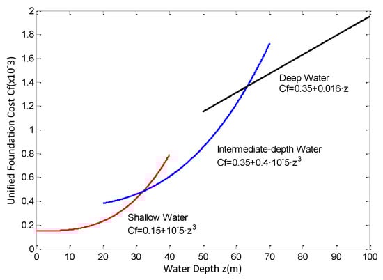
Figure 7.
Relationship between WTs’ foundation cost and water depth [12]. Reproduced from [12], the name of the publisher: IEEE.
3.2. Objective Function
The cost of energy CoE (£/MWh) (CoE = CAPEX/AEP) is the objective function, and its minimization is the objective of the optimization process. In practice, the OWF optimization problem has several constraints. The safe distance between any two WTs was set to be not less than , with being the WT rotor diameter. Besides, the WTs were not allowed to be installed beyond the OWF’s boundary. Then, the optimization problem can be formulated as follows:
where is the distance between the th WT and the th WT, which can be calculated by (6). is the minimum distance allowed between any two WTs. is the distance from the th WT to the -axis in the cylindrical coordinate system, and is the radius of the OWF’s planned circle. is the total number of WTs installed in the OWF.
3.3. Optimization Algorithm
The OWF is a very sophisticated multi-input and multi-output (MIMO) nonlinear system with time varying, strong coupling characteristics. The optimization in this case is beyond the traditional calculus based optimization algorithms. WOA [26] was utilized to solve the OWF optimization problem, which mimics the social behavior of humpback whales, i.e., the bubble-net hunting strategy. Humpback whales follow both a shrinking cycle and spiral shaped path simultaneously. There is an assumption of a 0.5 probability that the whale will choose between two mechanisms to update its positions. The general mathematical model during the optimization is shown in (16) [26].
where indicates the th iteration, is the position matrix, and is the position matrix of the best solution obtained so far. is a constant for defining the shape of the logarithmic spiral, and and are random numbers belonging to the interval . =, , and indicates the distance of the th whale to the prey (best solution obtained so far). and are coefficient vectors, which are calculated as follows [26].
where is a parameter that linearly decreases from two to zero over the course of iterations and is a random vector in .
The WOA begins with a set of random solutions. At each iteration, search agents update their positions with respect to either a randomly chosen search agent or the best solution achieved so far. The parameter decreases from two to zero in order to provide exploration and exploitation, respectively. A random search agent is chosen when , while the best solution is selected when for updating the position of the search agents. At last, the WOA is terminated by the satisfaction of a termination criterion.
The aim of the iteration of the WOA is to find the best WTs’ positions and types as the configuration for an OWF on a given terrain with a circular boundary. Each position matrix of the whales represents the parameters of the individual WT as with denoting the position of the WTs in the polar coordinate and denoting the type of WT selected in this position, e.g., if , this means the first type of WT (Vestas 8 MW) is away from the -axis and deviating from the east direction.
When iterations are carried on until the convergence criteria are satisfied, the global optimal individual is exported as the solution to the position and type selection scheme for multiple types of WTs’ mixed-installation. Eight hundred generations were set for the WOA to finish the evolution, except that the iterations reached the minimum residual set as .
4. Case Study
4.1. Baseline Cases
Among the operational OWFs, the majority are composed of an identical type of WTs arranged in symmetrical and array-like layouts. As reference cases, this paper puts forward four baseline designs with the same total capacity (160 MW), but each of them consists of different types of WTs. The first one is composed of 40 Siemens 4 MW WTs with Cb1 (Figure 8), and the second one is composed of 20 Vestas 8 MW WTs with Cb2 (Figure 9), occupying the same area (a circle with a radius of 2500 m). For comparison, the layouts of an OWF that has the same total capacity, but occupies a rectangle area with a size 5166 m by 4018 m are shown in Figure 10; Figure 11, respectively. The layout and spacing between WTs were in the similar manner as in Horns Rev 1 WF [21].
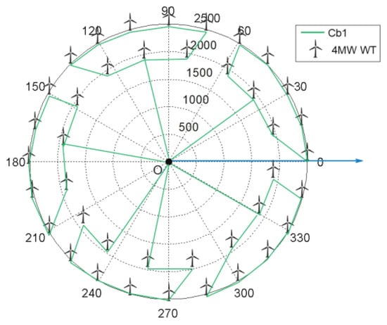
Figure 8.
Baseline 1.
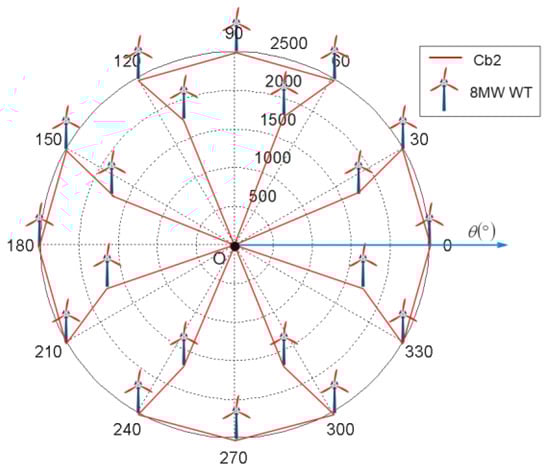
Figure 9.
Baseline 2.
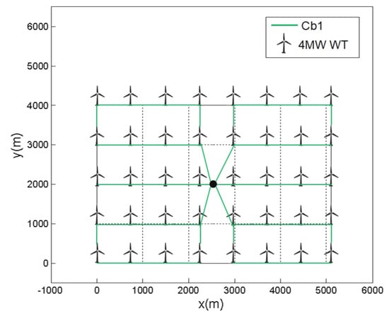
Figure 10.
Baseline 3.
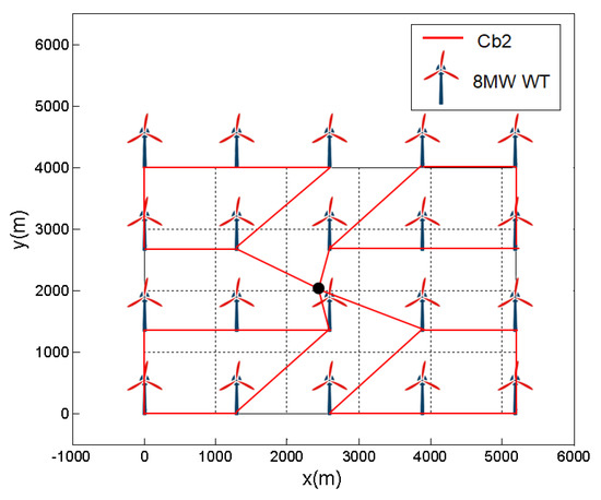
Figure 11.
Baseline 4.
Table 3 shows the calculation results of the four baselines (BL1–BL4). The definition of the parameters is described below.
Table 3.
Comparison of Baselines (BLs) 1–4.
Power density is the power generated by the OWF per unit area () and is calculated as follows:
where is the OWF planning area.
The efficiency is calculated as in (20).
where is computed using (12), and the denominator is the ideal expected total power, which is the power production if there are no wake effects. is the ideal expected output power of the th WT at time , and is the total number of WTs.
The capacity factor (CF) is computed as in (21).
where is the rated power of the th WT.
From Table 3, the following conclusions can be drawn.
Firstly, the OWF in a circular layout outperformed that in a rectangle layout because the circular layout occupied a smaller area and the radial distance between WTs was much longer than the distance between adjacent WTs in an array. This could reduce the interaction between WTs and consequently decrease wake loss. Besides, the total length of cables was considerably shorter in the circular layout, which helped reduce the ohmic losses in the cables.
Secondly, WTs with larger capacity would help improve the OWF’s energy efficiency. For the design with larger WTs, the hub heights were higher; thus, the wind resource was better; the number of WTs required was fewer, and the spacing was larger in terms of rotor diameters; thus, the wake effect was weaker (also suggested by the higher OWF efficiency).
Lastly, it was not economic to implement larger WTs compared with smaller ones, since the upscaled dramatically with the increase of WTs’ capacity. As the capital cost per MW increased with WT size, the baseline designs with smaller WTs were better from an economic angle.
Generally, the above comparisons demonstrated that: (i) a circular layout plan is much better than a rectangle layout plan for the OWF; (ii) from the efficiency and economic perspective, different types of WTs have their different competitive strengths, respectively. These points clearly suggest that it would be beneficial to investigate the mixed installation of WTs in a circular layout pattern.
4.2. Optimized Cases
For comparison, this paper first gives the optimized design (OD1 and OD2) of BL1 and BL2, comprised of uniform WTs. The simulation results are shown in Figure 12 and Figure 13, respectively. The optimization result of the OWF with mixed-installation of WTs is shown in Figure 14.
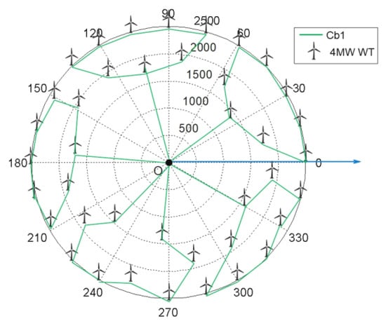
Figure 12.
Optimized Design 1.
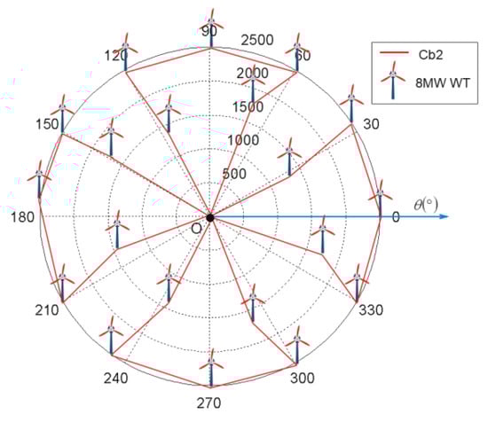
Figure 13.
Optimized Design 2.
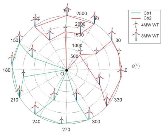
Figure 14.
Optimized Design 3.
Table 4 shows the simulation results and comparisons between OD1 to OD3 and BL1 and BL2. Based on these results, it can be clearly seen that the optimized designs (OD1 to OD3) generally exceeded the baseline cases (BL1 and BL2) in terms of energy production (AEP, CF, wake deficit, and cable ohmic losses) and economy (). This conclusion was in accordance with previous research [10]. This also justified the effectiveness of the WOA to find the optimal solution.
Table 4.
Comparison of Optimized Designs (OD) 1–3 and Baselines 1, and 2.
For given wind conditions, five main factors strongly affected the simulation results: (1) wake deficit, (2) cable ohmic losses, (3) capital cost of different types of WTs, (4) capital cost of different types of cables, and (5) foundation cost of WTs installed in different water depth areas. (1) and (2) were from the electricity output aspect, while (3), (4), and (5) were from the capital investment aspect. 8 MW WTs had stronger electricity generation ability and could save more space in the case of a given capacity. Nevertheless, the mean capital cost of 8 MW WTs was usually higher than that of 4 MW WTs. In addition, Cb1 was less expensive than Cb2, but its transmission capacity was lower and its resistance higher. Thus, the merits of the non-uniform design were quite dependent on the proportion that different WTs occupied and the cable types. However, its possible demerits in terms of supply chain management, installation, and O&M distinctly appeared on account of the inevitably increased level of complexity for these concerns.
5. Conclusions
This paper proposed a novel optimization framework involving mixed-installation for OWF with a circular boundary. Two kinds of WTs with different rated capacities, diameters, hub heights, and power curves were considered for micro-siting in a deep water OWF. A complete optimization problem was established including wind profile, water depth, wake effects, space constraints, and cable layout. The WOA optimization method was implemented to solve the WTs’ positioning problem with different capacity mixing ratios of the two types of WTs. Extensive simulation work was presented to validate that the proposed scheme could give the best layout result of the optimization object.
The method developed in this study is a useful tool for OWF design. It benefits the designers to further explore the feasible design space for OWFs and acquire even lower by considering non-uniform design options using multiple types of WTs. Further research can include three aspects: (i) the improvement of the algorithm efficiency and the complex constraints including different safe distances for different WTs; (ii) the refinement of the optimization model by taking other relative factors into consideration; (iii) the performance comparison of the WOA and other optimization algorithms to solve the WF optimization problem should be taken into consideration. Besides, more efficient algorithms should be developed to address this problem.
Author Contributions
Conceptualization, S.T.; methodology, S.T.; software, S.T.; validation, S.T., J.Z. and G.Z.; formal analysis, A.F.; investigation, A.F.; resources, S.T.; data curation, J.Z.; writing, original draft preparation, S.T.; writing, review and editing, A.F.; visualization, S.T.; supervision, G.Z.; project administration, G.Z.; funding acquisition, G.Z. All authors have read and agreed to the published version of the manuscript.
Funding
This work is supported by the “Excellence Project Funds of Southeast University” and the National Natural Science Foundation of China (Grant Nos. 81671667, 81471644, and 81101039 to G.Z.).
Conflicts of Interest
The authors declare no conflict of interest.
Nomenclature
| Abbreviation | |
| OWF | offshore wind farm |
| WT | wind turbine |
| WOA | wale optimization algorithm |
| GA | genetic algorithm |
| PSO | particle swarm optimization |
| AI | artificial intelligence |
| O&M | operation and maintenance |
| CoE | cost of energy |
| WF | wind farm |
| OS-S | offshore substation |
| AEP | annual energy production |
| CAPEX | capital expenditure |
| OD | optimized design |
| BL | baseline |
| MIMO | multi-input and multi-output |
| CF | capacity factor |
| F-G | Frandsen-Gaussian |
| Notation | |||
| Euclidean distance from the -axis to the point in the cylindrical coordinate system | angle offset from the positive -axis in the cylindrical coordinate system | ||
| vertical distance from the reference plane to the point in the cylindrical coordinate system | wind speed measured at the reference height | ||
| reference height where wind speed is measured | roughness length | ||
| Weibull distribution | shape parameter of Weibull distribution | ||
| scale parameter of the Weibull distribution | frequency of occurrence in each wind direction | ||
| an undetermined coefficient of in the F-G model | WT thrust coefficient | ||
| WT rotor radius | WT entrainment constant | ||
| number of total WT types. | WT total number | ||
| minimum distance allowed between any two WTs | WF covered area | ||
| WF power density | WF efficiency | ||
References
- Millais, C.; Teske, S. Wind Force 12-a Blueprint to Achieve 12% of the World’s Electricity by 2020; European Wind Energy Association and Greenpeace: Brussels, Belgium; Hamburg, Germany, 2003. [Google Scholar]
- Prabhu, N.P.; Yadav, P.; Prasad, B.; Panda, S.K. Optimal placement of off-shore wind turbines and subsequent micro-siting using Intelligently Tuned Harmony Search algorithm. In Proceedings of the IEEE Power Energy Society General Meeting, Vancouver, BC, Canada, 21–25 July 2013. [Google Scholar]
- Mosetti, G.; Poloni, C.; Diviacco, B. Optimization of wind turbine positioning on large wind farms by means of a genetic algorithm. J. Wind Eng. Ind. Aerodyn. 1994, 51, 105–116. [Google Scholar] [CrossRef]
- Grady, S.A.; Hussaini, M.Y.; Abdullah, M.M. Placement of wind turbines using genetic algorithms. Renew. Energy 2005, 30, 259–270. [Google Scholar] [CrossRef]
- Parade, L.; Herrera, C.; Flores, P.; Parada, V. Assessing the energy benefit of using a wind turbine micro-siting model. Renew. Energy 2018, 11, 591–601. [Google Scholar] [CrossRef]
- Xie, K.G.; Yang, H.J.; Hu, B.; Li, C.Y. Optimal layout of a wind farm considering multiple wind directions. In Proceedings of the International Conference on Probabilistic Methods Applied to Power Systems (PMAPS), Durham, UK, 7–10 July 2014; pp. 1–6. [Google Scholar]
- Kuo, J.Y.; Romero, D.A.; Beck, J.C.; Amon, C.H. Wind farm layout optimization on complex terrains-integrating a CFD wake model with mixed-integer programming. Appl. Energy 2016, 178, 404–414. [Google Scholar] [CrossRef]
- Gong, X.; Kuenzel, S.; Pal, B.C. Optimal wind farm cabling. IEEE Trans. Sustain. Energy 2018, 9, 1126–1136. [Google Scholar] [CrossRef]
- Fischetti, M.; Pisinger, D. Optimizing wind farm cable routing considering power losses. Europ. J. Oper. Res. 2018, 270, 917–930. [Google Scholar] [CrossRef]
- Feng, J.; Shen, W.Z. Design optimization of offshore wind farms with multiple types of wind turbines. Appl. Energy 2017, 205, 1283–1297. [Google Scholar] [CrossRef]
- Tao, S.Y.; Xu, Q.S.; Feijóo, A.; Hou, P.; Zheng, G. Bi-hierarchy optimization of a wind farm considering environmental impact. IEEE Trans. Sustain. Energy 2020, in press. [Google Scholar] [CrossRef]
- Tao, S.Y.; Kuenzel, S.; Xu, Q.S.; Chen, Z. Optimal micro-siting of wind turbines in an offshore wind farm uisng Frandsen-Gaussian wake model. IEEE Trans. Power Syst. 2019, 34, 4944–4954. [Google Scholar] [CrossRef]
- Wilson, D.; Rodrigues, S.; Segura, C.; Loshchilove, I.; Huttere, F.; Buenfil, G.L.; Kheiri, A.; Keedwell, E.; Ocampo-Pineda, M.; Özcanh, E.; et al. Evolutionary computation for wind farm layout optimization. Renew. Energy 2018, 126, 681–691. [Google Scholar] [CrossRef]
- Wu, Y.K.; Lee, C.Y.; Chen, C.R.; Hsu, K.W.; Tseng, H.T. Optimization of the wind turbine layout and transmission system planning for a large-scale offshore wind farm by AI technology. IEEE Trans. Ind. Appl. 2014, 50, 2071–2080. [Google Scholar] [CrossRef]
- Song, M.X.; Chen, K.; Wang, J. Three-dimensional wind turbine positioning using Gaussian particle swarm optimization with differential evolution. J. Wind Eng. Ind. Aerodyn. 2018, 172, 317–324. [Google Scholar] [CrossRef]
- Kazari, H.; Oraee, H.; Pal, B.C. Assessing the effect of wind farm layout on energy storage requirement for power fluctuation mitigation. IEEE Trans. Sustain. Energy 2019, 10, 558–568. [Google Scholar] [CrossRef]
- Tang, X.Y.; Shen, Y.; Li, S.L.; Yang, Q.M.; Sun, Y.X. Mixed installation to optimize the position and type selection of turbines for wind farms. In Proceedings of the Neural Information Proceedings: 24th International Conference, Guangzhou, China, 2017, 14–18 November 2017; Part VI. pp. 307–315. [Google Scholar]
- Rodrigues, S.; Restrepo, C.; Katsouris, G.; Pinto, R.T.; Soleimanzadeh, M.; Bosman, P.; Bauer, P. A multi-objective framework for offshore wind farm layouts and electric infrastructures. Energies 2016, 9, 216. [Google Scholar] [CrossRef]
- Vestas V164-8MW. Available online: https://en.wikipedia.org/wiki/Vestas_V164 (accessed on 1 January 2020).
- Siemens 140 SWT-4.0-130 4MW. Available online: https://en.wind-turbine-models.com/turbines/601-siemens-swt-4.0-130 (accessed on 1 January 2020).
- Feng, J.; Shen, W.Z. Modelling wind for wind farm layout optimization using joint distribution of wind speed and wind direction. Energies 2015, 8, 3075–3092. [Google Scholar] [CrossRef]
- Bastankhah, M.; Porte-Agel, F. A new analytical model for wind turbine wakes. Renew. Energy 2014, 70, 116–123. [Google Scholar] [CrossRef]
- Jensen, N.O. A Note on Wind Generator Interaction; Risø-M-2411; Risø National Laboratory: Roskilde, Denmark, November 1983. [Google Scholar]
- Kirsanov, D. November 2017. Available online: http://www.mathworks.com/matlabcentral/fileexchange/18168-exact-geodesic-for-triangular-meshes (accessed on 1 January 2020).
- González, J.S.; Payán, M.B.; Santos, J.R. A new and efficient method for optimal design of large offshore wind power plants. IEEE Trans. Power Syst. 2013, 28, 3075–3084. [Google Scholar] [CrossRef]
- Mirjalili, S.; Lewis, A. The whale optimization algorithm. Adv. Eng. Soft. 2016, 95, 51–67. [Google Scholar] [CrossRef]
© 2020 by the authors. Licensee MDPI, Basel, Switzerland. This article is an open access article distributed under the terms and conditions of the Creative Commons Attribution (CC BY) license (http://creativecommons.org/licenses/by/4.0/).