1. Introduction
Modern battery management systems (BMSs), among other functionalities, include a number of algorithms for estimating key battery state variables such as state-of-charge (SoC) and remaining available charge capacity, and model parameters such as internal resistance [
1]. The SoC estimate can be used for predicting the current vehicle range, as well as for identification of current battery operating point which is important from the standpoint of ensuring battery safety. On the other hand, the internal resistance and capacity estimates are the main indicators used for tracking the battery degradation level, i.e., estimation of battery state-of-health (SoH) [
2]. Furthermore, almost every battery model parameter is changing with battery degradation, so that for robust SoC and SoH estimation, those changes should be accurately tracked, as well.
Battery state and parameter estimation algorithms are often based on Kalman filters (KF), which in its basic linear version represent an optimal recursive solution for estimating hidden states of a linear, time-varying Gaussian system (i.e., probabilistic inference) [
3]. While the Gaussian assumption holds in many cases based on the central limit theorem, the battery model is inherently nonlinear, which calls for application of nonlinear KF forms. Two of the most widely used nonlinear KFs are extended Kalman filter (EKF) and sigma-point Kalman filter (SPKF) [
3]. The EKF relies on analytical linearization of the model around a time-varying operating point (i.e., an expected value of the estimated random state), while SPKF statistically linearizes the model around several operating points (depending on the number of states that are estimated).
Topic of state and parameter estimation of Li-ion battery cells has been addressed by many previous studies. One of the first implementations of dual extended Kalman filter-based (DEKF) estimator of SoC and resistance parameters can be found in [
4]. Researchers have been upgrading the estimators ever since, e.g., using an adaptation mechanism for process noise variance recalculation [
5], or applying more advanced filters such as SPKF [
6] or particle filter (PF) [
7]. These approaches are based on the assumption of constant model parameters/characteristics such as the SoC-dependent open-circuit voltage (OCV) characteristic
or battery remaining capacity. Since those parameters are in fact dependent on SoH [
8] and temperature [
9], they should be estimated as well, for accurate and robust overall estimation.
There are several studies that account for
variation with SoH by implementing the offline identified response surface model of
with respect to SoC and remaining capacity [
10,
11,
12]. Authors in [
13] use the model migration method to adapt an offline trained model. An obvious disadvantage of this approach is related to the need of having a large data set from previously conducted aging experiments on the same cell type, as well as lack of temperature dependency in the response surface model. This disadvantage is tackled in this paper by describing the characteristic
with a model whose parameters are estimated along the rest of model states and parameters within the DEKF structure. Moreover, this approach includes an adaptation mechanism of
which allows for identification of
hysteresis profile.
Remaining capacity estimators based on EKF and PF can be found in [
14], while a recursive approximate least-squares approach is proposed in [
15]. In both cases the characteristic
is again considered as a constant-parameter dependence. Dual estimation of SoC and capacity can be found in [
16], where authors use multiscale estimation with the online identified model, which can be regarded as a next step towards complete estimator. Certain weaknesses of that approach include: (i) Still an offline identified
map is used, (ii) capacity estimate shows considerable variations in steady state, and (iii) the capacity estimator needs to be turned on manually after 25 min in order to ensure overall estimator stability. The multiscale estimator presented in this paper improves the capacity estimation accuracy and flexibility by using a more accurate SPKF and automated turning on the capacity estimator by means of applying a convergence detection algorithm.
Finally, a fully-electric scooter-based experimental verification of the proposed battery estimators is conducted, including consideration of different temperature operating points.
2. Experimental Setup
The experimental setup includes the fully-electric scooter Govecs S2.6+, powered by the 3.3 kW BLDC electric motor and the battery pack of 400 Li-Ni
0.33Mn
0.33Co
0.33O
2 (Li-NMC) cells, connected in the 20 × 20 matrix [
17], with the total nominal voltage of 72 V, and the total energy capacity of 4.1 kWh. Battery pack is equipped with BMS which provides basic battery measurements and estimates accessible through the scooter CAN bus.
Electric scooters became an attractive transportation solution in urban areas with mild climate conditions, thus contributing to the current transport electrification effort aimed at reducing traffic congestion, and air and noise pollution. There are already several strong electric scooter manufacturers in the EU (and worldwide), e.g., Govecs, Ujet, Hrowin, Torrot, etc. NMC-type Li-ion batteries represent a preferred energy storage solution in scooter applications [
17], because they offer favorable energy density, while not experiencing high loads (in terms of battery C-rate) and not operating in extreme, particularly low temperature conditions, in those applications.
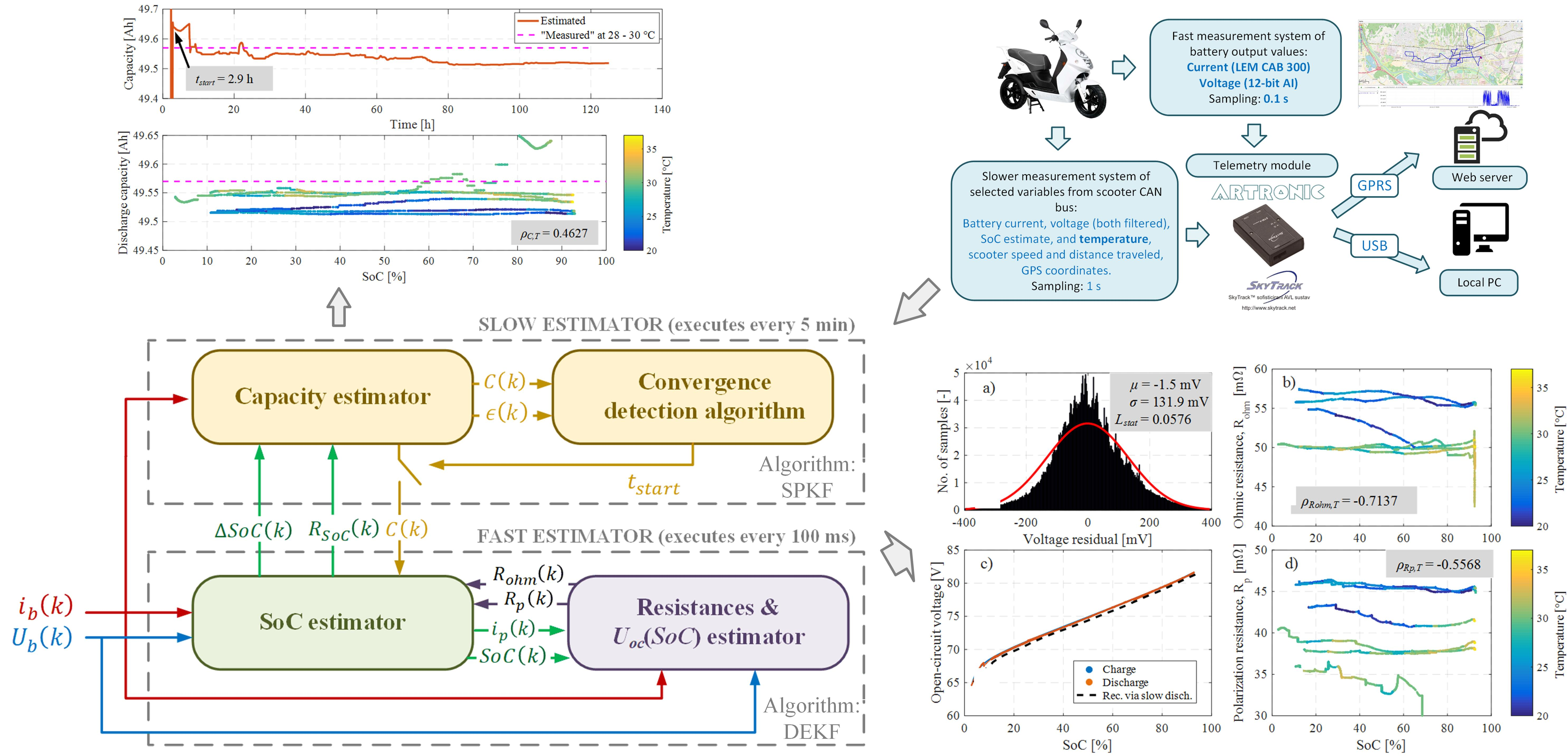
For the research purposes, the scooter has been equipped with the measurement and telemetry system illustrated in
Figure 1. The system is built around the Artronic SkyTrack telemetry module, custom-programmed for the acquisition and storage of measurement data, as well as for communication with the server through GPRS connection in real time. The measurement system consists of voltage and current measurement on battery output nodes, and acquisition of data available from the scooter CAN bus. The battery current is measured by using a precise, low-offset current transducer (LEM CAB 300, [
18]), while the battery voltage is measured through a 12-bit analogue input of the telemetry module. Those two measurement values are sampled every 0.1 s and stored in the module. Selected values from the scooter internal CAN bus, such as battery voltage, current and temperature, vehicle’s distance travelled, motor on/off flag, as well as the vehicle’s current GPS coordinates and longitudinal velocity are stored with the sample rate of 1 s. GPRS connection is used to send data relevant for real-time tracking of scooter, such as its GPS coordinates, battery SoC, and other diagnostic parameters. The whole measurement dataset, including the fast current and voltage measurements, is stored in the telemetry module memory card and can be occasionally downloaded through USB connection to a local PC.
3. Battery Pack Model
This section first presents a battery mathematical model used as a basis for SoC estimator design. Next, models employed for estimation of battery internal parameters used by the SoC estimator are presented. Finally, two offline identification experiments are described, which have been conducted to determine battery model parameters that are considered as constant or used in estimator verification.
3.1. Mathematical Model
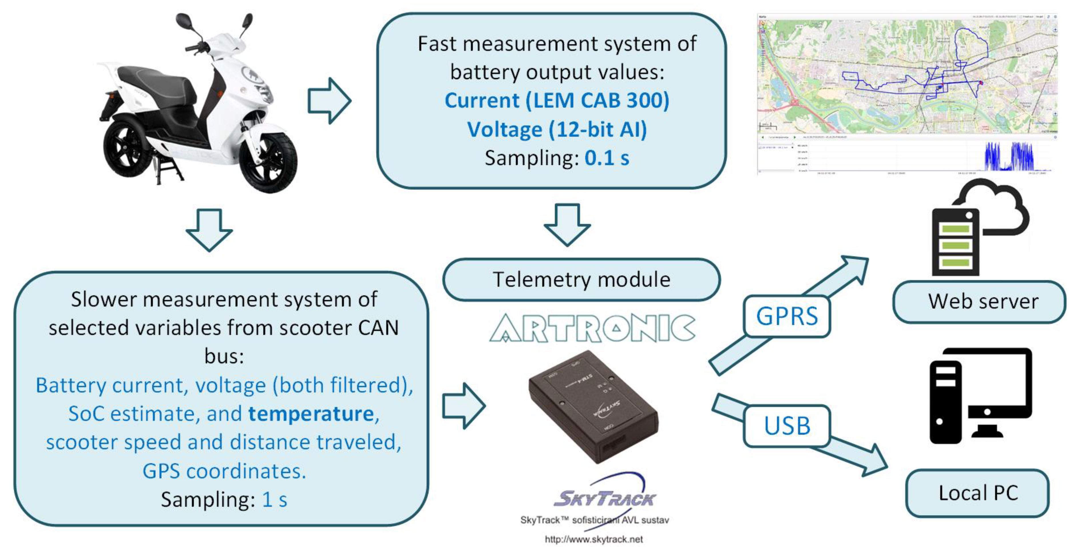
The battery model used in this research is based on the equivalent-circuit model (ECM) showed in
Figure 2, which consists of (i) a voltage source dependent on the battery SoC, i.e., the OCV characteristic
, (ii) an ohmic resistance
which models voltage drops in the electrolyte and electrical contacts, and (iii) a single polarization RC term (
and
) which models the slow battery dynamics, i.e., diffusion process. It should be noted that the diffusion process is more accurately modelled with the Warburg element [
19] which is here avoided due to the complexity, but it can be approximated by a single or more RC elements connected in series (a single RC element is usually used as a good trade-off between simplicity and accuracy [
20]). Moreover, note that the polarization resistance
in
Figure 2 models all voltage drops that are not related to the ohmic one, including that related to charge transfer.
The above ECM can be described by the following discrete-time time-varying state-space mathematical model [
4]:
where
is the filter sampling time,
is the battery capacity,
is the polarization term time constant, and
is discrete sample step.
3.2. OCV Model
Since the battery OCV is a nonlinear function of SoC, and to a lower extent temperature [
9] and SoH [
8], it is desirable to describe it using a parametric model such as the one used in [
4]:
where vector
contains
-model parameters that need to be estimated.
3.3. Model of Internal Resistance Parameters
The presented ECM has two resistance parameters in its model. Both of those resistances are known to depend on SoH and temperature [
21]. So, it is important to have them estimated along with the model states. Since there is no resistance model feasible for online estimator implementation, resistances are modelled as random-walk variables:
where
is the identity matrix, and
is the vector containing variances of both resistances. Other variable model parameters, such as those from Equation (3), can be modelled using this approach, as well.
3.4. Identification Experiments
The battery model parameters that are assumed to be constant or used in estimator verification should be determined by means of specific (targeted) offline identification tests.
3.4.1. Battery OCV Curve
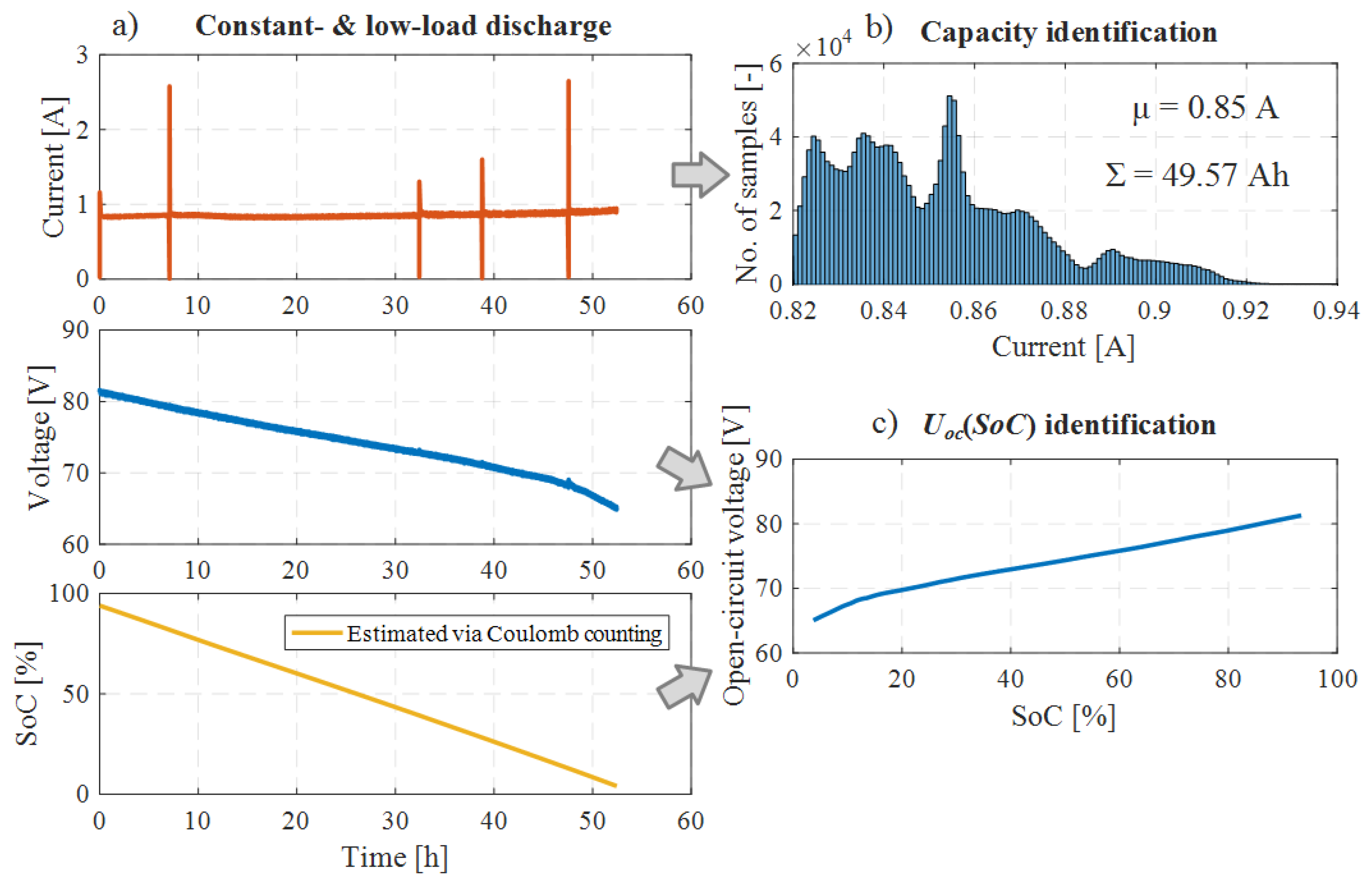
The curve
has been identified during low- and constant-load experiments (during which the vehicle was in rest, while only considerable battery load was scooter headlight), in which case any voltage drop in the battery can be neglected due to the low current (~
), so that the measured voltage
can be taken as the OCV
. The SoC was estimated by Coulomb counting, i.e., by integrating the measured current. The battery capacity was also identified in this experiment by integration of measured current during the process of full battery discharge, which gave
Ah. Graphical illustration of the identification experiment and related results are shown in
Figure 3. The identified curve
has been used in validation of
estimation results (see next sections).
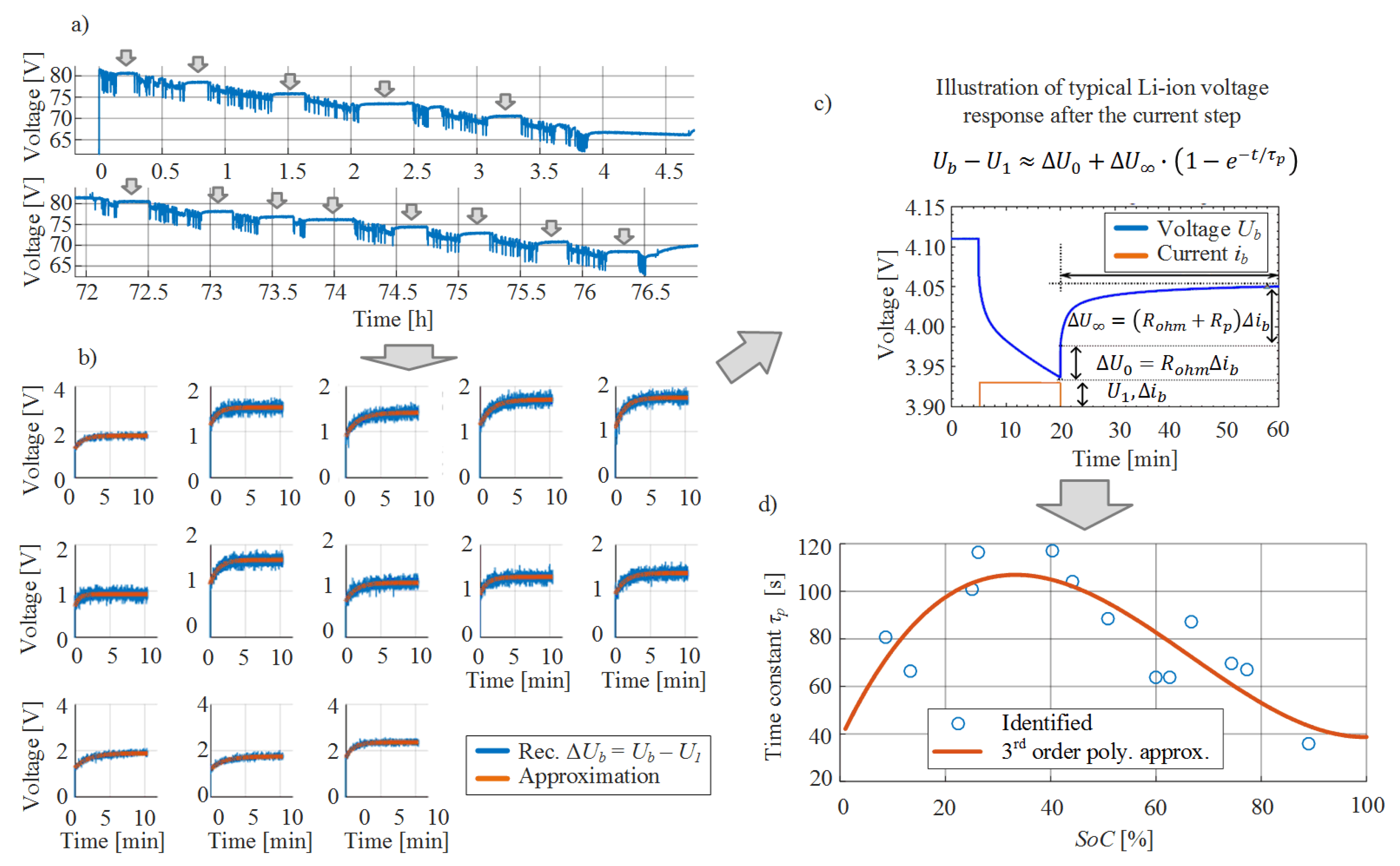
Polarization Time Constant
This parameter can be identified during the battery relaxation periods, i.e., parts of driving cycle where current has dropped to zero and remained equal to zero for at least 15 min. The relaxation transients to be identified were extracted from the voltage response (see
Figure 4a,b) and approximated with the ECM model shown in
Figure 4c.
The identified values of relaxation time constant
are shown in
Figure 4d. These values were then approximated with a 3rd-order polynomial in dependence on SoC, and that polynomial was later used for calculation of
at every estimator step based on the current, slowly changing SoC working point.
It is important to note that the polarization time constant can also vary with battery temperature and aging [
22,
23]. These effects are neglected in the estimator problem formulation in this paper, i.e., parameters of the characteristic
are not estimated online. This is motivated by the following main reasons: (i)
is not directly involved in the ECM voltage equation (see Equation (2)), thus making it weakly observable in the proposed estimator design; ii) error in
will cause an error in voltage modelling during the transient periods (i.e., before voltage has relaxed), so that the polarization dynamics may influence estimator accuracy only in transient conditions. As needed, the slow temperature- and aging-influenced polarization dynamics can be accounted for in the estimator design either by extending the
characteristic with the temperature and SOH inputs or by considering
as an additional parameter to be estimated, which is a subject of future work.
4. State and Parameter Estimator
This section deals with design, parametrization, and verification of the SoC estimator. It is designed as a dual state and parameter estimator, thus allowing for accompanying estimation of selected ECM parameters (i.e., the battery internal resistances and OCV parameters). A special attention is devoted to estimation of battery OCV hysteresis based on two complementary approaches (adapting the OCV parameters to current sign change or using an explicit hysteresis model).
4.1. DEKF-Based State and Parameter Estimator
States and parameters of the ECM are estimated with the DEKF, as a well-known approach in the model-based estimation problems where model states and slowly varying model parameters are to be estimated simultaneously [
1]. The DEKF equations are not listed here due to paper size constraints, and they can be found in [
24]. DEKF consists of two filters operating in parallel based on the state and parameter models:
| State estimator state-space model: | Parameter estimator state-space model: |
| |
| |
where
and
are the vectors of model states and inputs, respectively,
is the vector of state variances (with the corresponding covariance matrix
),
is the vector of model parameters with their variances contained in vector
(with the corresponding covariance matrix
),
is the model output function (the same output function is used in both state and parameter models),
is the measured model output vector with measurement noise and corresponding covariance matrix denoted by
and
, respectively. The complete, discrete-time state-space model for simultaneous state and parameter estimation then reads (cf. Equations (1)–(4)):
The state estimator model, given by Equations (6) and (8), is considered linear in state equation under the assumption that the nonlinearity of function can be neglected. The only nonlinearity resides in the output equation of the state estimator, related to the term (see Equation (3)), so that an EKF is finally used as a model state estimator. On the other hand, the parameter estimator model, given by Equations (7) and (8), is linear, so that the estimator reduces to KF.
4.2. Estimator Parametrization
The DEKF needs to be properly parametrized. For instance, appropriate statistic parameters such as process and output noise covariances and should be determined offline. Polarization time-constant was assumed to be degradation-invariant and used as the identified SoC-dependent profile (see previous section), while battery capacity was in this case taken as a constant value that was measured as described in the previous section. This section also describes an estimator adaptation mechanism that indirectly compensates for the influence of unmodelled hysteresis of curve .
4.2.1. DEKF Covariance Matrices Parametrization
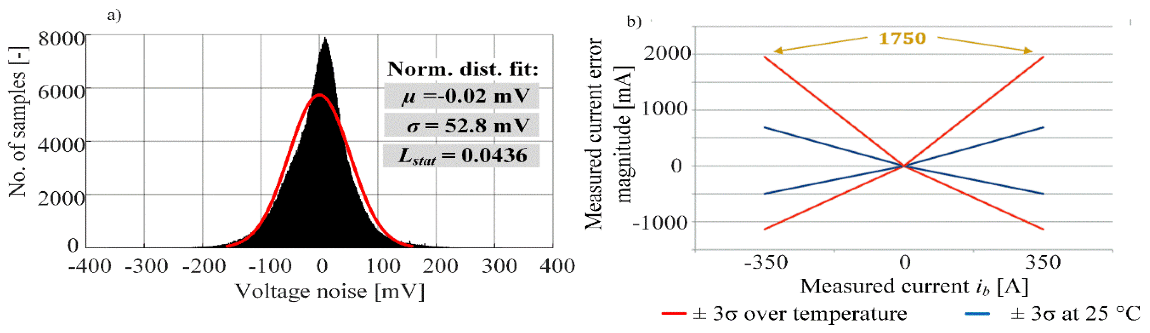
The measurement variable in the DEKF model is the battery output voltage
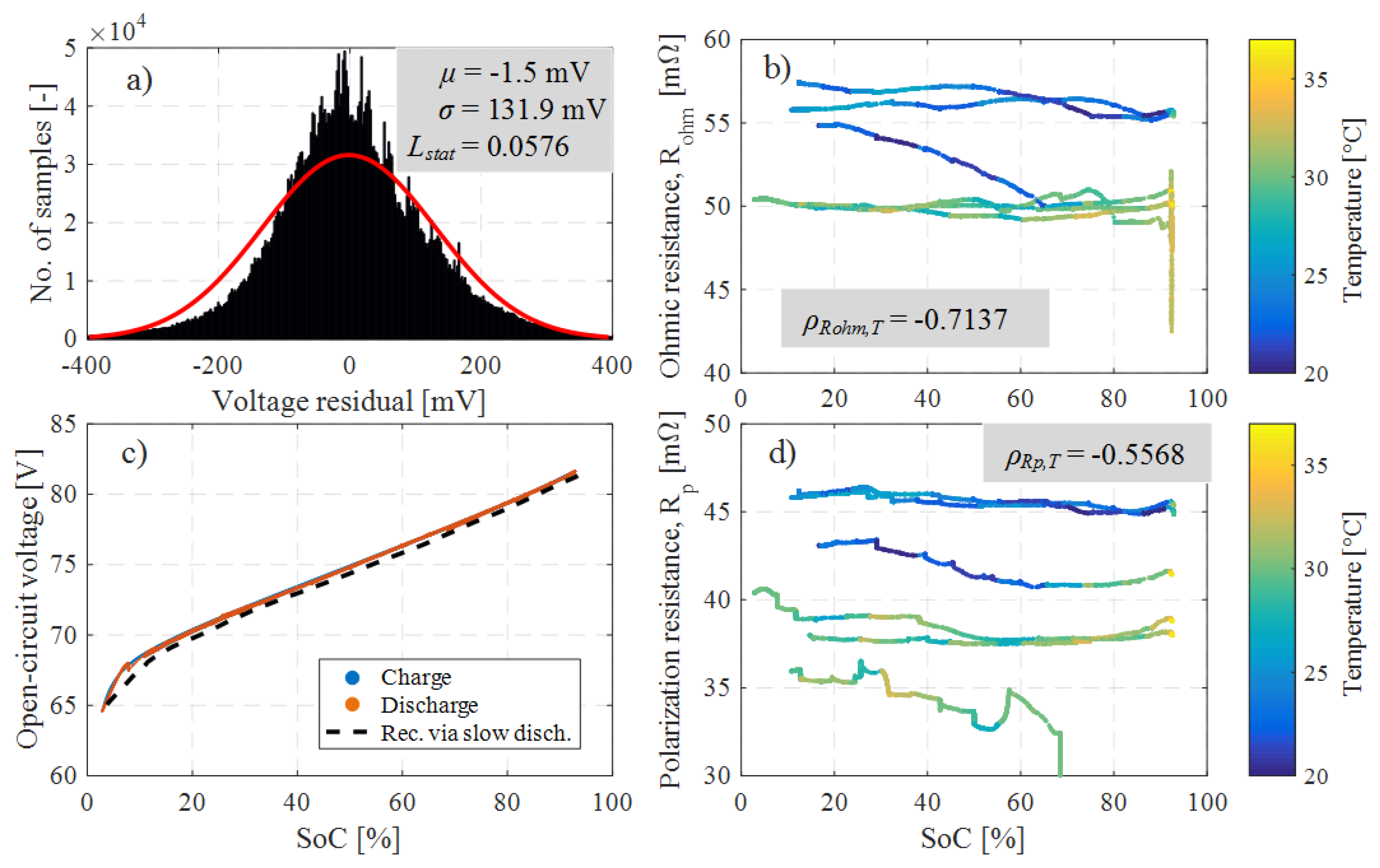
(see Equation (8)). Its measurement noise has been estimated by approximating the voltage measurement error histogram with normal distribution, as shown in
Figure 5a. The parameter
identified in
Figure 5a is the voltage noise mean value (expectation), while
is the standard deviation which, after being squared, yields the measurement covariance
mV
2. The parameter
in
Figure 5a is the result of Lilliefors normality test. Further in this paper, we calculate
for estimator voltage residuals and compare it to the calculated
of voltage sensor noise (see
Figure 5a) to check how similar they are, i.e., how accurate is the estimator.
The process noise relates to the current sensor noise, as can be seen from Equation (6). The current is in this case measured with LEM CAB 300 sensor, whose datasheet specifies a linear relation between measured current and magnitude of its measurement error (see
Figure 5b). The standard deviation of current sensor noise can be estimated as a value three times lower than the noise magnitude, and covariance matrix is then the diagonal matrix of current sensor noise variances:
4.2.2. Adaptation Mechanism
The relatively simple battery model given by Equations (1) and (2) does not take into account some secondary, but generally influential effect such as the hysteresis of OCV curve
[
25]. Since the hysteresis cannot be directly measured in this case, an adaptation mechanism is introduced in the form of single-step increase of the elements of parameter covariance submatrix
when the start or end of charging is detected. This approach allows faster convergence of the
parameters (written in
), which abruptly change when the sign of battery current (or SoC derivative) occurs due to the existence of hysteresis of
curve. Note that the battery current for the given scooter changes its sign only when the scooter is exposed to change from normal driving to charging or vice versa, because it does not incorporate regenerative braking.
4.3. Estimation Results
The presented DEKF was validated based on the recorded scooter real city driving cycle data consisting of seven load cycles (i.e., charge/discharge cycles) lasting for 150 h in total. The obtained estimation results are shown in
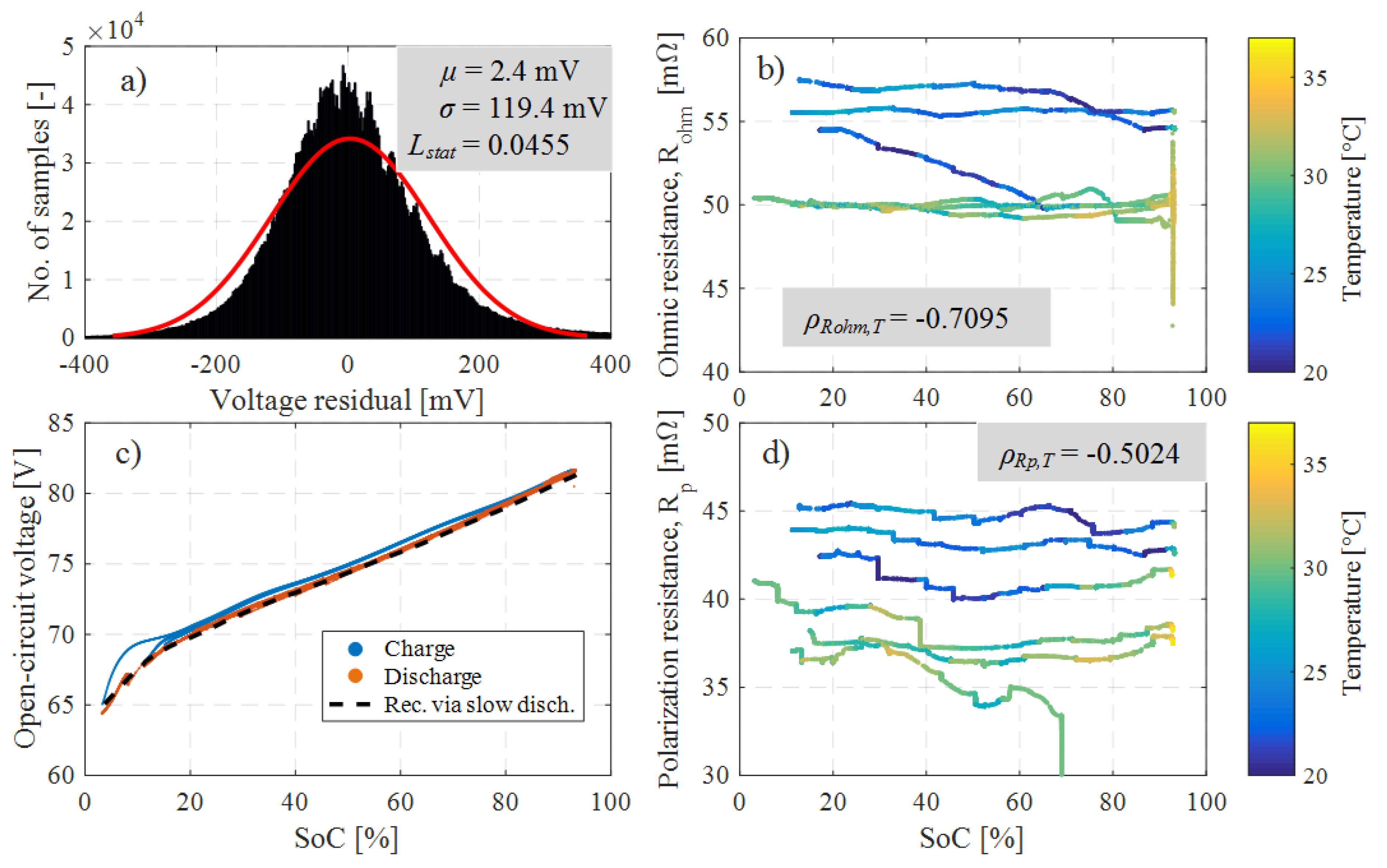
Figure 6. Since the battery SoC cannot be measured, and there is no fully reliable SoC estimate available, the DEKF accuracy is evaluated by analyzing
a posteriori voltage residual, i.e., difference between the recorded voltage
and the voltage calculated from output Equation (8) using
a posteriori estimated states and parameters. The perfectly accurate filter would reduce the voltage residual to the voltage sensor noise, i.e., the residual mean value, standard deviation, and
would be close to the values from
Figure 5a.
Figure 6a shows the voltage residuals histogram including the corresponding normal distribution fit and its parameters. Residual mean value is low, while standard deviation and
are larger than those of the voltage sensor noise. The estimated values of resistances
and
are shown in
Figure 6b,d, respectively, vs. SoC and color-mapped with respect to battery temperature. These results point out that both resistances show negative correlation with respect to temperature (note:
stands for correlation coefficient between vectors
and
, and are obtained by using the MATLAB function
corrcoef), which is expected for the Li-ion cell resistances [
21]. As of the correlation with respect to SoC (based on visual inspection of
Figure 6b,d), both
and
do not seem to be correlated with SoC, which is an expected result for the particular SoC range, based on the estimator results from the available literature [
16,
21,
26] in which resistances more significantly depend on SoC only at the very low and very large SoC bands. The estimated
curves during charging and discharging intervals are shown in
Figure 6c, along with the “measured” one adopted from
Figure 3c. Evidently, the estimated and “measured” curves are in good agreement, and a relatively small hysteresis is apparent (i.e., the charging and discharging curves do not overlap).
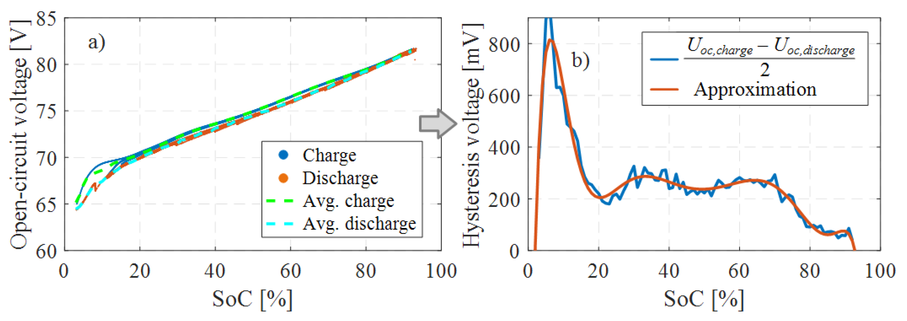
The two sets of estimated
curves from
Figure 6c have been averaged and shown as dotted lines in
Figure 7a. Half of the difference between those two curves yields the estimate of battery hysteresis voltage which is shown in
Figure 7b. The estimated hysteresis voltage trend is in line with the results from the literature (e.g., [
25]), except in the low-SoC region (
), where the estimated hysteresis is larger than what would be expected based on the literature.
Now, when the hysteresis voltage is known, the adaptation mechanism may be omitted, and the hysteresis can be accounted for directly through a proper
model extension. A complex, dynamic hysteresis model [
27] is not necessary in this case, because the particular scooter does not support regenerative breaking (i.e., its battery is not exposed to often changes of current sign). A simple, instantaneous hysteresis model can be described by introducing an auxiliary variable
described as [
4]:
(where
is the current sensor noise amplitude calculated using the current sensor variance from Equation (9)) and using it to modify the output equation (cf. Equation (8)):
where
is the hysteresis voltage value obtained from data shown in
Figure 7b by means of 10th-order approximation polynomial. Described hysteresis is used instead of the adaptation mechanism in the rest of the paper.
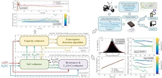
5. Battery Capacity Estimation
This section presents the battery remaining charge capacity estimator, and its integration into the overall SoC and capacity estimation algorithm. The capacity estimator is supplemented with a convergence detection algorithm to perform automatic coupling of the capacity estimator with the SoC estimator after the capacity estimate has converged. Finally, the complete estimation algorithm is verified for real driving battery load cycles.
5.1. Capacity Estimation Model
Since the battery capacity parameter is not directly involved in the model output equation (i.e., Equation (8)), it is not convenient to estimate it as another random-walk parameter in the DEKF [
15]. Instead, the model for capacity estimation could be defined as [
15]:
where
is capacity,
is random walk noise for capacity parameter model with the corresponding covariance
,
is the number of basic (DEKF) sampling steps between two capacity estimates, and
is measurement noise of SoC signal difference with the corresponding covariance
.
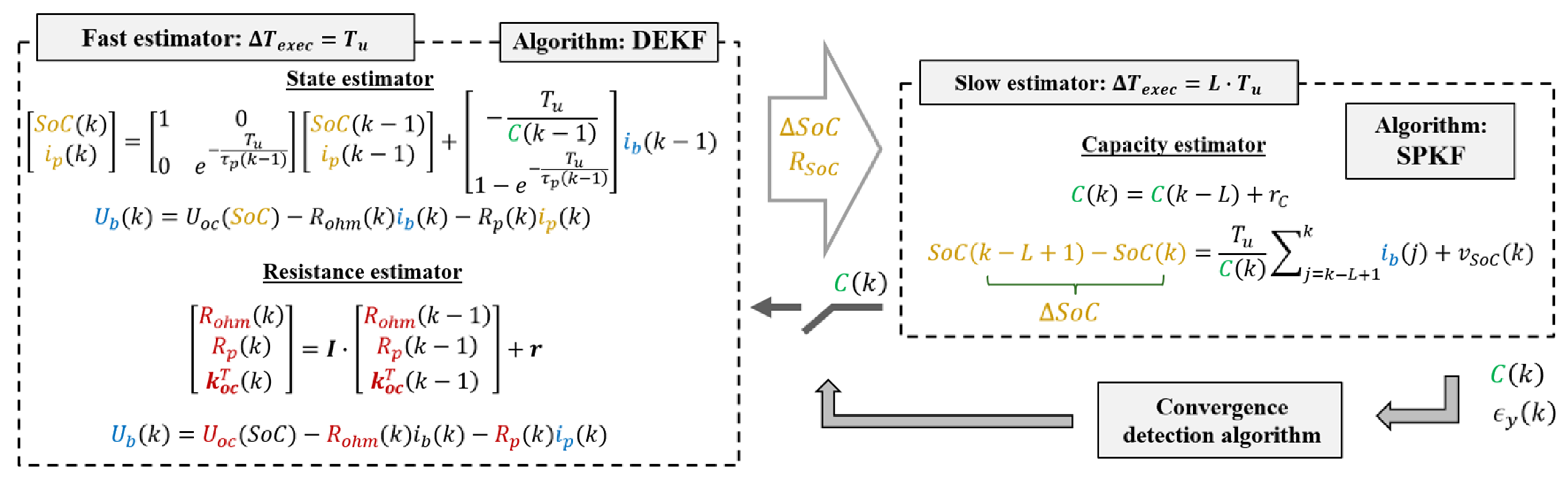
The model output is the SoC difference between two capacity estimates, while its input is the cumulative sum of battery current between those time instances. The SoC, as an output term, cannot be measured, but can be estimated by using the previously designed DEKF (both, estimates of SoC mean value and its variance are available). By looking at Equation (13) it can be seen that capacity estimate cannot be updated at the same rate as DEKF, because the signal-to-noise ratio of SoC estimate would be too low for the SoC dynamics being much slower than the current dynamics. The capacity estimator is therefore executed every
time steps, where
is in the range of 600–6000, i.e., 1 to 10 min. The overall estimator, i.e., the previously discussed DEKF extended with the capacity estimator, is shown in
Figure 8.
5.2. SPKF-Based Capacity Estimator
Since the battery capacity model output equation is distinctively nonlinear, the EKF-based estimator application has been found to give too noisy estimates with slow convergence rate. This is an expected result since EKF uses analytic linearization through Taylor series expansion around the current operating point, i.e., around the state variable (in this case capacity
) mean value. Another, more coherent approach to this problem is statistical linearization which linearizes the model at multiple points drawn from prior distribution of
. The estimator derived using this approach is called SPKF [
3]. There is a couple of SPKF versions which differ in calculation of sigma-points for linearization; in this paper, the method called central-difference Kalman filter (CDKF) is used because it provides simple parametrization without compromising accuracy [
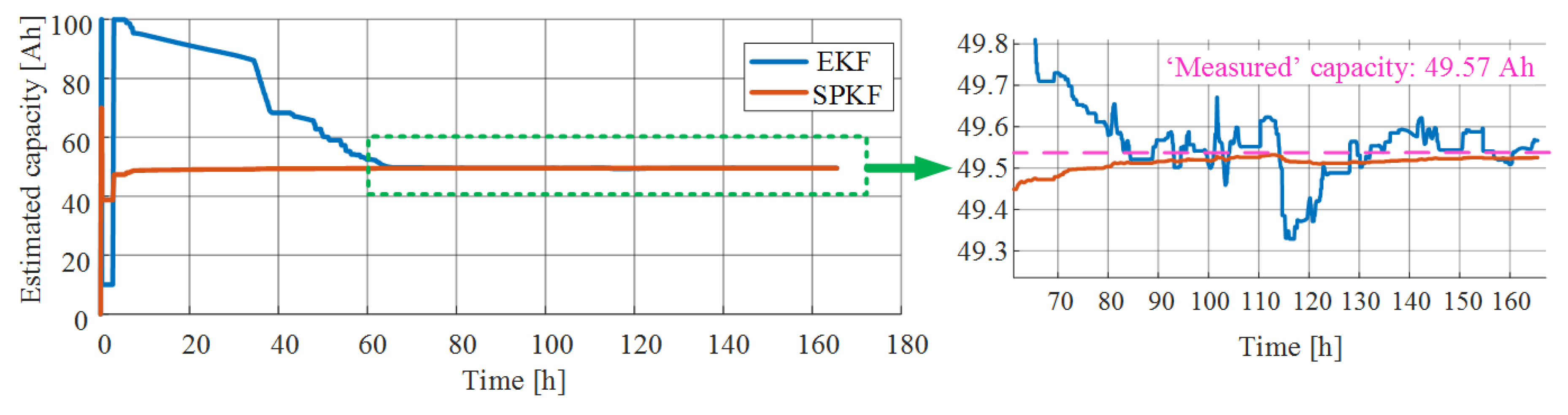
3]. Comparison between EKF- and SPKF-based capacity estimation, shown in
Figure 9, clearly illustrates the benefits of using SPKF when compared to EKF.
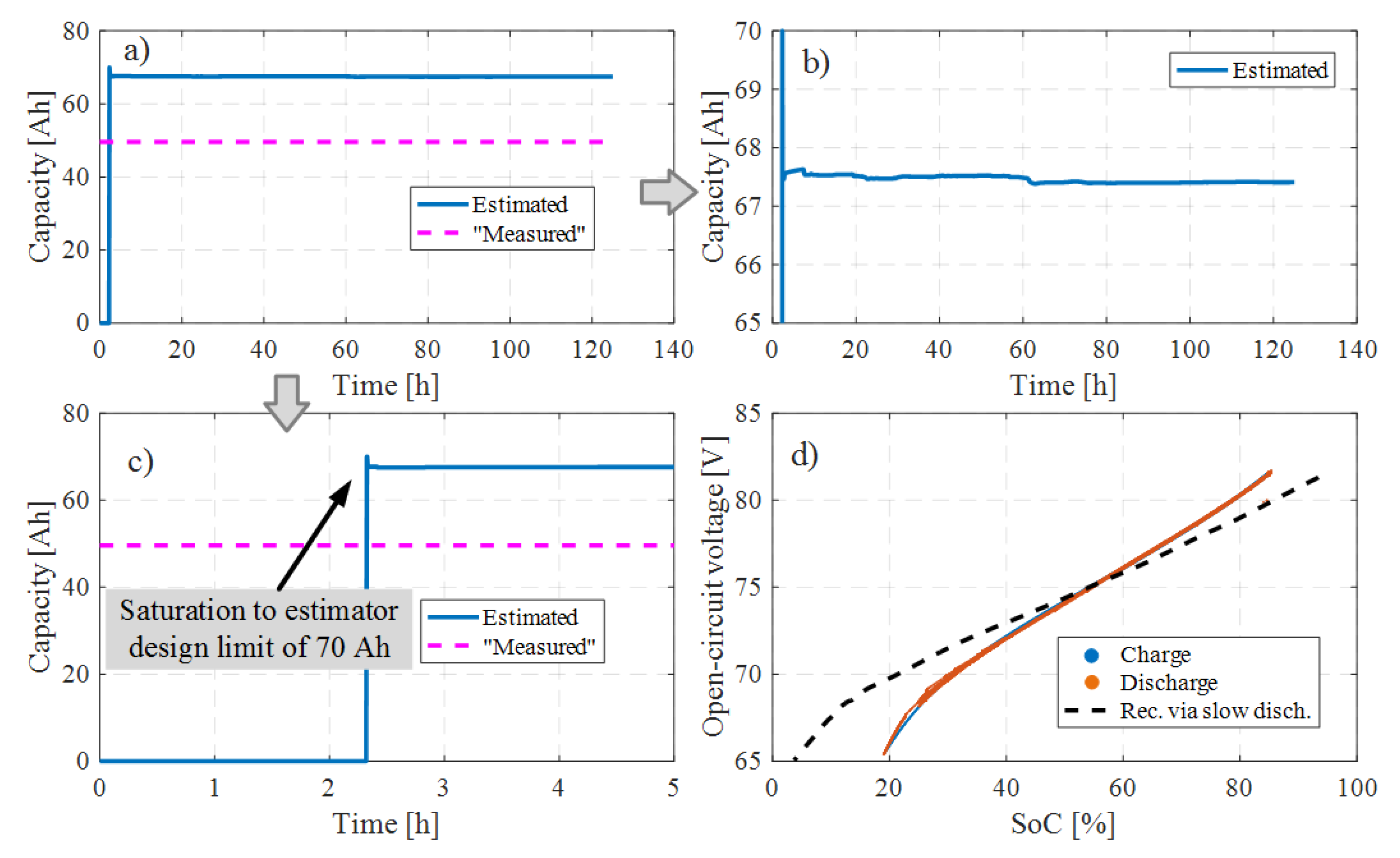
It is important to note that in the case shown in
Figure 9 the capacity estimates were not fed back into the state model of the DEKF, i.e., into Equation (6). If this were the case, i.e., if the state model of DEKF was updated with capacity estimates every
time stamps, the estimator would not converge to correct estimates, as shown in
Figure 10a–c. This is because every model parameter is estimated in a coupled manner, so there are multiple parameter combinations where output voltage residual would be minimized. For instance,
Figure 10d shows an estimate of
which is narrower than the actual curve, because the capacity is estimated higher than the actual one.
The capacity estimate feedback to the DEKF should be, therefore, turned on with some delay, i.e., until capacity estimate convergence is detected. For that purpose, capacity convergence detection algorithm has been designed, as presented in the next subsection.
5.3. Capacity Convergence Detection Algorithm
The capacity convergence detection algorithm is based on monitoring of the normalized estimation error (NEE) [
28]:
where
is the SoC estimate generated by the DEKF,
is the SoC calculated from the SPKF model output, and
is the SPKF innovation matrix (which is regularly calculated as a part of SPKF; note that it is a scalar in the particular case of single estimated parameter—the capacity). The convergence algorithm monitors the NEE, and when it is lower than some predefined value during some predefined number of consecutive time steps, the convergence is claimed.
5.4. Capacity Estimation Results
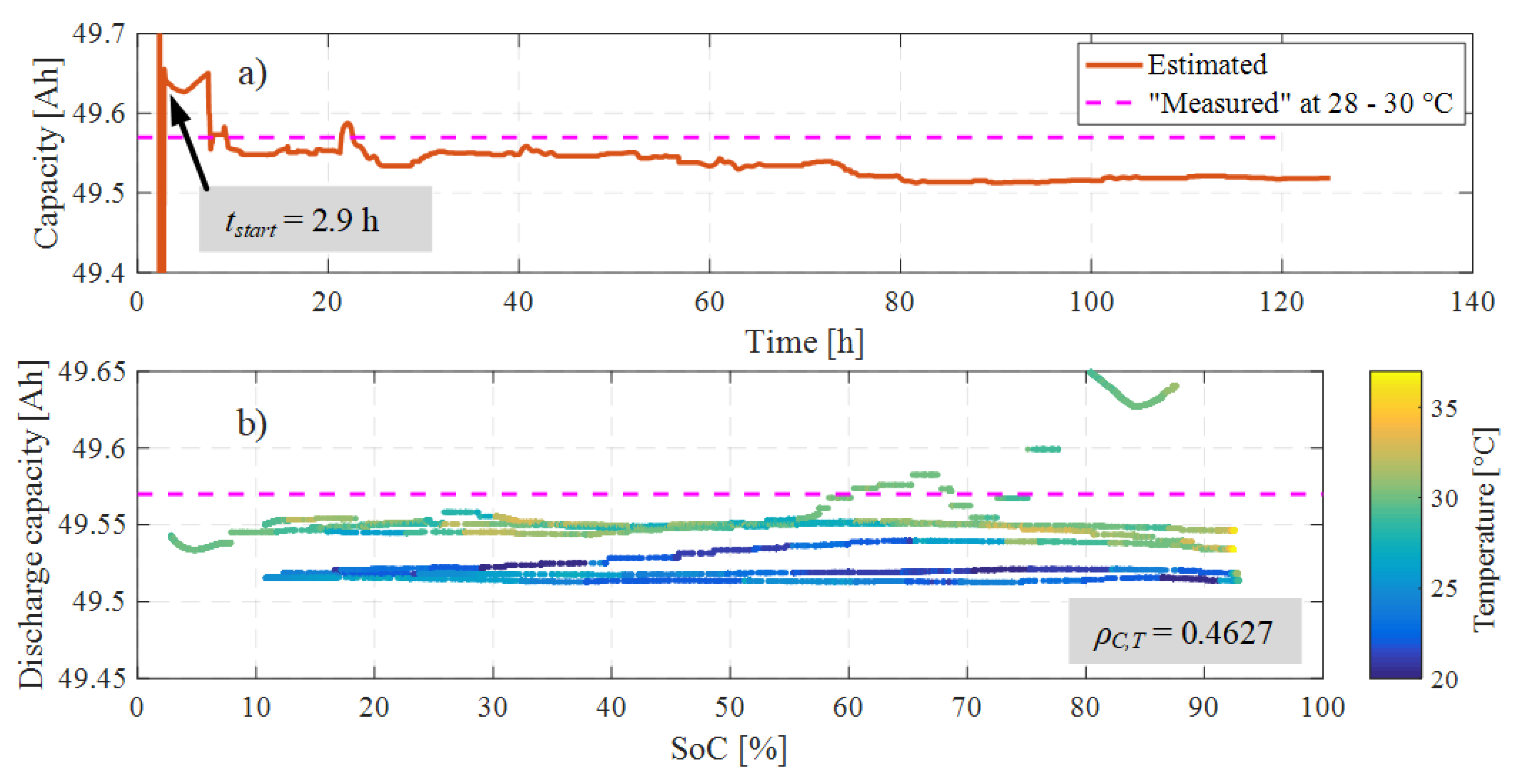
Results of SPKF-based capacity estimation algorithm with delayed and automatically calculated (through capacity convergence detection algorithm) start of capacity update (i.e.,
) within the DEKF state model (version with hysteresis model included was used) are shown in
Figure 11. The capacity estimates plotted versus time are shown in
Figure 11a along with the “measured” capacity (see
Figure 3b for details about capacity identification). Capacity convergence has automatically been detected after 2.9 h and from that point on, SPKF has been coupled to the DEKF.
Figure 11b shows capacity estimates during the discharge periods plotted versus SoC and color-mapped with respect to temperature. Capacity shows expected (based on the [
29]) positive correlation with the temperature.
Figure 12 shows the same plots as in the case of
Figure 6, but instead of using the adaptation mechanism the estimator relies on the explicit hysteresis model and has the capacity estimation included. The voltage residual is shown in
Figure 12a together with the usual statistics. This residual has higher
Lstat value than the one from
Figure 6a, which may be explained by the influence of added capacity estimation. The estimates of
and
, plotted in
Figure 12b,d with respect to SoC and temperature, respectively, are similar to those from
Figure 6b,d, but with slightly higher correlation with temperature for both resistances. Finally, it should be noted that there are no distinguishable sets of estimated
curves in
Figure 12c (unlike in
Figure 6c), because estimated
now describes the central curve while the hysteresis is accounted for in the model (see
Figure 7 and Equations (10) and (11)). Estimated
is slightly larger than the recorded one (see
Figure 3c for details about
identification) because the latter is discharge
curve while we estimate the average
since hysteresis is explicitly modelled in this case. The overall estimation algorithm is parametrized as given in
Appendix A.
6. Conclusions
An algorithm for dual estimation of battery state-of-charge (SoC) and remaining charge capacity has been proposed, which is aimed to be accurate over the whole battery lifetime and real-driving conditions including varying ambient temperatures. This was achieved by simultaneous estimation of relevant battery degradation-dependent parameters such as internal resistances and parameters of open-circuit voltage vs. SoC characteristic, .
To this end, the dual extended Kalman filter-based SoC estimation algorithm has been extended to estimate parameters of the characteristic along with the resistance parameters. This extension allows the DEKF to adapt for variations and capture its hysteresis without explicitly modelling it. The latter can be useful in cases when the exact hysteresis profile is not known in advance or when it needs to be updated at the given state-of-health level without a specific identification experiment.
Next, a battery capacity estimator has been designed as a separate estimator, as it is based on a different model than the one that has been used in the DEKF design. Moreover, capacity estimation is meant to be executed on a significantly slower time scale than the DEKF. It has been shown that the EKF-based capacity estimator gives rather inconsistent estimates with a slow convergence rate, which is explained by a distinctively nonlinear capacity model. Capacity estimator has, therefore, been designed by using a sigma-point Kalman filter (SPKF). Furthermore, it has been demonstrated that SoC and capacity estimators (i.e., DEKF and SPKF, respectively) cannot be started in a coupled manner, unless it is ensured that both estimators have converged. A capacity convergence detection algorithm has, therefore, been designed to automatically couple the two estimators.
Finally, the overall estimator has been successfully verified based on real driving cycle data acquired by using a fully electric scooter equipped with a telemetry measurement system. The DEKF output voltage estimation residual distribution was confirmed to be close to the voltage measurement noise, while resistance estimates showed expected correlations with temperature. The estimated capacity was shown to be close to the measured one and expectedly correlated with temperature, as well.
Future work will be directed towards further extensions and verifications of the proposed estimator to account for temperature- and aging-dependent variations of the polarization time constant and further analyze the sensitivity of estimator for broader operating conditions (e.g., wider temperature range), respectively. The emphasis will be on using the estimator to track battery degradation features in support of modelling the battery degradation process.
Author Contributions
Conceptualization, J.D., F.M., and M.H.; Methodology, F.M., M.H., and J.D.; Software, F.M.; Validation, F.M., J.D., and M.H.; Writing—Original Draft Preparation, F.M.; Writing—Review and Editing, J.D. and M.H.; Supervision: J.D. All authors have read and agreed to the published version of the manuscript.
Funding
It is gratefully acknowledged that this work has been supported through a small-scale grant program of the University of Zagreb, related to the project entitled “Experimental Characterization of Electric Scooter Battery Pack Aging”, as well as through project “Advanced Methods and Technologies in Data Science and Cooperative Systems” (DATACROSS) of the Centre of Research Excellence within the University of Zagreb.
Conflicts of Interest
The authors declare no conflict of interest.
Abbreviations
| BMS | Battery management system |
| DEKF | Dual extended Kalman filter |
| ECM | Equivalent circuit model |
| EKF | Extended Kalman filter |
| KF | Kalman filter |
| NEE | Normalized estimation error |
| OCV | Open-circuit voltage |
| PF | Particle filter |
| SoC | State-of-charge |
| SoH | State-of-health |
| SPKF | Sigma-point Kalman filter |
Appendix A. Estimator Parameters
The overall estimation algorithm is parametrized as given in
Table A1.
Table A1.
List of estimator parameters.
Table A1.
List of estimator parameters.
| Parameter Description and Its Mathematical Notation | Value |
|---|
| Variance of estimation, | |
| Variance of estimation, | |
| Variance of estimation, | |
| Initial SoC, | |
| Initial polarization current, | |
| Initial polarization resistance, | |
| Initial polarization resistance, | |
| Initial parameter, | |
| Initial parameter, | |
| Initial parameter, | |
| Initial parameter, | |
| Initial parameter, | |
| Scaling factor of submatrix bump in adaptation mechanism (see Section 4.2.2) | |
| NEE threshold value (see Section 5.3) | |
| Consecutive time steps NEE has to be lower than the above threshold (see Section 5.3) | |
| Ratio between SPKF and DEKF sampling time, (see Section 5.1) | |
References
- Plett, G.L. Battery Management Systems, Volume II: Eqivalent-Circuit Methods; Artech House: London, UK, 2016. [Google Scholar]
- Waag, W.; Fleischer, C.; Sauer, D.U. Critical review of the methods for monitoring of lithium-ion batteries in electric and hybrid vehicles. J. Power Sources 2014, 258, 321–339. [Google Scholar] [CrossRef]
- Van Der Merwe, R.; Wan, E. Sigma-Point Kalman Filters for Probabilistic Inference in Dynamic State-Space Models. Ph.D. Thesis, OGI School of Science and Engineering, Portland, OR, USA, 2004. [Google Scholar]
- Plett, G.L. Extended Kalman filtering for battery management systems of LiPB-based HEV battery packs—Part 2. Modeling and identification. J. Power Sources 2004, 134, 262–276. [Google Scholar] [CrossRef]
- Xiong, R.; Sun, F.; Gong, X.; He, H. Adaptive state of charge estimator for lithium-ion cells series battery pack in electric vehicles. J. Power Sources 2013, 242, 699–713. [Google Scholar] [CrossRef]
- Plett, G.L. Sigma-point Kalman filtering for battery management systems of LiPB-based HEV battery packs. Part 2: Simultaneous state and parameter estimation. J. Power Sources 2006, 161, 1369–1384. [Google Scholar] [CrossRef]
- Ye, M.; Guo, H.; Cao, B. A model-based adaptive state of charge estimator for a lithium-ion battery using an improved adaptive particle filter. Appl. Energy 2017, 190, 740–748. [Google Scholar] [CrossRef]
- Severson, K.A.; Attia, P.M.; Jin, N.; Perkins, N.; Jiang, B.; Yang, Z.; Chen, M.H.; Aykol, M.; Herring, P.K.; Fraggedakis, D.; et al. Data-driven prediction of battery cycle life before capacity degradation. Nat. Energy 2019, 4, 383–391. [Google Scholar] [CrossRef]
- Baccouche, I.; Jemmali, S.; Manai, B.; Omar, N.; Essoukri Ben Amara, N. Improved OCV model of a Li-ion NMC battery for online SOC estimation using the extended Kalman filter. Energies 2017, 10, 764. [Google Scholar] [CrossRef]
- Chen, X.; Lei, H.; Xiong, R.; Shen, W.; Yang, R. A novel approach to reconstruct open circuit voltage for state of charge estimation of lithium ion batteries in electric vehicles. Appl. Energy 2019, 255, 113758. [Google Scholar] [CrossRef]
- Xiong, R.; Sun, F.; Chen, Z.; He, H. A data-driven multi-scale extended Kalman filtering based parameter and state estimation approach of lithium-ion olymer battery in electric vehicles. Appl. Energy 2014, 113, 463–476. [Google Scholar] [CrossRef]
- Yang, R.; Xiong, R.; He, H.; Mu, H.; Wang, C. A novel method on estimating the degradation and state of charge of lithium-ion batteries used for electrical vehicles. Appl. Energy 2017, 207, 336–345. [Google Scholar] [CrossRef]
- Tang, X.; Wang, Y.; Zou, C.; Yao, K.; Xia, Y.; Gao, F. A novel framework for Lithium-ion battery modeling considering uncertainties of temperature and aging. Energy Convers. Manag. 2019, 180, 162–170. [Google Scholar] [CrossRef]
- Li, S.; Pischinger, S.; He, C.; Liang, L.; Stapelbroek, M. A comparative study of model-based capacity estimation algorithms in dual estimation frameworks for lithium-ion batteries under an accelerated aging test. Appl. Energy 2018, 212, 1522–1536. [Google Scholar] [CrossRef]
- Plett, G.L. Recursive approximate weighted total least squares estimation of battery cell total capacity. J. Power Sources 2011, 196, 2319–2331. [Google Scholar] [CrossRef]
- Wei, Z.; Zhao, J.; Ji, D.; Tseng, K.J. A multi-timescale estimator for battery state of charge and capacity dual estimation based on an online identified model. Appl. Energy 2017, 204, 1264–1274. [Google Scholar] [CrossRef]
- Kasiński, P. GOVECS GROUP Supporting Role of IT for Lithium Ion Batteries Transportation and SOH Monitoring. Available online: http://fplreflib.findlay.co.uk/images/pdf/scms/Przemek GOVECS Berlin Summit.pdf (accessed on 15 September 2019).
- LEM CAB 300 Current Transducer Manual. Available online: http://media.ev-tv.me/CAB300-CSP3.pdf (accessed on 30 August 2019).
- Fleischer, C.; Waag, W.; Heyn, H.M.; Sauer, D.U. On-line adaptive battery impedance parameter and state estimation considering physical principles in reduced order equivalent circuit battery models part 1. Requirements, critical review of methods and modeling. J. Power Sources 2014, 262, 457–482. [Google Scholar] [CrossRef]
- Rodríguez, A.; Plett, G.L. Controls-oriented models of lithium-ion cells having blend electrodes. Part 1: Equivalent circuits. J. Energy Storage 2017, 11, 219–236. [Google Scholar] [CrossRef]
- Waag, W.; Käbitz, S.; Sauer, D.U. Experimental investigation of the lithium-ion battery impedance characteristic at various conditions and aging states and its influence on the application. Appl. Energy 2013, 102, 885–897. [Google Scholar] [CrossRef]
- Tang, X.; Wang, Y.; Yao, K.; He, Z.; Gao, F. Model migration based battery power capability evaluation considering uncertainties of temperature and aging. J. Power Sources 2019, 440, 227141. [Google Scholar] [CrossRef]
- Abdel Monem, M.; Trad, K.; Omar, N.; Hegazy, O.; Mantels, B.; Mulder, G.; Van den Bossche, P.; Van Mierlo, J. Lithium-ion batteries: Evaluation study of different charging methodologies based on aging process. Appl. Energy 2015, 152, 143–155. [Google Scholar] [CrossRef]
- Gibbs, B.P. Advanced Kalman Filtering, Least-Squares and Modeling; John Wiley & Sons: Hoboken, NJ, USA, 2011; ISBN 9780470529706. [Google Scholar]
- Barai, A.; Widanage, W.D.; Marco, J.; Mcgordon, A.; Jennings, P. A study of the open circuit voltage characterization technique and hysteresis assessment of lithium-ion cells. J. Power Sources 2015, 295, 99–107. [Google Scholar] [CrossRef]
- Wei, Z.; Zhao, J.; Zou, C.; Lim, T.M.; Tseng, K.J. Comparative study of methods for integrated model identification and state of charge estimation of lithium-ion battery. J. Power Sources 2018, 402, 189–197. [Google Scholar] [CrossRef]
- Baronti, F.; Femia, N.; Saletti, R.; Visone, C.; Zamboni, W. Hysteresis modeling in Li-ion batteries. IEEE Trans. Magn. 2014, 50, 1–4. [Google Scholar] [CrossRef]
- Li, X.R.; Zhao, Z.; Jilkov, V.P. Measures of Performance for Evaluation of Estimators and Filters—Semantic Scholar; International Society for Optics and Photonics: Bellingham, WA, USA, 2001. [Google Scholar]
- Farmann, A.; Waag, W.; Marongiu, A.; Sauer, D.U. Critical review of on-board capacity estimation techniques for lithium-ion batteries in electric and hybrid electric vehicles. J. Power Sources 2015, 281, 114–130. [Google Scholar] [CrossRef]
© 2020 by the authors. Licensee MDPI, Basel, Switzerland. This article is an open access article distributed under the terms and conditions of the Creative Commons Attribution (CC BY) license (http://creativecommons.org/licenses/by/4.0/).


