Abstract
In cyber–physical power systems (CPPSs), the interaction mechanisms between physical systems and cyber systems are becoming more and more complicated. Their deep integration has brought new unstable factors to the system. Faults or attacks may cause a chain reaction, such as control failure, state deterioration, or even outage, which seriously threatens the safe and stable operation of power grids. In this paper, given the interaction mechanisms, we propose an interdependent model of CPPS, based on a characteristic association method. Utilizing this model, we can study the fault propagation mechanisms when faulty or under cyber-attack. Simulation results quantitatively reveal the propagation process of fault risks and the impacts on the CPPS due to the change of state quantity of the system model.
1. Introduction
As one of the most complicated man-made systems in the world [1], a power system is a nation’s critical infrastructure that underpins national security and economic stability. In the last decade, smart grids have been emerging as the next-generation electrical power infrastructures [2]. With the development of many advanced technologies [3], such as advanced modern sensor and measurement technology, communication and information technology, computer technology, and control technology, traditional power grids are undergoing a series of changes from single power grids to CPPSs, which are composed of traditional power grids and cyber networks [4]. Smart grids can allow for bidirectional information flow [5] and they depend significantly more on data transfers than traditional electric power grids. Smart cyber systems provide better monitoring, transferring, and controlling functions for physical systems [6], but there is nonetheless a trade-off, as risks then not only threaten the physical systems themselves but also the cyber systems. The addition of cyber infrastructures may lead to a grid that fails more frequently, with more severe consequences [7]. Furthermore, increased complexity and connectivity are likely to enlarge the scope affected by accidental faults or malicious attacks [7]. As a result, to guarantee the robustness of the whole system, it is of considerable significance to research the interaction mechanisms between the cyber systems and the physical systems.
Essentially, in CPPSs, physical systems refer to electric networks that perform power generation, transmission, and distribution tasks, while cyber systems refer to communications and computational nodes, which monitor, protect, and control the physical electrical systems. In other words, the cyber infrastructure touches almost every part of the modern power system [8]. However, despite employing modern technologies and bringing promising economic benefits, the existing CPPS does not exhibit the high dependability required by infrastructure tasked with fulfilling the critical needs of modern society [9]. Several power outages worldwide, such as the physical attack incident on the California electric power substation [10] in April 2013 by unidentified gunmen, and the cyber-attack incident that resulted in Venezuela’s power grid suffering a blackout in March 2019, have attracted much attention [11]. Therefore, with the increased cyber–physical vulnerabilities of contemporary power grids, it is extremely important to analyze the fault propagation mechanisms between cyber systems and physical systems for effectively defending the blackouts and increasing the safety and dependability of the whole cyber–physical power system.
Some recent studies have focused on analyzing the propagation features of cascading failures. The studies in [12,13,14,15] only consider the pure topological indices of the electric power transmission networks to assess the vulnerability of power systems. However, these approaches are far from power dynamics in power transmission systems, because they largely ignore the electric system properties, such as the power flow. Combining the pure topological indices and electric system properties, the cascading failures can be mimicked more accurately, which provides a new way to analyze the propagation features of cascading failures. Based on a simplified interaction graph representation of cascading outages, a PageRank-based algorithm is proposed to identify the vulnerable lines in power grids [16]. By calculating the probability that one component failure causes another, an interaction model considering power flow and re-dispatching is proposed to mitigate the cascading failure risk [17]. By adding the operational features of an electric network to form the temporal information of the network, a cascading faults graph is proposed to reveal the mechanism of fault propagation [18]. Taking active and reactive loads into consideration, a model is devised to balance the loads between edges connected with the same node for preventing the occurrence of cascading failures [19]. Nevertheless, the above approaches based on the complex network theory merely analyze the failures of power networks, and furthermore, ignore the influence of the cyber networks.
As a matter of fact, it is incomprehensible to consider analyzing physical faults or cyber faults separately. The separate analysis does not take into account the interactions between networks. In terms of the difference in the nodes and edges, an interdependent model between power systems and dispatching data networks is proposed to investigate only the cascading failures [3], rather than the fault transmission process between power grids and cyber networks. The above work is analyzed from the pure topological complex networks viewpoint employing the undirected and unweighted model without calculating electric system properties and propagation characteristics of the cyber network. Taking active power flow properties into consideration, a CPPS model is proposed to study the impacts of cyber component faults on the failures of a power network [20]. However, the impacts of cyber networks, such as Routing strategy, have not been considered. Multiple studies in [21,22] assess the risk propagation mechanism from the perspective of the communication specialty. These approaches identify cyber secure vulnerabilities in terms of terminal equipment and communication protocols. This type of research does not combine information transmission with the dispatch control of the power grid, which ignores the operating characteristics of the power grid and the interaction characteristics in CPPSs. Through integrating different simulation platforms, the hybrid agent-based modeling approach is proposed to model interdependencies between physical systems and cyber systems [23]. The hybrid agent-based modeling simulation scheme mainly has difficulties in time synchronization and heavy computational burdens.
In this paper, we propose a practical cyber–physical power system model to describe the interaction characteristics of the power sides and cyber sides, which takes into account the topological structure and electric characteristics. Then, to depict the cascading failure process and suppress the spread of the cascading failures, we introduce a fault propagation mechanism analysis method which considers the interactions between physical networks and cyber networks. The main contributions of this paper are summarized as follows:
- By investigating the interaction mechanism between the physical system and the cyber system, the interdependent model of CPPS is proposed in terms of the characteristic association method and interdependent network theory, which can reduce the computational complexity of modeling.
- Incorporating cyber system faults, physical system internal faults and their coupled system faults, the analysis of the fault propagation mechanism is introduced to simulate the failure regularity of components and the interactions between the components.
The remainder of this paper is organized as follows: a framework of the cyber–physical interdependent network is presented in Section 2. In Section 3, the interdependent model of the cyber–physical power system is proposed. The fault propagation mechanisms for the CPPS are analyzed in Section 4. Case studies and results analysis are presented in Section 5. Finally, Section 6 has the conclusions of the paper.
2. Framework of Cyber–Physical Interdependent Networks
The transmission lines and electrical elements can be converted into branches and nodes respectively. Power networks are therefore sets of branches and nodes. The communication lines and communication elements can be converted into edges and nodes respectively. Similarly, cyber networks are a set of edges and nodes. Some of the nodes in power networks can exchange and share data with some of the nodes in cyber networks. These nodes are called dependent nodes. The edges that can exchange data among the dependent nodes are called interdependent edges. The networks composed of interdependent nodes and interdependent edges are called coupled networks.
The network topology is the connection mode among the nodes. The topology of power systems and cyber systems can be represented by the connection mode between nodes and branches. In power networks, the node types contain generator nodes, load nodes, transformer nodes, branch breaker nodes, sensor nodes, and processor nodes. In cyber systems, the node types contain cyber nodes and control centers.
Based on the framework of the interdependent network, the architecture of the cyber–physical interdependent network is shown in Figure 1. In this architecture, sensors collect operating data of power grids and transmit it to cyber nodes. After gathering information from all cyber nodes, the control center will make decisions and send control command information to cyber nodes. Processors receive control instructions from cyber nodes and subsequently execute instructions. Furthermore, to describe the transmission direction of the information between networks, we define the uplinks, the direction of which is from the power network to the control center. The downlinks are opposite to the uplinks, the direction of which is from the control center to the power network.
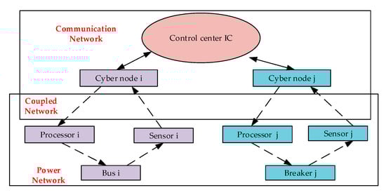
Figure 1.
Architecture of cyber–physical interdependent network.
3. Interdependent Model of Cyber–Physical Power System
According to Figure 1, the cyber–physical interdependent network can be divided into three sub-networks: power network, cyber network, and coupled network. In this section, each of the sub-networks is firstly modeled. By utilizing the incidence matrix to combine three sub-networks models, we propose an integrated model of the cyber–physical power system. The detailed modeling descriptions are presented below.
3.1. Modeling of Sub-Networks in Cyber–Physical Interdependent Networks
3.1.1. Modeling of the Power Networks
As previously mentioned, the power networks we modeled are based on the DC power flow. The cyber networks only have impacts on the power injections at buses and the power flows in branches. The power injections at power buses can be modeled as:
where P is a vector of the power injections at buses, B is the node susceptance matrix of a power grid, and θ is a vector of the phases at all buses.
The power flows in power branches are written as:
where F is an antisymmetric matrix of the power flows in branches, A denotes a square matrix in which all elements are 1, diag(θ) represents a diagonal matrix with the elements of θ on the main diagonal, and ‘◦’ represents Hadamard product.
Combining Equations (1) and (2), we have
where diag(P) represents a diagonal matrix with the elements of P on the main diagonal. The diagonal elements of Ppower denote the power injections at buses and other elements denote the power flows in branches.
Operation data of the physical system include topology information besides power information. The relations between two buses in the power network are expressed by:
where indicates bus i and bus j are connected, otherwise .
Moreover, according to the aforementioned architecture described in Figure 1, in a highly intelligent power system, each of the electric devices is equipped with sensors and processors. Sensors collect the power information from the physical system and processors send various operating commands to the physical system. The sensor nodes are represented as:
where each element of Cs equals 0 or 1. Specifically, if bus i is equipped with a sensor, csii = 1, or else csii = 0. If the branch (i,j) with i ≠ j is equipped with a sensor, csij = csji = 1, or else csij = csji = 0.
Likewise, the processor nodes are defined as:
where each element of Pc equals 0 or 1. Specifically, if bus i is equipped with a processor, pcii = 1, or else pcii = 0. If the branch (i,j) with i ≠ j is equipped with a processor, pcij = pcji = 1, or else pcij = pcji = 0.
3.1.2. Modeling of Coupled Networks
We suppose that the transmitted data are unchanged between sub-networks. According to the definition of uplinks and downlinks in the preceding section, as the physical system is fully coupled with the cyber system, the uplinks in the coupled network are where the physical information collected from sensors in the physical system are transmitted to cyber nodes in the cyber system. Simultaneously, the downlinks in the coupled network are where the operation commands sent from cyber nodes in the cyber system are transmitted to processors in the physical system.
To depict if there are uplinks between physical systems and cyber systems, a matrix Oup is:
where each element of Oup equals 0 or 1. More precisely, if there is an uplink between the sensor of bus i and a cyber node, Ouii = 1, or else Ouii = 0. If there is an uplink between the sensor of the branch (i,j) and a cyber node, Ouij = Ouji = 1, or else Ouij = Ouji = 0.
The downlinks in the coupled system can be expressed by:
where each element of Odown equals 0 or 1. More precisely, if there is a downlink between the processor of bus i and a cyber node, Odii = 1, or else Odii = 0. If there is a downlink between the processor of the branch (i,j) and a cyber node, Odij = Odji = 1, or else Odij = Odji = 0.
3.1.3. Modeling of Cyber Networks
Cyber network modeling includes cyber node modeling, the uplink of cyber system modeling, downlink of cyber system modeling and the control center modeling. According to the aforementioned framework, each of the cyber nodes is connected to each of the physical nodes one by one.
The operation states of cyber nodes are described by:
where each element of Cn equals 0 or 1. More precisely, if a cyber node connected to bus i is in the normal operation state, cnii = 1, or else cnii = 0. If a cyber node connected to the branch (i,j) is in the normal operation state, cnij = cnji = 1, or else cnij = cnji = 0.
Similar to the definition of uplinks and downlinks in the coupled network, we define the uplinks in the cyber system as the physical information collected from cyber nodes uploaded to the control center. Analogously, the downlinks in the cyber system are the operation commands sent from the control center downloaded to processors.
The uplinks between cyber nodes and the control center are given by:
where each element of Tup equals 0 or 1. More precisely, if there is an uplink between the control center and a cyber node connected to the sensor of bus i, then tuii = 1, or else tuii = 0. If there is an uplink between the control center and a cyber node connected to the sensor of the branch (i,j), then tuij = tuij = 1, or else tuij = tuij = 0.
The downlinks in the cyber system are depicted by:
where each element of Tdown equals 0 or 1. More precisely, if there is a downlink between the control center and a cyber node connected to the sensor of bus i, then tdii = 1, or else tdii = 0. If there is a downlink between the control center and a cyber node connected to the sensor of the branch (i,j), then tdij = tdji = 1, or else tdij = tdji = 0.
The control center is the core node of the cyber system and provides guarantees for the security and stability of the physical system. Based on the monitoring data of the physical system collected from sensors, the control center analyzes the operation state of the physical system, then calculates the power flow of the physical system, finally making the optimal control decision on the basis of the state of the whole cyber–physical power system, and sends control commands to processors.
The monitoring data received from the physical system mainly includes power flows and topology information of the physical system, which are defined as and respectively. The and can be calculated using
The commands sent from the control center mainly contain the control commands for buses and branches, which are defined as and . The is
where is the change of power for bus i. To be more specific, if , it is the command that the output should be increased for the generator connected to bus i, or else it is the command that the output should be decreased for the generator connected to bus i.
The can be handled conveniently by:
where is the adjustment of the breaker’s condition for the branch (i,j). We stipulate that if , then the breaker of the branch (i,j) is closed. If , the breaker of the branch (i,j) is open.
3.2. Integrated Model of Cyber–Physical Interdependent Networks
The equations of each sub-network are used only for calculating the operation state of the internal network individually, which cannot reflect the real-time interaction between power networks and cyber networks. By incorporating the characteristics of three sub-networks, the integrated model of the interdependent network is computed by:
where
and H is the generalized decision function of the control center, is the revised power injection matrix of power network, is the revised incidence matrix of the power network, is a revised vector of the power injections at power buses, is a revised admittance matrix, is a revised vector of the phases at all buses and is a revised power injections in power branches.
4. Fault Propagation Mechanism Analysis in CPPS
For the CPPS system, any faults or attacks may cause control failure or even widespread blackouts, which bring negative effects on the reliability and safety of system operations. It is essential to analyze the propagation paths of cascading faults for providing safe operation.
The fault propagation of the power system can be evaluated by the N − 1 method, which scans all possible electrical property failures and analyzes the cyber–physical system responses corresponding to each physical fault. Likewise, this idea can be implemented equally to cyber fault propagation analysis. In cyber systems, cyber faults are mainly caused by cyber-attacks, which lead the system to generate improper control commands that affect the physical system. Utilizing the interdependent model of CPPS detailed in the last section, we analyze the faults from three sub-networks respectively and investigate the CPPS system states under each fault in this section.
4.1. Fault Propagation Mechanisms from the Cyber System Faults
The characteristics of the cyber system are determined by the cyber transmission channel modeling and system topology. More recent studies have shown that the weak links of the cyber system mainly including cyber nodes and cyber channels are quite vulnerable to cyber-attacks. Thus, in terms of the targets of cyber-attacks, the fault propagation can be divided into two categories, which are cyber-attacks on the cyber nodes as well as cyber-attacks on the cyber transmission channels. As a result, we need to analyze these two types of fault propagation respectively.
4.1.1. Cyber-Attacks on Cyber Nodes
The cyber-attacks on cyber nodes in CPPSs refer to the damage to the local system due to the access rights of the cyber system obtained by an attacker, or the intentional destruction of equipment because of manual misoperation.
Cyber node failures are equivalent to unlinking cyber nodes, which will result in the control center not being able to obtain the operating status of the power grid in a timely manner and sense the potential operational risks. The detailed descriptions for cyber-attacks on the cyber nodes are presented below.
The cyber node attack matrix is built as:
where all the elements in equal 0 or 1. More specifically, is 0 if there exists a cyber-attack on the cyber node connected to bus i. is 1 if the cyber node connected to bus i is in the normal operation state. and are 0 if there exists a cyber-attack on the cyber node connected to the branch (i,j). and are 1 if the cyber node connected to the branch (i,j) is in the normal operation state.
After cyber-attacks on cyber nodes, the integrated calculating modeling in the interdependent network will be:
4.1.2. Cyber-Attacks on Cyber Channels
The cyber-attacks on communication transmission channels refer to when an attacker attacks the cyber network channels continuously and actively to disrupt communication availability and compromise the integrity of data, which leads to transmission channel blocking or channel data tampering. Depending on the different means of attacks, the cyber channel attacks mainly include denial of service attacks (Dos attacks) and false data injection attacks (FDI attacks). Then we need to quantitatively analyze the impacts of these two types of cyber channel attacks on the cyber system respectively.
1. Denial of service attack
The Dos attack is a resource exhaustion attack that sends numerous useless requests to exhaust the resources of the attacked object, such as network bandwidth, making the control center unable to communicate with the cyber nodes and information cannot be received or delivered normally, which can even result in data loss. Consequently, the analysis of the operation state and dispatching control of the control center is affected, thereby threatening the safe operation of the CPPS. In order to explain the influences of Dos attacks in more detail, we will separately analyze the Dos attacks on uplink and downlink below.
The uplink Dos attack matrix is modeled as:
where all the elements in equal 0 or 1. More specifically, is 0 if there is a Dos attack on an uplink between the control center and a cyber node connected to bus i. Otherwise, if this uplink is in the normal operation state, is 1. and are 0 if there exists a Dos attack on an uplink between the control center and the cyber node connected to the branch (i,j). Otherwise, if this uplink is in the normal operation state, and are 1.
The downlink Dos attack matrix is denoted by:
where all the elements in equal 0 or 1. More specifically, is 0 if there is a Dos attack on a downlink between the control center and a cyber node connected to bus i. Otherwise, if this downlink is in the normal operation state, is 1. and are 0 if there exists a Dos attack on a downlink between the control center and the cyber node connected to the branch (i,j). Otherwise, if this downlink is in the normal operation state, then and are 1.
After the Dos attacks, the integrated calculating modeling in the interdependent network will be changed and can be derived from:
2. False data injection attack
The FDI attack is an attack that injects erroneous data, such as incorrect monitoring data, on the uplinks or illegal tampering with data, such as grid control commands, on the downlinks, which hinders the reliability and accuracy of normal data exchange in the physical system. The ultimate goal of the FDI attack is to make the control center misunderstand the physical system state and then employ the wrong strategy, which affects the normal dispatching control of the physical system. We will separately analyze the FDI attacks on uplinks and downlinks below.
(1) FDI attacks on uplinks: As previously mentioned, the monitoring data that the control center will receive include two different types of information, namely power flow and topology information of the physical system. The uplink power injection attack matrix is represented by:
where the main diagonal element is 0 if there is not a power injection attack on an uplink between the control center and a cyber node connected to bus i. The elements and are 0 if there is not a power injection attack on an uplink between the control center and the cyber node connected to the branch (i,j). On the contrary, if there is a power injection attack on an uplink between the control center and a cyber node connected to bus i, the element is:
where λ1 is the false uplink power information that the control center will receive, which represents the attackers’ desired uplink power injection attack effect. Analogously, if there is a power injection attack on an uplink between the control center and the cyber node connected to the branch (i,j), the elements and are:
The uplink topology injection attack matrix is signified by:
where all the main diagonal elements in are 0. The elements and are 0 if there is not a topology injection attack on an uplink between the control center and the cyber node connected to the branch (i,j). Otherwise, if there is a topology injection attack on this uplink, the elements and are:
where λ2 is the false uplink topology information that the control center will receive, which represents an attacker’s desired uplink topology injection attack effect. λ2 = 0 means that the breaker is altered to open by the attacker and λ2 = 1 means that the breaker is altered to close by the attacker.
(2) FDI attacks on downlink: As previously mentioned, the control commands sent from the control center mainly contain the change of power for buses and adjustments of the breaker’s condition for branches.
The downlink power injection attack matrix is expressed by:
where is a diagonal matrix. The element in is 0 if there is not a power injection attack on a downlink between the control center and a cyber node connected to bus i. On the contrary, if there is a power injection attack on a downlink between the control center and a cyber node connected to bus i, then the element is:
where η1 is the false downlink power, which is the change of power for bus i altered by the attacker.
The downlink topology injection attack matrix is written as:
where the main diagonal elements in are 0. The elements and are 0 if there is not a topology injection attack on a downlink between the control center and the cyber node connected to the branch (i,j). Otherwise, if there is a topology injection attack on this downlink, the elements and are
where η2 is the false downlink topology information that represents the attackers’ desired downlink topology injection attack effect. η2 = 0 means that the breaker is altered to open by the attacker and η2 = 1 means that the breaker is altered to close by the attacker.
After the FDI attacks, the integrated calculating modeling in the interdependent network can be formulated as:
4.2. Fault Propagation Mechanisms from Physical System Internal Faults
4.2.1. Power Branch Fault
Since the operation modes of the power system are constantly changing, the node susceptance matrix of the power network will also change accordingly. If the node susceptance matrix is reconstructed for the changed network, the amount of calculation will be increasing dramatically. However, the change of power in a branch only has impacts on the self-admittance of the buses on both sides of the branch and the mutual admittance between two buses. As a result, it is unnecessary to rebuild the node susceptance matrix corresponding to the new operating condition. A new matrix can be obtained by simply modifying the original susceptance matrix.
As for Equation (1), when a fault occurs in the branch (i,j) between bus i and bus j, causing a break in that branch, it is equivalent to adding a branch with susceptance of bij between bus i and bus j. In this case, the number of buses and dimension of node susceptance matrix is unchanged. On the contrary, some elements in the susceptance matrix need to be modified. The self-susceptance increments of bus i and bus j are described by:
where and are the self-susceptance increments of bus i and bus j respectively.
The mutual susceptance increments between bus i and bus j are signified by:
where and are the mutual susceptance increments between bus i and bus j.
According to Equations (49) and (50), the self-susceptances of bus i and bus j will be changed:
where and are the original self-susceptances of bus i and bus j respectively, while and are the modified self-susceptances of bus i and bus j after branch fault respectively.
The modified mutual susceptances between bus i and bus j are:
where is the original mutual susceptance between bus i and bus j, and and are the modified mutual susceptances between bus i and bus j after the branch fault, respectively.
Hence, the node susceptance admittance matrix is modified as:
where is the susceptance matrix after branch faults, is the original susceptance matrix, is the increment matrix of susceptance.
After the branch faults, the power network modeling will be determined by:
4.2.2. Bus Fault
Once a bus fault occurs, the branches connected to this bus will be broken, which causes the disconnection with the whole power network. As a result, the topology structure of the power network is altered. In this case, the node susceptance matrix of this power network needs to be reconstructed for the changed topology.
We set the power network has N bus, and bus i in this network is connected to bus j as well as bus k. If bus i has a fault, its corresponding elements in the node susceptance matrix need to be modified. Specifically, if the dimension of the admittance matrix decreases to N − 1, then the elements of the ith column and ith row in the susceptance matrix need to be removed. This is except for bus i, as those buses connected to bus i need to be modified. According to the assumption before, the self-susceptance increments of bus j and bus k are represented as:
where is the original mutual susceptance between bus i and bus j, is the original mutual susceptance between bus i and bus k, is the self-susceptance increment of bus k.
According to Equations (58) and (59), the modified self-susceptances of bus j and bus k are calculated as:
where is the original self-susceptance of bus k, and are the modified self-susceptances of bus j and bus k after bus fault respectively.
Therefore, the node susceptance matrix is modified as:
where is the admittance matrix after bus faults.
After the bus faults, the power network modeling will be obtained by:
4.3. Fault Propagation Mechanisms from the Coupled System Faults
In the coupled network, coupled branches have a significant influence on the function of the whole interdependent network. The existence of coupled branches causes a single network to have different characteristics. The coupled system faults are mainly coupled branch faults. The coupled branch faults are equivalent to that of the coupled branches that are disconnected. As discussed in the previous section, coupled branches contain two types of branches, namely uplink coupled branches and downlink coupled branches. The uplink coupled branches are the topology connection between sensors and cyber nodes. The downlink coupled branches are the topology connection between cyber nodes and processors. In order to explain the impact of the coupled branch faults in more detail, we will separately analyze the coupled branch faults on uplinks and downlinks below.
The uplink coupled branch fault matrix is listed as:
where all the elements in equal 0 or 1. More specifically, is 0 if there is a fault on an uplink between a cyber node and a sensor connected to bus i. Otherwise, if this uplink is in the normal operation state, is 1. and are 0 if there exists a fault on an uplink between a cyber node and a sensor connected to the branch (i,j). Otherwise, if this uplink is in the normal operation state, and are 1.
The downlink Dos attack matrix can be equivalently represented by
where all the elements in equal 0 or 1. More specifically, is 0 if there is a fault on a downlink between a cyber node and a processor connected to bus i. Otherwise, if this downlink is in the normal operation state, is 1. and are 0 if there exists a fault on a downlink between a cyber node and a processor connected to the branch (i,j). Otherwise, if this uplink is in the normal operation state, and are 1.
After the coupled branch faults, the integrated calculating modeling in the interdependent network should be determined by:
5. Case Study
In this section, we will construct an interdependent model and propose some scenarios to demonstrate the effectiveness and superiority of fault propagation mechanism.
We take the IEEE-9 node system as an example, the structure and coupled cyber network of which is illustrated in Figure 2. Since the nine-bus power system is small and structurally symmetrical, this power network can be regarded as a unique region. In order to facilitate the analysis, it is essential to number the nodes. Bus numbers in the power network are from Bus 1 to Bus 9 and breaker numbers are from D1 to D9, which are the blue numbers in Figure 2. The corresponding cyber node numbers of buses and breakers are from I1 to I20, which are the yellow numbers in Figure 2. Moreover, the I in the cyber network represents the control center node, which is the brown number in Figure 2.
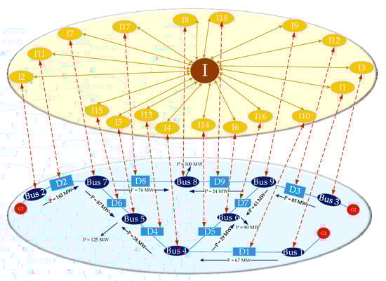
Figure 2.
Three-generator nine-bus power system and its cyber system.
Since the IEEE 9-node system fails to provide the power transfer limit of the line, we set the initial load rates of all the lines in the power system at 45% for the sake of analysis. Furthermore, Bus 1 is set as the balance bus.
According to the modeling methods in Section 3, , , , , , and can be modeled as:
In terms of the electric parameters of the IEEE-9 node system, when the CPPS operates normally, the original power flow distribution is:
5.1. Case 1
For the better description of the current system state and the system state which may be triggered at the next moment, the finite-state machine is introduced to simplify the logical description. We firstly analyze the fault propagation paths under the power branch fault and design the system state machine as shown in Figure 3.
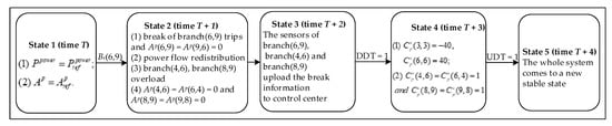
Figure 3.
State machine of branch fault state of cyber–physical power systems (CPPS).
As shown in Figure 3, and represent power flow and topology information when the physical system operates in a steady state. Br(6,9) represents a fault that occurred in the branch (6,9). The DDT is defined as uplinks of the cyber–physical coupled network in steady operation. If the uplinks of the cyber–physical coupled network operate in steady state, then DDT = 1, or else DDT = 0. The UDT is defined as downlinks of the cyber–physical coupled network in steady operation. If the downlinks of the cyber–physical coupled network operate in a steady state, then UDT = 1, or else UDT = 0.
First turning into state 1 in Figure 3, the system operates normally as illustrated in Figure 2 at time T. Assuming that a fault occurs on the branch (6,9), state 1 enters into state 2. In state 2, the breaker of the branch (6,9) trips at time T + 1 by reason of the branch fault, which leads to the power flow on each branch being redistributed. After the power flow redistribution, the breakers of branch (4,6) and branch (8,9) trip because of overload. After execution, state 2 enters into state 3 unconditionally. At time T + 2, the sensors of branch (6,9), branch (4,6) and branch (8,9) upload breaker information. If DDT = 1, then state 3 enters into state 4. In state 4, the control center will make decisions and send control commands after receiving the correct physical system information at time T + 3. The control commands include cutting off 40 MW in generation 3, load shedding 40 MW, and reclosing breaks of branch (4,6) as well as branch (8,9), which are , , and . If DDT = 1 and UDT = 1, then state 4 enters into state 5. In state 5, the physical system will come to a new stable state, as shown in Figure 4, after receiving the correct control commands at time T + 4. The power flow transferring from state 1 to state 5 in Figure 3 are given in Table 1.
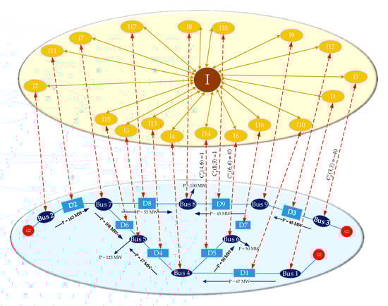
Figure 4.
The new stable state of CPPS after the branch fault.

Table 1.
The power flow transferring under power branch fault (MW).
5.2. Case 2
In case 2, we analyze the fault propagation paths under the power node fault and design the system state machine as shown in Figure 5.
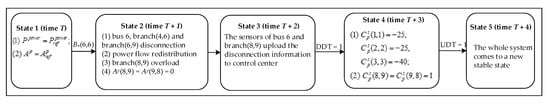
Figure 5.
State machine of node fault state of CPPS.
First turning into state 1 in Figure 5, the system operates normally, as shown in Figure 2, at time T. Assuming that a fault occurs on bus 6, which is represented by Bu(6,6), state 1 enters into state 2. In state 2, bus 6, branch (4,6) and branch (6,9) disconnect at time T + 1 on account of the bus fault, which leads to the power flow on each branch being redistributed. After the power flow redistribution, the breaker of the branch (8,9) trips due to overload. After execution, state 2 enters into state 3 unconditionally. At time T + 2, the sensors of bus 6 and branch (8,9) upload disconnection information. If DDT = 1, then state 3 enters into state 4. In state 4, the control center will make decisions and send control commands after receiving the correct physical system information at time T + 3. Those commands include cutting off 25 MW in generation 1 and generation 2, cutting off 40 MW in generation 3, and reclosing the break of branch (8,9), which is , , and . If DDT = 1 and UDT = 1, then state 4 enters into state 5. In state 5, the physical system will come to a new stable state, as shown in Figure 6, after receiving the correct control commands at time T + 4. The power flow transferring from state 1 to state 5 in Figure 5 is given in Table 2.
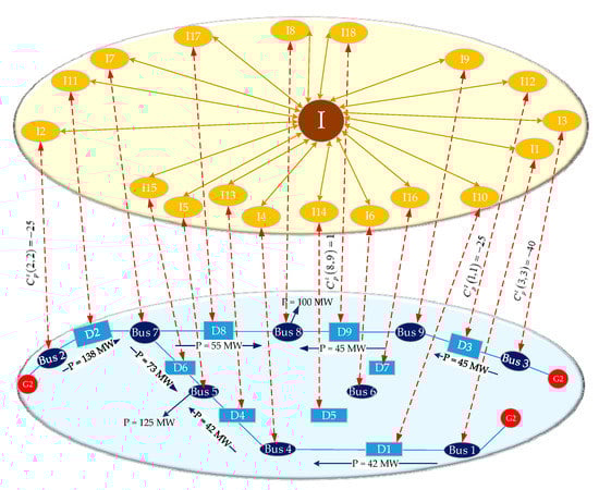
Figure 6.
The new stable state of CPPS after the bus fault.
Table 2.
The power flow transferring under bus fault (MW).
5.3. Case 3
In case 3, we analyze the fault propagation paths under the cyber system faults and design the system state machine as shown in Figure 7.
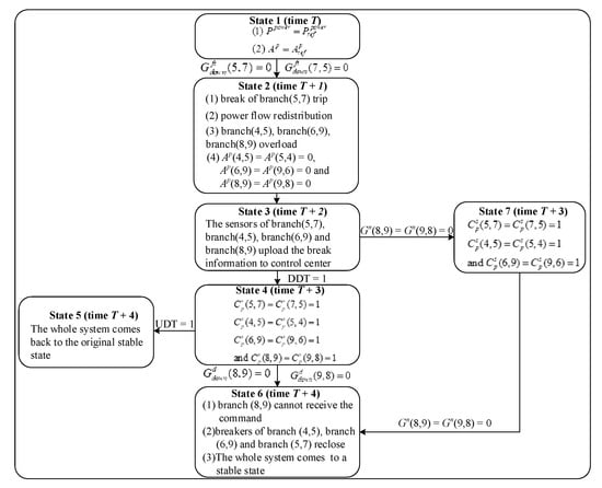
Figure 7.
State machine of cyber faults state of CPPS.
First turning into state 1 in Figure 7, the system operates normally, as shown in Figure 2, at time T. Assuming that an FDI attack occurs on the downlink between the control center and the cyber node connected to branch (5,7), which is represented by , state 1 enters into state 2. In state 2, the breaker of the branch (5,7) trips at time T + 1 by reason of the FDI attack, which leads to the power flow on each branch being redistributed. After the power flow redistribution, the breakers of branch (4,5), branch (6,9) and branch (8,9) trip because of overload. After execution, state 2 enters into state 3 unconditionally. At time T + 2, the sensors of branch (5,7), branch (4,5), branch (6,9) and branch (8,9) upload breakers information. If DDT = 1, then state 3 enters into state 4. In state 4, the control center will make decisions and send control commands after receiving the correct physical system information at time T + 3. Those commands include reclosing the breaks of branch (5,7), branch (4,5), branch (6,9) and branch (8,9), which are , , and . If DDT = 1 and UDT = 1, then state 4 enters into state 5. In state 5, the physical system will come back to the original stable state, as shown in Figure 2, after receiving the correct control commands at time T + 4. If a Dos attack occurs on the downlink between the control center and the cyber node connected to branch (8,9), which is represented by , then state 4 enters into state 6. In state 6, branch (8,9) cannot receive the command at time T + 4, which means that the breaker in branch (8,9) cannot reclose. The breakers of branch (4,5), branch (6,9) and branch (8,9) reclose and so that the whole system comes to a stable state. If there is a cyber-attack on the cyber node connected to branch (8,9), which is represented by , then state 3 enters into state 7. In state 7, the control center will make decisions and send control commands after receiving physical system information, except for the breaker information of branch (8,9) at time T + 3. Those commands include reclosing the breaks of branch (5,7), branch (4,5), and branch (6,9), which are , , and . Due to the cyber-attack on the cyber node connected to branch (8,9), state 7 enters into state 6. The power flow transferring from state 1 to state 6 in Figure 7 is given in Table 3.
Table 3.
The power flow transferring under cyber fault (MW).
5.4. Case 4
In case 4, we analyze the fault propagation paths under the coupled system faults and design the system state machine as shown in Figure 8.
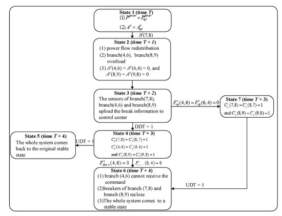
Figure 8.
State machine of coupled faults state of CPPS.
First turning into state 1 in Figure 8, the system operates normally, as illustrated in Figure 2 at time T. Assuming that the breaker of branch (7,8) suddenly trips, which is represented by Bt(7,8), state 1 enters into state 2. In state 2, due to the breaker trip, the power flow on each branch will redistribute at time T + 1. After the power flow redistribution, the breakers of the branch (4,6) and branch (8,9) trip because of overload. After execution, state 2 enters into state 3 unconditionally. At the time T + 2, the sensors of branch (7,8), branch (4,6) and branch (8,9) upload the breakers information. If DDT = 1, then state 3 enters into state 4. In state 4, the control center will make decisions and send control commands after receiving the correct physical system information at time T + 3. Those commands include reclosing breaks of branch (5,7), branch (4,5), branch (6,9) and branch (8,9), which are , and . If DDT = 1 and UDT = 1, then state 4 enters into state 5. In state 5, the physical system will come back to the original stable state in Figure 2 after receiving the correct control commands at time T + 4. If there is a coupled fault on a downlink between a cyber node and a processor connected to the branch (4,6), which is represented by , then state 4 enters into state 6. In state 6, the branch (4,6) cannot receive the command at time T + 4, which means that the breaker of branch (4,6) cannot reclose. The breakers of branch (7,8) and branch (8,9) reclose so that the whole system comes to a stable state. If there is a coupled fault on a downlink between a cyber node and a sensor connected to the branch (4,6), which is represented by , then state 3 enters into state 7. In state 7, the control center will make decisions and send control commands after receiving the physical system information, except for the breaker information of branch (8,9) at time T + 3. Those commands include reclosing the breaks of branch (5,7), branch (4,5), and branch (6,9), which are and . State 7 then enters into state 6. The power flow transferring from state 1 to state 6 is given in Table 4.
Table 4.
The power flow transferring under coupled faults (MW).
6. Discussion and Conclusions
This paper focuses on fault propagation in cyber–physical power systems, and presents an interdependent model and fault propagation mechanism analysis for the CPPSs. In terms of the interdependent theory, a framework of cyber–physical interdependent network that takes into account the communication transmission process is first proposed. Based on the system steady state and power flow equations, the modeling process is divided into three parts, which are the power networks, the cyber networks, and the coupled networks. Through effectively associating the power networks with the cyber networks, the integrated model of cyber–physical interdependent networks based on the multi-characteristics association method is proposed to explain the association relationship between power networks and cyber networks.
By analyzing the different locations of faults or attacks and defining the faults and attack matrixes, the parameterized characterization method of fault propagation in CPPS is proposed. To illustrate the theoretical approach presented in the paper, we take a CPPS model consisting of IEEE 9-bus system as an example to quantitatively deduce and analyze the risk propagation process of the faults or attacks in CPPSs.
The modeling and fault propagation analysis of CPPSs proposed in this paper has the following characteristics:
In the proposed model, the power network is modeled based on the DC model and the control center of cyber network generates decisions as well as controls the power and topology, which forms a closed loop. The CPPS modeling comprehensively considers the topology and electric characteristics, which meets the properties of power networks more adequately when compared with the model based on the complex network. The CPPS modeling takes into consideration the direction of information flow, which is more suitable for the power dispatching automation system. On the basis of the system steady state and power flow calculation, the proposed analysis method has low computational complexity when the topology of CPPSs is varied. Moreover, the formulations of the effects of typical faults under the integrated model framework can be implemented, which provides a new solution for the quantitative analysis of the impact of different types of faults on the CPPSs.
However, the modeling is based on DC instead of AC power flow. In addition, due to the simplicity of the test system, the power system comes to a steady state by power flow calculating no more than twice, which means that the risk communication process ends early. In the future, we will study the modeling approach in a larger scale system by AC power flows and compare their differences.
As for implementation potentials, we need to consider more communication factors and faults, such as the impact of different communication delays on the CPPSs. The real-time co-simulation scheme based on power system simulation software and communication system simulation software will be studied.
Author Contributions
Methodology, X.G.; formal analysis, X.G.; Resources, Y.T. and F.W.; visualization, X.G.; writing—original draft preparation, X.G.; writing—review and editing, X.X.; visualization, X.X.; manuscript revising, X.G., Y.T. and F.W.; funding acquisition, Y.T. All authors have read and agreed to the published version of the manuscript.
Funding
This research was funded by the National Natural Science Foundation of China under Grant No. 51577046, the State Key Program of National Natural Science Foundation of China under Grant No. 51637004, the national key research and development plan “important scientific instruments and equipment development” Grant No.2016YFF0102200, Equipment research project in advance Grant No.41402040301.
Conflicts of Interest
The authors declare no conflict of interest.
References
- Xiang, Y.; Wang, L.; Liu, N. A robustness-oriented power grid operation strategy considering attacks. IEEE Trans. Smart Grid 2018, 9, 4248–4426. [Google Scholar] [CrossRef]
- Yan, J.; He, H.; Zhong, X. Q-learning-based vulnerability analysis of smart grid against sequential topology attacks. IEEE Trans. Inf. Forensics Secur. 2016, 12, 200–210. [Google Scholar] [CrossRef]
- Cai, Y.; Cao, Y.; Li, Y. Cascading failure analysis considering interaction between power grids and communication networks. IEEE Trans. Smart Grid 2015, 7, 530–538. [Google Scholar] [CrossRef]
- Chen, Y.; Li, Y.; Li, W. Cascading failure analysis of cyber physical power system with multiple interdependency and control threshold. IEEE Access 2018, 6, 39353–39362. [Google Scholar] [CrossRef]
- Farraj, A.; Hammad, E.; Kundur, D. A cyber-physical control framework for transient stability in smart grids. IEEE Trans. Smart Grid 2016, 9, 1205–1215. [Google Scholar] [CrossRef]
- Cai, Y.; Chen, Y.; Li, Y. Reliability Analysis of Cyber–Physical Systems: Case of the Substation Based on the IEC 61850 Standard in China. Energies 2018, 11, 2589. [Google Scholar] [CrossRef]
- Marashi, K.; Sarvestani, S.S.; Hurson, A.R. Consideration of cyber-physical interdependencies in reliability modeling of smart grids. IEEE Trans. Sustain. Comput. 2017, 3, 73–83. [Google Scholar] [CrossRef]
- Davis, K.R.; Davis, C.M.; Zonouz, S.A. A cyber-physical modeling and assessment framework for power grid infrastructures. IEEE Trans. Smart Grid 2015, 6, 2464–2475. [Google Scholar] [CrossRef]
- Hines, P.; Apt, J.; Talukdar, S. Large blackouts in North America: Historical trends and policy implications. Energy Policy 2009, 37, 5249–5259. [Google Scholar] [CrossRef]
- Wei, L.; Sarwat, A.I.; Saad, W. Stochastic games for power grid protection against coordinated cyber-physical attacks. IEEE Trans. Smart Grid 2016, 9, 684–694. [Google Scholar] [CrossRef]
- Xin, S.; Guo, Q.; Sun, H. Cyber-physical modeling and cyber-contingency assessment of hierarchical control systems. IEEE Trans. Smart Grid 2015, 6, 2375–2385. [Google Scholar] [CrossRef]
- Tang, H.; Zhao, X.; Chen, Z. “Dose-Response” Vulnerability Assessment of Urban Power Supply Network: Foundation for Its Sustainability and Resilience. Math. Probl. Eng. 2018, 2018. [Google Scholar] [CrossRef]
- Zhang, Y.J.; Kang, Z.J.; Guo, X.L. The structural vulnerability analysis of power grids based on overall information centrality. IEICE Trans. Inf. Syst. 2016, 99, 769–772. [Google Scholar] [CrossRef]
- Ouyang, M.; Zhao, L.; Pan, Z. Comparisons of complex network based models and direct current power flow model to analyze power grid vulnerability under intentional attacks. Phys. A Stat. Mech. Appl. 2014, 403, 45–53. [Google Scholar] [CrossRef]
- Alipour, Z.; Monfared, M.A.S.; Zio, E. Comparing topological and reliability-based vulnerability analysis of Iran power transmission network. Proc. Inst. Mech. Eng. Part O J. Risk Reliab. 2014, 228, 139–151. [Google Scholar]
- Ma, Z.; Shen, C.; Liu, F. Fast screening of vulnerable transmission lines in power grids: A PageRank-based approach. IEEE Trans. Smart Grid 2017, 10, 1982–1991. [Google Scholar] [CrossRef]
- Qi, J.; Sun, K.; Mei, S. An interaction model for simulation and mitigation of cascading failures. IEEE Trans. Power Syst. 2015, 30, 804–819. [Google Scholar] [CrossRef]
- Wei, X.; Zhao, J.; Huang, T. A novel cascading faults graph based transmission network vulnerability assessment method. IEEE Trans. Power Syst. 2018, 33, 2995–3000. [Google Scholar] [CrossRef]
- Zhang, G.; Li, Z.; Zhang, B. Cascading failures of power grids caused by line breakdown. Int. J. Circuit Theory Appl. 2015, 43, 1807–1814. [Google Scholar] [CrossRef]
- Guo, J.; Han, Y.; Guo, C. Modeling and vulnerability analysis of cyber-physical power systems considering network topology and power flow properties. Energies 2017, 10, 87. [Google Scholar] [CrossRef]
- Teixeira, A.; Sou, K.C.; Sandberg, H. Secure control systems: A quantitative risk management approach. IEEE Control. Syst. Mag. 2015, 35, 24–45. [Google Scholar]
- Mrabet, Z.E.; Kaabouch, N.; Ghazi, H.E. Cyber-security in smart grid: Survey and challenges. Comput. Electr. Eng. 2018, 67, 469–482. [Google Scholar] [CrossRef]
- Kröger, W.; Nan, C. Addressing interdependencies of complex technical networks. In Networks of Networks: The Last Frontier of Complexity; Springer Cham: Berlin, Germany, 2014; pp. 279–309. [Google Scholar] [CrossRef]


© 2020 by the authors. Licensee MDPI, Basel, Switzerland. This article is an open access article distributed under the terms and conditions of the Creative Commons Attribution (CC BY) license (http://creativecommons.org/licenses/by/4.0/).