A Procedure for the Derivation of a Schedule-Based Energy-Equivalent Driving Cycle for Urban Buses

Abstract

The present paper takes the lead from the long-lasting experience gained by the author on mathematical modeling of vehicle energy performances and on the calibration of those models based on real data acquired on buses in real operation. In particular, the paper focuses on a possible way to define a schedule-based energy-equivalent driving cycle which may have a number of applications (e.g., for buses’ performance prediction, propulsion systems choice and net optimization). Specific attention was given to energy-equivalency of the proposed driving cycles to the foreseeable real mission of the vehicles on their scheduled duty (e.g., mean inertial energy on play during vehicle Start and Stops, mean stops in between the arcs, mean vehicle speed and acceleration, etc.): The objective was in fact that of reproducing the same energy characteristics of the real vehicle mission in a simplified way. To this aim, the main energy characteristics of the expected mission were foreseen through a regressive interpolation of data coming from an extensive analysis of onboard measured data, based on independent variables (mean vehicle cruise speed and slope), which could be efficiently estimated by vehicle schedule. There could be a number of possible uses of the so-defined driving cycles (e.g., for buses’ performance prediction, propulsion systems choice and net optimization): All these applications will benefit from the precision of the cycles in predicting energy characteristics of the real vehicle use and will therefore be much more reliable than in usual practice (which normally makes reference to standardized bus cycles with very limited connection to expected vehicle use).

1. Introduction

The transportation sector is responsible for a relevant part (about 30%) of the total greenhouse gases (GHG) emissions. If pollutants emissions are also taken into account, it is clear that urban transport means especially, hold one of the main responsibilities in defining relevant economic, health and social sustainability issues.

Due to this, the introduction of low environmental impact propulsion systems cannot be postponed anymore. The EU is therefore strongly fostering any action aimed at lowering vehicles’ environmental impact and increasing their energy efficiency. Public transportation systems may play a crucial role within this context also acting on citizens’ attitudes towards their mobility needs and substantially lowering the energy consumption for unit satisfied transport service delivered. EU authorities, in fact, estimate that a 20% reduction of urban traffic emissions may be obtained through the introduction of cleaner buses.

To catch this goal, a relevant portfolio of alternative solutions has to be considered, comparing different vehicle sizes, powertrains, energy vectors, transport infrastructures, etc. [1,2,3,4]. Certainly, electric drives are one of the most promising solutions, especially considering the complete absence of local pollutant emissions, but they still have to compete with many alternative solutions in terms of vehicle powertrain, which has a substantially lower impact in terms of economical and infrastructural impact: hybrid configurations equipped with onboard energy recovery solutions [5,6,7,8,9,10,11], both using conventional and/or alternative renewable energy sources [12,13,14].

Within this context, this activity takes the lead by the long-lasting experience gained by the author on mathematical modeling of vehicle energy performances and on the calibration of those models based on real data acquired on buses in real operation [3,4,5,6,7,8,13,14,15]. In particular, this paper focuses on a possible way to define a schedule-based energy-equivalent driving cycle for buses’ performance prediction, propulsion systems choice and net optimization.

Only if the equivalent driving cycles are correctly defined, in fact, an efficient prediction of vehicles energy consumption can be performed. Moreover, since the energy vectors may vary depending on the single applications (e.g., gas-oil or methane versus electric energy), a full comparison can only be effective on a “well-to-wheels” basis, while a directly measurable “tank-to-wheels” approach may be useless and misleading. Measured and foreseen results were therefore extended to include the energy consumption and CO₂ emissions, which have to be considered within the production and logistics of the energy vector. To this aim, the results of a well-known report by the JRC (UE Joint Research Center) [16] were used, following a consolidated approach by the European Commission oriented to regulative purposes.

In the following section, the procedure for the derivation of the proposed schedule-based energy-equivalent driving cycle for buses is explained in detail. Specific attention must be given to the fact that the so-obtained cycles have the declared objective of reproducing the same energy characteristics of the foreseeable real mission of the vehicles on their scheduled duty in a simplified way (e.g., mean inertial energy on play during vehicle start and stops, mean stops in between the arcs, mean vehicle speed and acceleration, etc.). Any possible optimization activity on the vehicle (both in its design phase and in its real-time operation), in fact, has to be realized and tested on test vehicle missions, which should be as precise as possible in predicting the boundary conditions foreseeable in vehicle operation, especially from an energy perspective. There could be a number of possible uses of the so-defined driving cycles (e.g., for buses’ performance prediction, propulsion systems choice and net optimization).

As was outlined previously, the defined driving cycles only represent a way to define an energetic boundary condition for the optimization problems and algorithms. Therefore, those are possibly applicable to all optimization approaches ranging from a white-box physically consistent simulating environment, to fuzzy logic nature-inspired approaches, also including the use of neural networks and other artificial intelligence system identification and control techniques [17,18,19,20].

2. A Procedure for the Derivation of a Schedule-Based Energy-Equivalent Driving Cycle for Buses

The proposed procedure takes the lead from extensive experimental activity on the kinematic and energetic characterization of a number of real driving cycles of buses operating in different conditions and covering a range of mean service speeds and both urban and extra-urban applications. Those data were used as a basis to derive and propose a procedure able to build customized test driving cycles which, only based on the knowledge of the time schedule of the service on a given line for any possible bus, should be energetically equivalent to the real missions the buses are going to realize during their service.

Those customized test cycles could be useful, in fact, to foresee the performance of different buses on a given line (different in terms of size, propulsion system, energy vector) and therefore, for example, to optimally allocate a given set of buses on a given series of lines to be served by a local transportation authority.

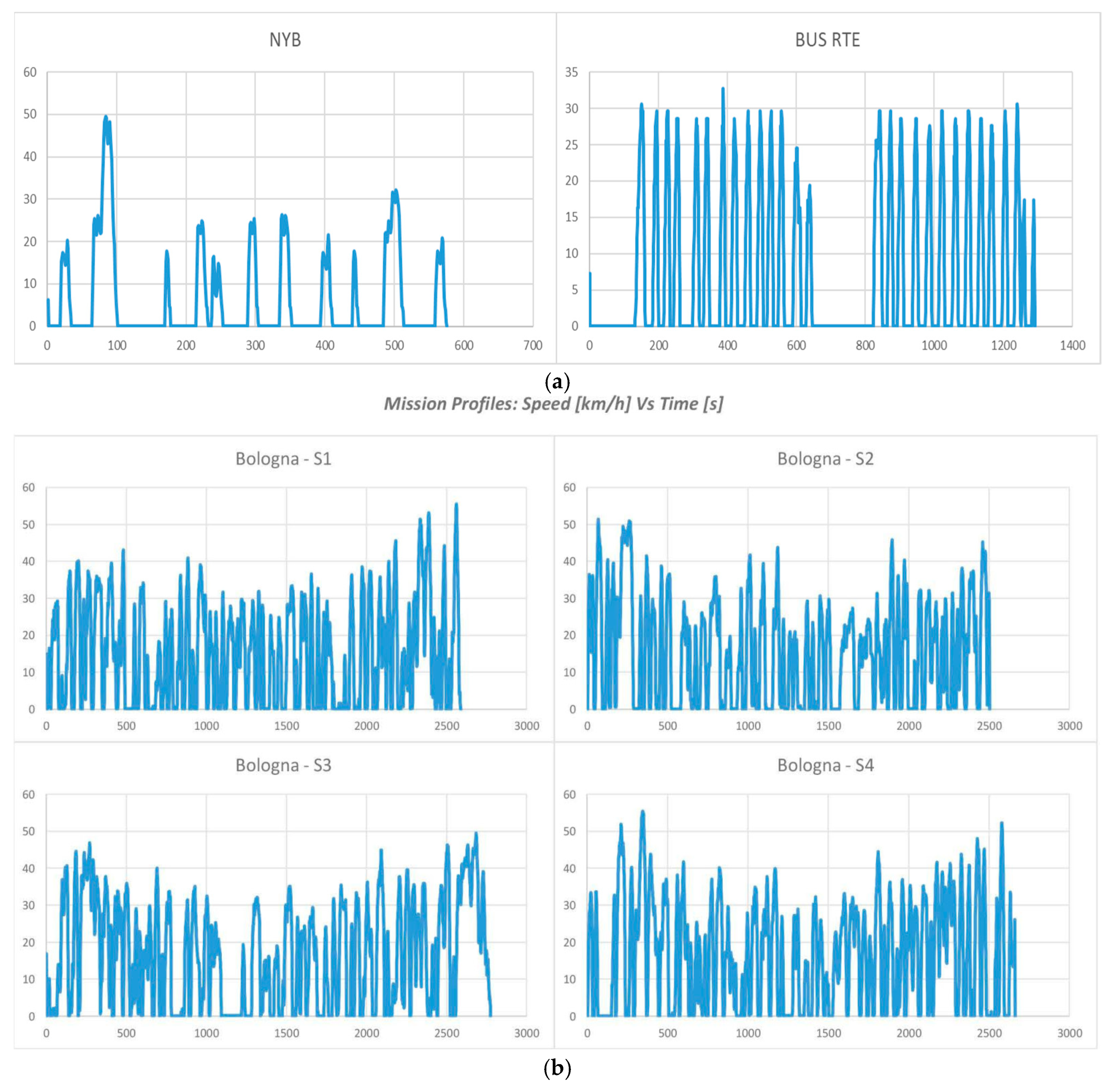
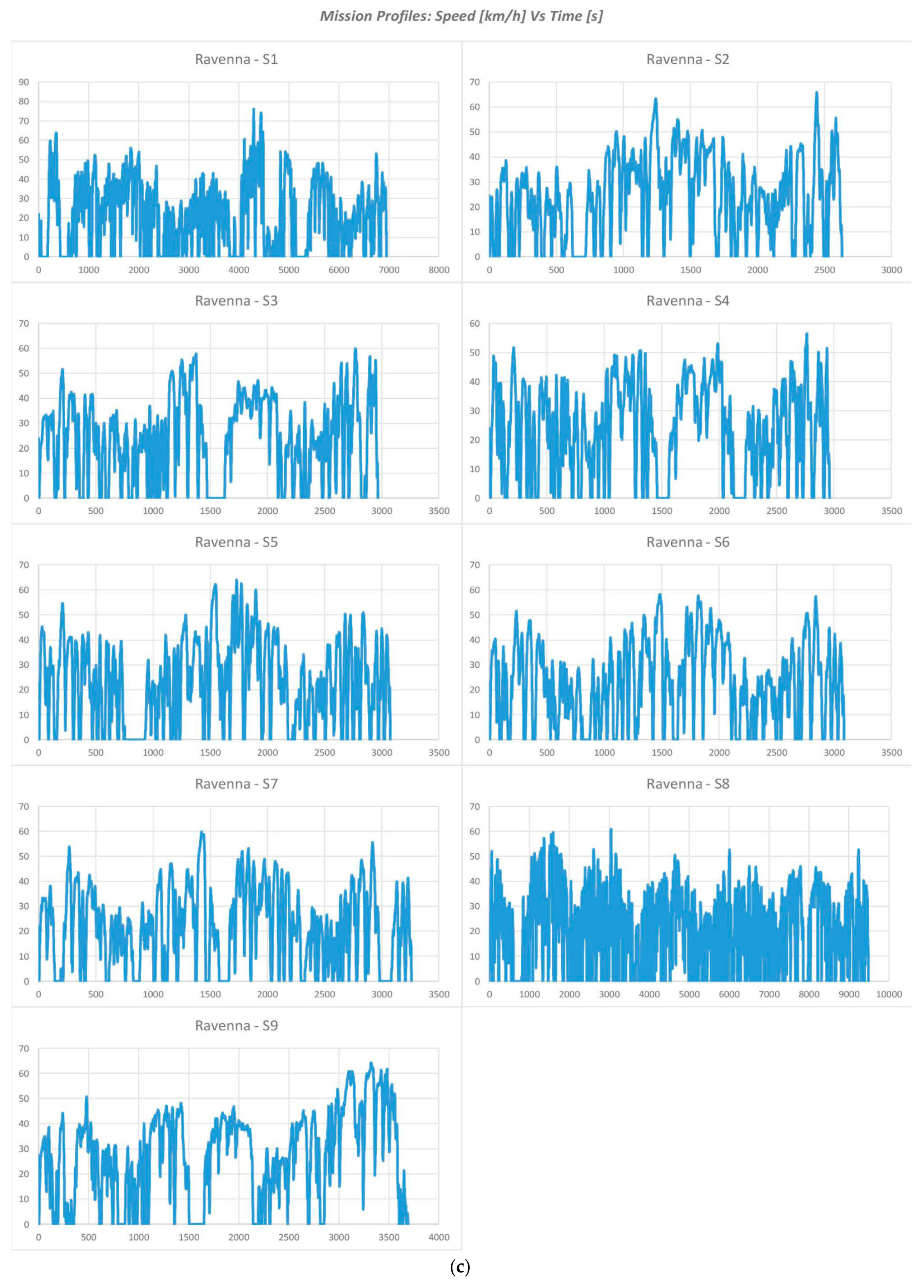
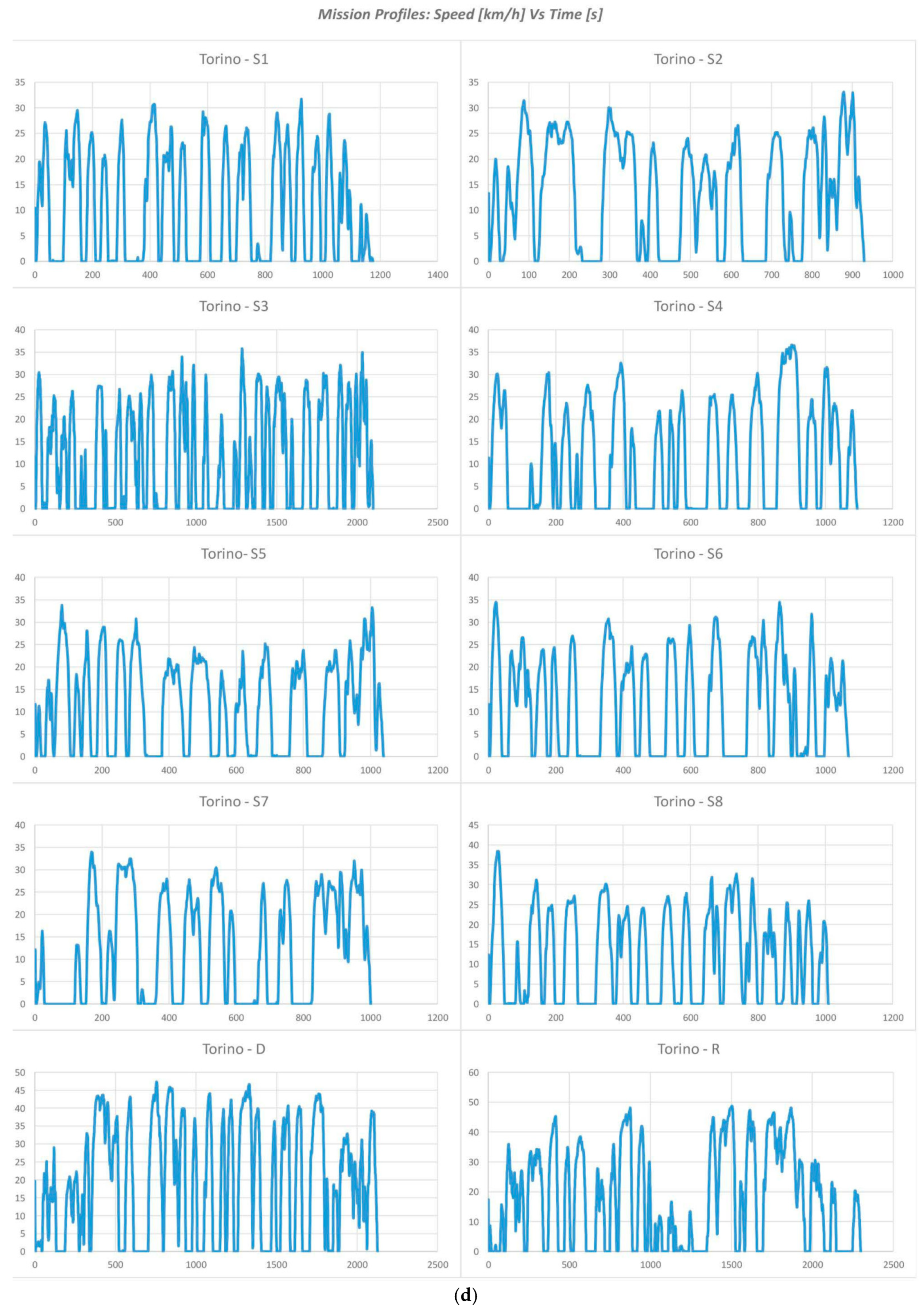
All the procedures take the lead from measurements done on real-operation buses in 23 different road and traffic conditions in Italy.

The 23 cycles were surveyed in the cities of Ravenna, Turin and Bologna and cover a commercial speed range, ranging between 10 and 27 km/h.

To widen the operating range, two international cycles with lower commercial speed were added to these: these cycles are available in the literature and were measured on buses operating in the city of New York (they are known as “NYB” and “BUSRTE” cycles). The kinematic profiles (Vehicle speed in km/h versus Cycle time in s) of the 25 cycles are shown in Figure 1.

The cycles were firstly analyzed from the kinematic point of view, identifying the average route covered between two stops (named “arc”), the average duration of stops and the percentage of stop time.

The results of this statistical analysis are reported in the central part of

Table 1. Kinematic characteristics of the measured mission profiles.

CYCLE	KINEMATIC ANALYSYS			STOPS ANALYSIS						ENERGY ANALYSIS
Name	Distance	V Mean	V Max	Mean Arc between Stops			%	Mean	Max	+	-	−/+
--	km	km/h	km/h	m	s	km/h	%	s	s	Wh/(km*t)	Wh/(km*t)	%
NYB	1.0	6.2	49.6	90	34	9.5	34	18	68	155	65	42
BUS RTE	2.6	7.2	32.7	93	34	10.0	27	13	178	138	61	44
T-S1	3.4	10.4	31.7	189	48	14.2	26	17	65	84	25	30
T-S4	3.5	11.4	36.6	192	45	15.2	25	15	65	84	23	28
T-S6	3.5	11.7	34.5	203	48	15.3	24	15	69	84	25	30
T-S5	3.4	11.7	33.8	224	54	15.1	22	15	52	77	20	26
T-S3	6.8	11.7	35.8	207	49	15.3	24	15	59	79	21	26
T-S7	3.4	12.1	34.0	258	54	17.3	30	23	91	77	19	24
T-S8	3.4	12.3	38.4	191	45	15.3	19	11	53	88	27	31
T-S2	3.4	13.3	33.1	342	70	17.5	24	12	57	74	17	24
B-S1	10.7	14.9	55.5	170	36	17.0	12	5	51	109	39	36
B-S2	10.7	15.3	51.4	214	43	18.1	15	8	60	103	35	33
B-S4	12.4	16.6	55.4	248	46	19.4	15	8	86	103	35	34
B-S3	13.0	16.8	49.5	265	49	19.5	14	8	127	91	25	28
T-R	11.1	17.4	48.7	445	64	25.1	30	28	87	83	17	21
T-D	11.4	19.6	47.3	544	73	26.7	27	237	90	88	21	24
R-S7	19.7	21.7	59.8	596	80	26.8	19	19	85	93	25	27
R-S8	58.0	22.0	60.9	906	127	25.7	14	21	205	54	15	28
R-S1	42.6	22.0	76.2	818	105	28.2	22	29	156	72	18	25
R-S6	19.7	22.9	58.2	546	74	26.6	14	12	60	94	25	27
R-S5	19.7	23.1	64.1	562	73	27.8	17	15	175	103	32	31
R-S3	19.6	23.9	60.0	634	79	28.8	17	16	154	97	27	28
R-S4	19.7	23.9	56.6	678	85	28.8	17	17	100	99	29	30
R-S2	17.8	24.4	66.0	556	72	27.6	12	10	98	98	28	28
R-S9	28.1	27.4	64.3	825	92	32.4	16	17	150	89	17	20

, in particular in the columns referred to with the definition of “Stops Analysis”.

An energy analysis was therefore carried out on the same cycles. To this end, a reference vehicle (in terms of mass and typical geometries) was imagined to cover the route. The results obtained were returned in specific terms (such as Wh spent per ton and per km traveled) to generalize the analysis.

To calculate the energies required for wind rolling and aerodynamic losses of the vehicle, standard correlations were used, widely consolidated in the literature.

Through the following equations, it is possible to calculate the energies required for traction, as well as the braking energy of the vehicle, which constitutes the theoretical energy potential that can be recovered by suitably equipped vehicles (such as electrical ones).

$$P_{Rolling}=-\left[m·g·\cos \left(\alpha \right)·\left(C_{R_0}+C_{R_1}\mathrm{v}\left(t\right)\right)\right]·\mathrm{v}\left(t\right)$$

(1)

$$P_{Aero}=-\left[\frac{1}{2}·\rho ·C_X·A·{\mathrm{v}}^2\left(t\right)\right]·\mathrm{v}\left(t\right)$$

(2)

$$P_{Climbing}=-\left[m·g·\sin \left(\alpha \right)\right]·\mathrm{v}\left(t\right)$$

(3)

$$P_{Tot}=m·\mathrm{v}\left(t\right)·\frac{d\mathrm{v}\left(t\right)}{dt}-P_{Rolling}-P_{Aero}-P_{Climbing}$$

(4)

$$E_{Tot}={{\displaystyle \int }}_0^t\left[m·v\left(t\right)\frac{dv\left(t\right)}{dt}+mg\cos \left(\alpha \right)·\left(C_{R_0}\mathrm{v}\left(t\right)+C_{R_1}{v}^2\left(t\right)\right)+\frac{\rho }{2}{C}_{X}A·v^3\left(t\right)+mg\sin \left(\alpha \right)·v\left(t\right)\right]dt$$

(5)

$$E_{+,\left(Traction\right)}={{\displaystyle \int }}_0^t{P}_{Tot}·\left(P_{Tot}\ge 0\right)·dt$$

(6)

$$E_{-,\left(Regenerable\right)}={{\displaystyle \int }}_0^t{P}_{Tot}·\left(P_{Tot}<0\right)·dt$$

(7)

The following ratio defines the percentage of recoverable energy over the total energy spent for the traction of the vehicle and is fundamental in defining the performance of the vehicles and entailing different operating performances of both conventional and innovative propulsion systems:

$$E_{-,\%}=\frac{E_{-}}{E_{+}}·100$$

(8)

The results of the energetic analysis of the 25 cycles are shown on the right side of Table 1 in the columns referred to with the definition of “Energy”, with reference to a conventional full-size bus.

For each of the quantities, a strong variability is identified with mean cruise speed: for each of the main significant properties defining the mission profiles, the proper regressive best-fitting curves more accurately approximating the average behavior of the cycles with the variation of the service speed were calculated and properly stored in the software tool in Matlab.

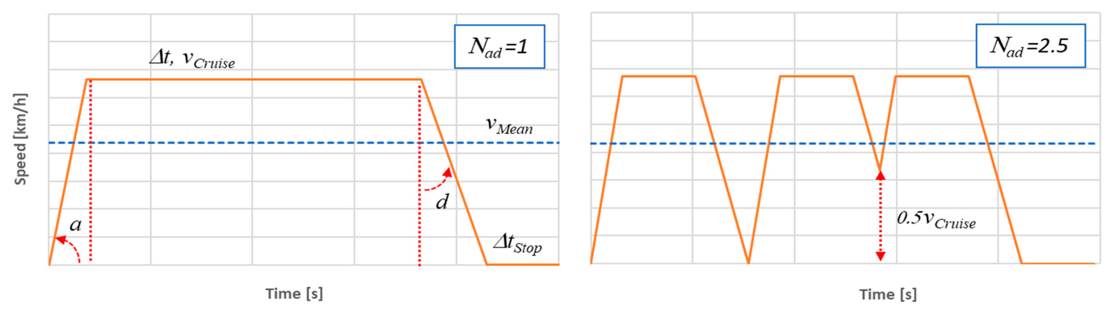
The proposed procedure may now move towards the definition of an equivalent cycle that could appropriately represent an arc of a vehicle mission for each possible given mean cruise speed, distance between the stops and time duration. The hypothesized basic cycle is an evolution of a trapezoid cycle, definable according to the scheme shown in the following figure. In practice, a complete mission given through a time schedule cycle has been reconstructed through a series of equivalent arcs in kinematic and energetic terms to the average arc detected.

To better understand the procedure, please consider Figure 2. Its left part represents a simple trapezoidal cycle, for a certain service speed, which normally has an average energy consumption that is lower than that detected experimentally for a mission characterized by the same mean cruise speed according to the previously reported data in Table 1. In the same way, braking energy percentages are usually significantly lower than in real cycles.

To make the reconstructed cycle equivalent to that foreseeable in real operations, both from a kinematic and from an energetic point of view, it is therefore necessary to add accelerations and decelerations capable of simulating, at least in overall terms, the energy characteristics of the cycle in question. To this end, a parameter has been defined, N_ad (i.e., the number of overall accelerations and decelerations in the average arc), which can also assume non-integer values. Once N_ad is fixed, the equivalent cycle can be reconstructed according to the diagram shown on the right side of Figure 2. This novel “quasi-trapezoid” cycle is a generalization version of the simple trapezoidal one, obtainable for N_ad = 1.

For the complete reconstruction of the cycle, it is now necessary to calculate all the parameters that define the complete “geometry”. Average values for the accelerations and decelerations of the vehicle during ramps can be assumed for this purpose. In particular, the deceleration can be parameterized as a fraction of the acceleration by means of a factor k_ad = d/a (fixed to 0.7 in the following calculations).

Properly integrating the motion equation in the proposed reconstructed arc of the vehicle mission (referred to in the following equations with the subscript S and G, “Stop and Go”), it is quite easy to calculate the total space traveled and the time required to travel the average arc, according to the following reports:

$$\{\begin{array}{c}{S}_{S\&G}=\frac{N_{ad}}{2·a}·\frac{k_{ad}+1}{k_{ad}}·v_{Cruise}^2+\mathrm{\Delta }{t}_{Cruise}·v_{Cruise}\\ \mathrm{\Delta }{t}_{S\&G}=\frac{N_{ad}}{a}·\frac{k_{ad}+1}{k_{ad}}·v_{Cruise}+\mathrm{\Delta }{t}_{Cruise}\end{array}$$

(9)

Then, the duration of the stop can be calculated starting from the estimate made on the percentage of stop time on the total mission time (S_%):

$$\mathrm{\Delta }{t}_{Stop}=\mathrm{\Delta }{t}_{S\&G}·\frac{{\overline{S}}_{\%}}{100-{\overline{S}}_{\%}}$$

(10)

Combining previous equations, it is now possible to calculate the required cruising speed and the time it has to be maintained within the arc, according to the following formulas:

$$\to \{\begin{array}{c}{v}_{Cruise}=\frac{-b_{II}\pm \sqrt{b_{II}^2-4a_{II}{c}_{II}}}{2a_{II}};a_{II}=\frac{N_{ad}}{2}·\left(\frac{1}{a}+\frac{1}{d}\right);b_{II}=\mathrm{\Delta }{t}_{S\&G};c_{II}=S_{S\&G}\\ \mathrm{\Delta }{t}_{Cruise}=\mathrm{\Delta }{t}_{S\&G}-\left(\frac{1}{a}+\frac{1}{d}\right)·N_{ad}·v_{Cruise}\end{array}$$

(11)

Those values are therefore still dependent on the imposed value for N_ad.

Energetic evaluation of the arc may now be performed, integrating the equations defining required power output for the reference vehicle, using well-consolidated formulations from the literature for air drag and rolling resistance. For simplicity, the formulas below were reported on a flat route hypothesis. However, the same calculation may be easily performed including energy requirements for inclined routes:

Acceleration ramp:

$$E_a=N_{ad}·\frac{m·v_{Cruise}^2}{2}\left\{1+\frac{1}{a}\left[g\left(C_{R_0}+\frac{2}{3}{C}_{R_1}{v}_{Cruise}\right)+\frac{\rho C_{X}A}{4·m}{v}_{Cruise}^2\right]\right\}$$

(12)

Cruise:

$$E_{Cruise}=v_{Cruise}\left[mg\left(C_{R_0}+C_{R_1}{v}_{Cruise}\right)+\frac{\rho }{2}·C_X·A·v_{Cruise}^2\right]·\mathrm{\Delta }{t}_{Cruise}$$

(13)

Deceleration ramp:

$$E_d=N_{ad}·\frac{m·v_{Cruise}^2}{2}·\left\{-1+\frac{1}{k_{ad}·a}\left[g\left(C_{R_0}+\frac{2}{3}{C}_{R_1}{v}_{Cruise}\right)+\frac{\rho C_{X}A}{4·m}{v}_{Cruise}^2\right]\right\}$$

(14)

The reported formulas also permit the calculation of the total traction energy and of regenerable energy within the reconstructed arc: please consider that, when the inclined route is also considered, recoverable energy is concentrated in the deceleration ramp, unless a very high positive or negative slope is considered. It is therefore possible to calculate:

Energy Traction:

$$E_{+,sp}=\frac{E_a+E_{Cruise}}{m·S_{S\&G}}$$

(15)

Regenerable energy:

$$E_{-,sp}=\frac{-E_d}{m·S_{S\&G}}$$

(16)

Regenerable fraction:

$$E_{-,\%}=\frac{E_{-,sp}}{E_{+,sp}}·100$$

(17)

It is possible to implement the proposed procedure to build a kinematically and energetically equivalent mission for a bus be involved in a programming plan set by a public transport company.

To illustrate the procedure identified with a real case, we will refer below to the programming plan for the first morning mission of the Rome bus Line #90. The main data relating to the line time schedule are shown on the left side of

Table 2. Scheduled Timetable of the “LINEA90” in Rome.

	ROME - LINE 90 SCHEDULED SERVICE		ARC		Speed	S&S	Stops			E+	E-	−/+%
	DA	A	m	s	km/h	m	%	#	s	Wh/(km/t)		-
ARC 1	LABIA	BULGARELLI	1090	231	17.0	322.8	19.9	2.0	15.3	94.5	27.4	29.0
ARC 2	BULGARELLI	VIMERCATI	1175	249	17.0	322.5	19.9	3.0	12.4	94.5	27.4	29.0
ARC 3	VIMERCATI	CERVIALTO	1025	207	17.8	357.6	19.3	2.0	13.3	92.1	26.0	28.3
ARC 4	CERVIALTO	EUGANEI	605	123	17.7	352.9	19.3	1.0	11.9	92.4	26.2	28.4
ARC 5	EUGANEI	M.TE GENNARO	638	129	17.8	356.3	19.3	1.0	12.4	92.2	26.1	28.3
ARC 6	M.TE GENNARO	STELVIO	420	85	17.8	356.0	19.3	0.0	16.4	92.2	26.1	28.3
ARC 7	STELVIO	C.SO SEMPIONE	1133	229	17.8	357.1	19.3	2.0	14.7	92.1	26.0	28.3
ARC 8	C.SO SEMPIONE	VAL D’OSSOLA	337	68	17.9	359.4	19.2	0.0	13.1	92.0	26.0	28.2
ARC 9	VAL D’OSSOLA	VAL D’AOSTA	400	81	17.8	356.1	19.3	0.0	15.6	92.2	26.1	28.3
ARC 10	VAL D’AOSTA	BATTERIA	421	86	17.6	348.9	19.4	0.0	16.7	92.7	26.4	28.4
ARC 11	BATTERIA	ASMARA	334	67	17.9	362.4	19.2	0.0	12.8	91.8	25.8	28.2
ARC 12	ASMARA	XXI APRILE	694	141	17.7	352.5	19.4	1.0	13.6	92.4	26.2	28.4
ARC 13	XXI APRILE	MARGHERITA	1177	238	17.8	356.6	19.3	2.0	15.3	92.1	26.1	28.3
ARC 14	MARGHERITA	PORTA PIA	545	110	17.8	358.7	19.2	1.0	10.6	92.0	26.0	28.2
ARC 15	PORTA PIA	XX SETTEMBRE	671	136	17.7	354.3	19.3	1.0	13.1	92.3	26.1	28.3
ARC 16	XX SETTEMBRE	TERMINI	1089	220	17.8	357.4	19.3	2.0	14.1	92.1	26.0	28.3

.

The data obtainable from the time-schedule allow (through the geo-referencing of the stops) the calculation of the length of the 16 arcs of the path identifiable between the individual stops and the time in which they are served (including the stop time at the stop served at the end of the arc). As already done previously, for simplicity, the effects of the average slopes along the single middle arcs are not included in the analysis. The procedure can, however, be very simply generalized to include the average energy effects of the possible slope of the path along the arcs.

The reconstruction of the vehicle’s mission now takes place by repeating what has been done previously for each of the mean arcs identified and therefore, separately reconstructing 16 cycle sections, corresponding to the 16 arcs of the complete scheduled mission. Each of these 16 sections of the overall cycles will be constructed as a succession of a proper number of “quasi-trapezoid” cycles representing the Start and Stops of the vehicle that will likely occur in the real mission (according to mean experimental data at a certain mean cruise speed, also representing traffic conditions, crossings, light, etc.).

Here, in fact, we must distinguish between service stops (notes) and those due to congestion and/or traffic lights, crossings and other events. We cannot have knowledge of these additional stops from the schedule timetable, but they must be inserted artificially in a suitable manner. To this end, it is possible to proceed on a statistical basis using the data collected on the 25 basic missions analyzed, which allowed us, as already described, albeit approximately, to identify the variability of the average arc length between two stops (for whatever reason they are to be attributed) to the variation of the average speed foreseen for the service ((indicated below as S_S&G(v_Mean,Arc)). To this aim, v_Mean,Arc can be easily calculated from the time schedule data and is reported in the right part of Table 1. In the same table, all the other kinematic and energetic parameters expected for the arc to be performed during real vehicle operation at that given cruise speed are reported: those were according to the best-fitting curves reported and detailed in Table 2.

Once S_S&G(v_Mean,Arc) has been estimated, the number of additional stops to be included within each arc may be imposed as:

$$N_{S\&G}=int\left(\frac{S_{Arc}}{{\overline{S}}_{S\&G}\left(v_{Mean,Arc}\right)}\right)$$

(18)

At this point, the average arc between two service stops can be effectively reconstructed by means of a proper integer N_S&G of “quasi-trapezoid” missions, each of which have a duration and length that can be calculated based on the given time-schedule through the following relations:

$$\{\begin{array}{c}\mathrm{\Delta }{t}_{S\&G,tot}=\frac{t_{Arc}}{N_{S\&G}}\\ S_{S\&G}=\frac{S_{Arc}}{N_{S\&G}}\end{array}$$

(19)

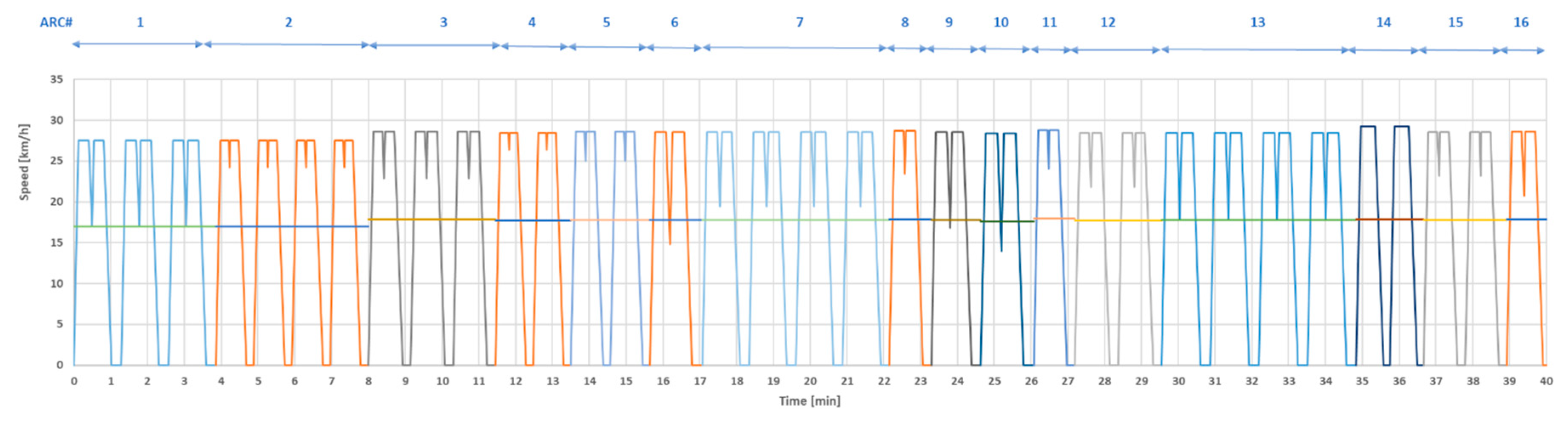
Proceeding iteratively in the same way for the sixteen mission arcs, sixteen “quasi-trapezoid” energy-equivalent arc mission profiles can be reconstructed. The succession of the 16 arches will therefore represent the overall mission equivalent to the cinematic- and energetic-equivalent to the service to be performed based on the programming plan set for Line 90 of Rome (specifically for the first morning service of the vehicle). The resulting mission is represented in Figure 3. Figure 3 also reports the mean cruise speeds of each one of the 16 mission arcs.

According to this approach, a SW tool has been realized in a Matlab environment by the author, able to reconstruct any possible mission based on the time schedule of a vehicle, given by the geographic position of the stops and their service times, also considering the effect of the mean inclination of the road between the stops.

3. Conclusions

The present paper takes the lead from the long-lasting experience gained by the author on mathematical modeling of vehicle energy performances and on the calibration of those models based on real data acquired on buses in real operation.

The procedure for the derivation of the proposed schedule-based energy-equivalent driving cycle for buses was explained in detail. Specific attention was given to the energy-equivalency of the proposed driving cycles to the foreseeable real mission of the vehicles on their scheduled duty (e.g., mean inertial energy on play during vehicle Start and Stops, mean stops in between the arcs, mean vehicle speed and acceleration, etc.): the objective was in fact that of reproducing the same energy characteristics of the real vehicle mission in a simplified way. To this aim, the main energy characteristics of the expected mission were foreseen through a regressive interpolation of data coming from an extensive analysis of onboard measured data, based on independent variables (mean vehicle cruise speed and slope), which could be efficiently estimated by vehicle schedule.

The procedure is in fact based on the automatic reconstruction of the mission through a series of properly sized “quasi-trapezoid” missions, whose main kinematic parameters may be adjusted based on the simple knowledge of mean vehicle cruise speed.

A SW tool implementing this procedure has also been realized in a Matlab environment by the author, and is able to automatically reconstruct any possible mission based on the time schedule of a vehicle, given by the geographic position of the stops and their service times, also considering the effect of the mean inclination of the road between the stops.

The energy equivalency of the reconstructed driving cycle to the foreseeable real-time vehicle mission makes any possible optimization activity on the vehicle (both in its design phase and in its real-time operation) much more reliable than in usual practice (which normally makes reference to standardized bus cycles with very limited connection to expected vehicle use).

There could be a number of possible uses of the so-defined driving cycles (e.g., for buses’ performance prediction, propulsion systems choice and net optimization).